Mapping Precipitation, Temperature, and Evapotranspiration in the Mkomazi River Basin, Tanzania

Abstract

It is still a challenge to provide spatially explicit predictions of climate parameters in African regions of complex relief, where meteorological information is scarce. Here we predict rainfall, temperature, and reference evapotranspiration (ET_o) for the southern Mkomazi River Basin in Northeastern Tanzania, East Africa, by means of regression-based, digital elevation models (DEM) at 90 m spatial-resolution and geographic information systems (GIS) techniques. We mapped rainfall for the period 1964–2010. The models accounted for orographic factors which strongly influenced the spatial variability of rainfall in the region. According to orography, the area was divided into three zones for modelling rainfall: windward, leeward, and transition zone. Rainfall indicates high spatial and temporal variability dominated by equatorial East-African climate circulation systems. Maximum and minimum temperatures were modelled for the period 1989–1994, the models accounted only for the altitude gradient. Mean temperature was calculated by arithmetic mean of maximum and minimum temperatures maps in ArcGIS. ET_o was estimated in ArcGIS following the method described by Hargreaves and Samani. The maps were made on a monthly basis for rainfall, ET_o, and mean, maximum, and minimum temperatures. The obtained maps are useful for the purpose of agriculture, ecological, and water resources management.

1. Introduction

Accurate precipitation, temperature, and evapotranspiration maps at landscape scales are needed for many applications in agriculture, climate forecasting, irrigation schemes, and water provisioning. These climatic maps are important in ecological studies because precipitation, temperature, and evapotranspiration strongly influence the transfer of moisture between the surface and the atmosphere at local and regional levels. Precipitation is the main source of water in the terrestrial water cycle, while evapotranspiration returns about 65% of precipitation into the atmosphere, depending on the vegetation cover [1]. The sun as a black body emits energy at 5530 °C, averaged over the year, and of all surfaces of the earth this amounts to 342 W m⁻². Some amount of the solar energy is used for all plant physiological processes and sets up large-scale climatic conditions and patterns.

Precipitation and temperature are mostly measured at meteorological stations. Evapotranspiration is commonly assessed indirectly by either (i) considering the energy balance at land surface [2]; (ii) by measuring eddy covariance at some distance above the land surface [3]; (iii) by a water balance approach for watersheds when precipitation, change in storage, and stream discharge are known [2]; or (iv) by estimating reference evapotranspiration (ET_o) from a hypothetical surface of green grass cover of uniform height of 0.12 m adequately watered with surface resistance of 70 s m⁻¹ and albedo of 0.23 [4].

Precipitation and temperature patterns on the earth’s surface are determined by the combination of geographic factors such as altitude, latitude, aspect and exposure, atmospheric circulations, characteristics of ocean currents, and effects of continentality [5]. Mountain climates are controlled by the same factors, with their hydrological and ecological systems being sensitive to climate variability [6], confounded by local variety of combinations created by orientation, spacing, and steepness of slopes, along with the presence of complex patterns of snow patches, shade, vegetation, and soil. By acting as a barrier, mountains themselves affect local and regional climates and modify passing storms. When mountain ranges are oriented perpendicular to the prevailing winds, forced ascent of air is usually most effective; the more exposed the slope, the more rapidly air will be forced to rise and cool, which results in precipitation. Great variations in precipitation and temperature occur over relatively short distances; one slope may be excessively wet with more precipitation at higher elevations, while another is relatively dry [7].

Different interpolation or extrapolation methods can be conceived to map climate variables in a spatially explicit way. Over the last few decades, geostatistic interpolation methods [8] became commonly used and recognized to have several advantages [9] over non-geostatistic methods such as Thiessen polygon, inverse distance weighting, or isohyetal methods.

Many research studies have used geostatistic techniques which consider topographic variations in mapping climatological variables on mountains terrain. Studies exemplifying these approaches are [10] for precipitation and [11] for evapotranspiration. However, most of these interpolation techniques do not take into account the effect of relief and other geographic factors. For that reason, interpolation techniques should take into account the potential effects of topographical factors on the spatial distribution of climatic variables. Such interpolation techniques (universal techniques) use geographic information systems (GIS) and digital elevation models (DEMs) for spatial analyses [12].

Several researchers have demonstrated the potential of universal techniques on mapping precipitation [13], temperature [14], and evapotranspiration [15]. In these regression-based techniques, geographic and topographic factors that control the spatial distribution of climate are used as independent variables [16], and dependence models are created between the climate data and independent variables. The main advantage of this technique is that maps are compiled from weather stations and auxiliary information that describe geographic and topographic variables which improves the accuracy and spatial detail of the maps. A goal of the present study is to apply universal interpolation methods and GIS technologies in mapping precipitation, temperature, and evapotranspiration of the southern Mkomazi River Basin, an East-African mountainous region including parts of the Pare and Usambara mountains. The region is typical for remote East-African rural areas, where most of the population settles on the slopes of the mountains and in the vicinity of the river, whereas the semi-arid plains are scarcely populated.

The climate of the southern Mkomazi River Basin is characterized by two distinct rainfall seasons. Long-rains in March–May are commonly abundant [17], whereas short-rains in October–December reveal more interannual variability [18]. This bimodal pattern is largely related to the seasonal migration of the inter-tropical convergence zone (ITCZ) across the equator [19].

There are two essential phenomena influencing the interannual rainfall variability in this region: (i) the El Niño-Southern Oscillation (ENSO) [20]; and (ii) the Indian Ocean dipole (IOD) [21] or Indian Ocean zonal model (IOZM) [22]. Both extreme weather events can bring large floods [23] or strong droughts [24], which severely affect the livelihoods of the people.

Therefore, better knowledge of the spatial distribution of precipitation, temperature, and evapotranspiration is required, particularly in areas with strong variations in topography and elevation [13,15]. To address this, the present study uses regression-based techniques and GIS knowledge to construct monthly maps of precipitation, temperature, and evapotranspiration, accounting for major topographic influences, particularly elevation, surface orientation, and obstruction by surrounding topographic features.

Unfortunately, the number of meteorological stations where precipitation, air temperature, wind speed, humidity, and solar radiation are observed is limited in many parts of the globe, particularly in developing countries. Many sub-Saharan countries continue to experience difficulties with the availability of long-term climatic data, and available information is sparse with numerous prolonged gaps both in time and space. These limitations in the quantity and quality of site observations impose substantial constraints on studies of the climatic variability, particularly in the southern Mkomazi River Basin in Tanzania. Therefore, our study involved additional efforts of data correction and dealing with missing data.

2. Materials and Methods

2.1. Study Area

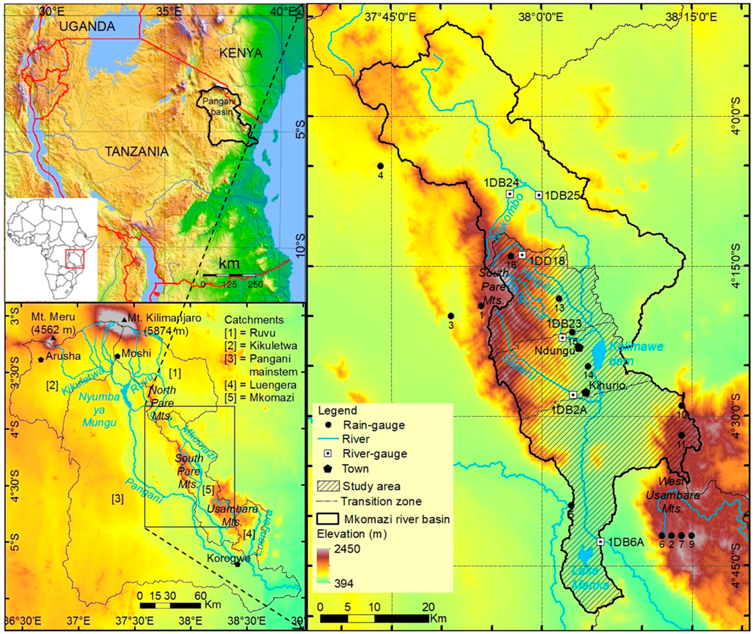
The southern Mkomazi River Basin, located at latitude (4°10′ S–4°50′ S) and longitude (37°50′ E–38°20′ E) with a size of approximately 1188 km² (Figure 1), is the mountainous sub-catchment in the mid-reaches of the Pangani River Basin in Northern Tanzania. The elevation above sea level ranges from 400 m along the Mkomazi valley to 2300 m and 2450 m in the West Usambara and South Pare mountains. Both mountains are covered with tropical rainforests exhibiting a high diversity of species [25]. Physiography varies from plains along the valley to rugged escarpments and steep slopes formed by erosion in the surrounding mountainous range. Livelihoods of the people depend directly or indirectly on agriculture and forest resources [26].

2.2. Data Source and Data Cleaning

We used two climatic datasets: (i) monthly rainfall averages from 23 stations provided by the Tanzania Meteorological Agency (TMA) (hereafter dataset1); and (ii) Pangani-NRM-version-2.0 (hereafter dataset2) daily rainfall and temperature records. Dataset2 consolidates climatological records collected from the Tanzania Ministry of Water and Livestock Development, TMA, Pangani River Basin district, and regional offices and institutions.

For rainfall, the two datasets of most but not all stations show similar characteristics in terms of record lengths, monthly averages sums and missing data. We used datset1 for our analysis since most of its record lengths spanned to recent years and used dataset2 to fill gaps in dataset1. With this procedure, we were able to replace 10% of the missing rainfall data.

Both systematic and random errors exist in station data [27]. Errors can be caused by wind, wetting, and evaporation losses, and type and location of the weather gauge station [28]. In addition, there are human associated errors like misread and mistyped records [29]. Such erroneous station data have been identified as inhomogeneous data or outliers [30]. Quality control of climatological data constitutes a key point in climate research [31], and it depends on the quality of the reference series [32], in which high correlation and vicinity is a general agreement on how to select neighbor stations for reference series [33]. Some examples of statistical methods for identifying outliers include the biweight mean and standard deviation method [34], and the traditional methods based on the mean and standard deviation.

In the present study, all rainfall stations were selected for constructing reference series. A traditional statistical method was used to identify outliers: estimate the mean and standard deviation, and transform the original values through standardization into “Z-scores”, then discard all values greater than a predefined limit. We used such a method for each calendar month of each year separately based on the premise that an individual station’s value should be similar in a statistical sense. Knowing that there is a sample size dependent on the largest Z-score that can occur in a finite sample [35], we predefined a standard deviation limit of greater than 50% Z-score to pass for outliers.

Very few stations in dataset1 had complete records from the 1930s to recent years. Therefore, our analysis concentrated on the period 1964–2010, as it comprised 75% of all rainfall records of dataset1. Temperature was analyzed for the period 1989–1994 because of limited availability of temperature records in higher altitudes. Note that we aimed to establish a relationship between climate variables and altitude. Seven stations, of records end-date before 1964, and of less than 30% of available records relative to the period 1964–2010, were not included into the dataset for analysis of rainfall. The dataset (at month scale) included sixteen rainfall and three temperature stations (

Table 1. Rainfall and temperature gauge network. Temperature stations are marked *, whereas superscripts ‘^w’, ‘^l’ and ‘^r’ indicate windward, leeward, and ridge rainfall stations, respectively. Missing data are described relatively to start-end-date for each gauge station, and values in parentheses are relatively to the period 1964–2010 for rainfall and 1989–1994 for temperature.

Station Number	Gauge Name	Gauge ID	Elevation (m a.s.l.)	Latitude	Longitude	Record Length	Missing (%)
1	Suji Mission l	9437004	1371	−4.317	37.850	1923−2008	18 (32)
2	Mazinde Factory l	9438019	1996	−4.700	38.217	1929−2010	6 (7)
3	Hassan Sisal Estate l	9437001	914	−4.333	37.850	1933−2007	21 (29)
4	Same Met l	9437003	860	−4.083	37.733	1934−2011	1 (0)
5	Buiko Hydromet l	9438009	534	−4.650	38.050	1962−2005	1 (11)
6	Shume Forest l	9438012	1889	−4.700	38.200	1937−1997	5 (6)
7	Gologolo Forest House l	9438047	1920	−4.700	38.233	1964−2009	41 (41)
8	Gologolo l	9438037	1882	−4.700	38.233	1955−1986	7 (56)
9	Mlomboza r	9438046	2286	−4.700	38.250	1964−1997	1 (29)
10	Mtae Pr Court l	9438066	1559	−4.483	38.233	1971−2010	22 (22)
11	Shagavu Forest Nursery l	9438049	1981	−4.533	38.233	1964−2011	6 (6)
12	Shagavu l	9438034	1828	−4.533	38.217	1955−2011	5 (3)
13	Gonja Estate w	9438011	584	−4.300	38.033	1937−1988	10 (50)
14	Kalimawe w	9438040	488	−4.417	38.083	1963−2010	40 (41)
15	Ndungu Sisal Estate w	9438051	533	−4.367	38.050	1966−2002	16 (34)
16	Tia Dam w	9437010	1676	−4.233	37.950	1962−2010	32 (31)
101	* Lushoto Hydromet	9438076	1631	−4.783	38.267	1989−1994	1 (1)
102	* Moshi Airport	9337004	854	−3.350	37.333	1958−1993	2 (18)
103	* Same Met	9437003	860	−4.083	37.733	1958−2010	8 (2)

). We used mean values (MVs) and standard deviations (SDs) to describe rainfall, and maximum and minimum temperatures temporal variability.

Station elevations ranged from 488 m for station 14 in the Mkomazi valley to 2286 m for station 9 in the West Usambara mountains. Gauge altitude was corrected using a DEM at 90 m (www2.jpl.nasa.gov/srtm/) spatial-resolution for discrepancy greater than 500 m for stations 2 and 10. The dataset was cleaned for outliers, such as too high rainfall in February (1965 for station 1, 1984 and 1985 for station 9), May 1975 for station 8, June (1966, 1969, 1971) for station 3, and zero values during the entire year 1994 for station 9. Daily rainfall records were aggregated to monthly values for station 5, and missing data for station 16 were filled by accumulated daily records. The dataset included eight rainfall stations within the study area boundary, thus the network density was 74 km² gauge⁻¹ when all rainfall stations in the dataset counted.

Unlike for rainfall data quality control and outlier’s limit rejection, monthly maximum and minimum temperatures were compared only to ensure that the latter do not exceed the former, as temperature possesses less spatial-temporal variability than does rainfall [33]. Missing data for maximum and minimum temperatures (T_i,j), in which maximum temperature in February 1992 were filled for station 101, was calculated as

$${\mathrm{T}}_{\mathrm{i},\mathrm{j}}=0.5\left({\mathrm{T}}_{\mathrm{i},\mathrm{j}-1}+{\mathrm{T}}_{\mathrm{i},\mathrm{j}+1}\right)$$

(1)

where T_i,j−1 and T_i,j+1 are temperature (°C) data followed and preceded by the missing data, and j is the month of year i.

2.3. Spatial Interpolation of Rainfall

The precipitation–elevation relationships on mountains can vary noticeably from terrain to terrain, and are influenced by factors such as steepness and orientation of the terrain, and upward wind effects, among others. Rainfall stations were divided into three groups according to orographic barriers: (i) stations on the eastern slopes of South Pare mountains (windward side); (ii) stations on the western slopes of West Usambara mountains (leeward side); and (iii) stations located at the ridge. Grouped stations resulted in strengthening precipitation–elevation relationships [13].

To effectively predict the spatial pattern of orographic precipitation in complex terrain, the model should include physical elements such as airflow dynamics in both vertical and horizontal scales [36,37]. However, relatively high data demands limit the use of airflow dynamics in most areas of data scarcity like in the Mkomazi River Basin. Therefore, to predict the spatial pattern of rainfall, we considered only altitude and aspect correction, and assumed that condensed water falls immediately to the ground.

The landscape was divided into three topographic zones which reflect different orographic precipitation regimes: windward, leeward, and transition zones. We used ArcGIS to hypothetically determine the surface illumination and the shadow surface of the West Usambara mountains. According to our field observations and the vegetation pattern, the transition zone (local variability of rainfall distribution) is between the towns of Ndungu and Kihurio (see Figure 1 for the location), and increasing northward of the former while decreasing southward of the latter. The shadow surface contours attained the best fit line between Ndungu and Kihurio towns, and the transition zone was obtained as a buffered zone around the line.

Local increases in rainfall with elevation often approximate a linear or curved distribution [38] in many regions. Under some conditions climate variables can best be estimated by non-linear regression models [39]. However, the linear form is easy to use where there are precipitation–elevation relationships and appears to be an acceptable approximation in most situations [13].

We modelled windward and leeward zones by means of linear regression-based interpolation, and constructed rainfall maps using DEM at 90 m (www2.jpl.nasa.gov/srtm/) spatial resolution in ArcGIS. Monthly precipitation, P_{i, j} (mm), for windward and leeward zones was calculated as

$${\mathrm{P}}_{\mathrm{i},\mathrm{j}}={\mathrm{b}}_0+{\mathrm{b}}_1{\mathrm{E}}_{\mathrm{i},\mathrm{j}}$$

(2)

where b₁ and b₀ are respectively, the monthly regression slopes (mm m⁻¹) and intercepts, E_i,j is the DEM elevation above sea level (m), and i is latitude of longitude j. We performed a leave-one-out test to assess the sensitivity of the model goodness-of-fit to the number of stations included in the dataset. Monthly rainfall maps for the transition zone were modelled by means of layer algebra in ArcGIS as a function of the constructed windward and leeward monthly rainfall maps, latitude, and longitude. Thus, the transition zone rainfall maps, Pt_{i, j} (mm), were calculated as

$${\mathrm{Pt}}_{\mathrm{i},\mathrm{j}}={\mathrm{b}}_{0\mathrm{s}}+\left({\mathrm{b}}_{\mathrm{on}}-{\mathrm{b}}_{0\mathrm{s}}\right)\mathsf{\omega }+\left({\mathrm{b}}_{1\mathrm{s}}+\left({\mathrm{b}}_{1\mathrm{n}}-{\mathrm{b}}_{1\mathrm{s}}\right)\mathsf{\omega }\right){\mathrm{E}}_{\mathrm{i},\mathrm{j}}$$

(3)

where b_1n and b_1s are monthly regression slopes (mm m⁻¹) for windward and leeward zones, b_0n and b_0s are regression intercepts, and ω is the distance weighting between windward or leeward and transition zone at latitude i of longitude j.

2.4. Spatial Interpolation of Temperature and Evapotranspiration

Several methods such as Blaney–Criddle, Hargreaves and Samani, Penman–Monteith, Priestly–Taylor and Thornthwaite were developed to calculate reference evapotranspiration (ET_o). The Food and Agriculture Organization of the United Nations (FAO-56) [4] has recommended Penman–Monteith as the standard method for computing ET_o from climate data. The Penman–Monteith model, which incorporates thermodynamic and aerodynamic aspects, has proved to be a relatively accurate method in both humid and arid climates. However, a relatively high data demand is a major drawback to the application of Penman–Monteith. In addition to air temperature available at most meteorological stations, Penman–Monteith requires measurements of wind speed, humidity, and solar radiation, which are observed at relatively few African weather stations.

In locations like Mkomazi River Basin, where only maximum and minimum temperatures are available, it is impractical to use the Penman–Monteith. Instead, methods considering only temperature appeared feasible. Hargreaves and Samani (HS) [40] developed an empirical method using only air temperature (mean, maximum, and minimum) and extraterrestrial radiation. The latter can be calculated for a certain latitude and day of a year. Various studies showed that HS ranked best among methods that require air temperature data only [41]. The HS method is defined as

$${\mathrm{ET}}_{\mathrm{o}}=0.0023\ast 0.408{\mathrm{R}}_{\mathrm{a}}\left({\mathrm{T}}_{\mathrm{mean}}+17.8\right)\sqrt{{\mathrm{T}}_{\max }-{\mathrm{T}}_{\min }}$$

(4)

where ET_o is the monthly averaged reference evapotranspiration (mm day⁻¹), R_a is the extraterrestrial radiation (MJ m⁻² day⁻¹), T_mean is averaged monthly temperature (°C), and T_max (T_min) are maximum (minimum) monthly temperature (°C). To obtain monthly evapotranspiration, ET_o must be multiplied by the number of days in the month.

Monthly maximum and minimum temperatures were modelled by means of regression-based interpolation and from DEM at 90 m spatial-resolution in ArcGIS to obtain continuous temperature maps, respectively. Such temperatures, T (°C) were calculated as

$$\mathrm{T}={\mathrm{b}}_0+{\mathrm{b}}_1{\mathrm{E}}_{\mathrm{i},\mathrm{j}}$$

(5)

where b₁ and b₀ are respectively, the monthly regression slopes (°C m⁻¹) and intercepts, E_i,j is the DEM elevation above sea level (m), and i is latitude of longitude j. Monthly mean temperature, T_mean (°C), was then calculated by arithmetic mean of maximum and minimum temperature as

$${\mathrm{T}}_{\mathrm{mean}}=0.5\left({\mathrm{T}}_{\max }+{\mathrm{T}}_{\min }\right)$$

(6)

Global solar radiation (R_s) was modelled in ArcGIS using DEM at 90 m spatial-resolution following the hemispherical upward-viewshed algorithm developed by Reference [42], in which such radiation is calculated as the sum of direct sun map and diffuse sky map solar radiations. Direct sun and diffuse sky map solar radiations were measured for each feature on the topographic surface on a monthly basis, assuming a clear sky for diffuse proportion and transmittivity. Extraterrestrial radiation (R_a) was then calculated as

$${\mathrm{R}}_{\mathrm{a}}={\mathrm{R}}_{\mathrm{s}}/\left({\mathrm{a}}_{\mathrm{s}}+{\mathrm{b}}_{\mathrm{s}}\frac{\mathrm{n}}{\mathrm{N}}\right)$$

(7)

where a_s and b_s are fractions of extraterrestrial radiation reaching the Earth. These Angstrom values vary depending on atmospheric conditions (e.g., humidity) and solar declination such as latitude and month. However, when no calibration has been carried out, the values a_s = 0.25 and b_s = 0.50 are recommended [4]. Also, the assumption n = N is recommended [4] where no number of sunshine hour n of possible maximum N are available. The HS equation was then applied in ArcGIS to construct continuous monthly ET_o maps.

We used two statistical estimators to determine performance of the constructed models for rainfall and maximum and minimum temperatures, the coefficient of determination (R²) [43], and the probability of F distribution [44].

3. Results

3.1. Dataset

The mean values of monthly rainfall ranged from 1 mm (July) for station 15 (533 m a.s.l.) along the Mkomazi valley to 250 mm (December) for station 16 (1676 m a.s.l.) in the South Pare mountains (

Table 2. Statistical descriptions of gauge stations. Station number: see Table 1. MV is mean value and SD is standard deviation. Wet and dry months colored light blue and orange, respectively.

	January	February	March	April	May	June	July	August	September	October	November	December	Annual Average
	MV ± SD	MV ± SD	MV ± SD	MV ± SD	MV ± SD	MV ± SD	MV ± SD	MV ± SD	MV ± SD	MV ± SD	MV ± SD	MV ± SD	MV ± SD
Station Number	Rainfall (mm)
1	92 ± 71	72 ± 53	142 ± 97	120 ± 61	52 ± 35	12 ± 14	5 ± 7	8 ± 11	10 ± 15	31 ± 40	129 ± 105	165 ± 89	838 ± 50
2	55 ± 58	57 ± 46	82 ± 62	142 ± 69	131 ± 77	31 ± 31	16 ± 21	15 ± 19	13 ± 29	41 ± 57	66 ± 46	75 ± 50	724 ± 47
3	60 ± 50	43 ± 35	87 ± 79	71 ± 45	40 ± 28	7 ± 17	5 ± 10	5 ± 15	8 ± 15	23 ± 29	63 ± 62	81 ± 59	493 ± 37
4	54 ± 53	43 ± 41	91 ± 89	107 ± 62	64 ± 52	12 ± 17	4 ± 7	10 ± 15	13 ± 22	39 ± 43	62 ± 62	63 ± 51	562 ± 43
5	42 ± 46	34 ± 32	59 ± 55	71 ± 46	46 ± 38	10 ± 13	7 ± 14	6 ± 10	4 ± 10	27 ± 34	32 ± 41	45 ± 56	383 ± 33
6	74 ± 60	56 ± 37	129 ± 83	149 ± 71	72 ± 40	14 ± 16	8 ± 17	5 ± 7	10 ± 18	37 ± 36	91 ± 59	95 ± 57	740 ± 42
7	64 ± 47	53 ± 39	101 ± 67	115 ± 59	67 ± 37	17 ± 16	12 ± 25	8 ± 19	13 ± 29	38 ± 34	85 ± 58	76 ± 56	649 ± 41
8	89 ± 80	75 ± 62	134 ± 91	170 ± 91	90 ± 59	22 ± 26	13 ± 26	11 ± 19	15 ± 33	50 ± 31	116 ± 53	102 ± 54	887 ± 52
9	86 ± 71	83 ± 51	141 ± 92	172 ± 70	142 ± 113	41 ± 41	20 ± 30	14 ± 23	15 ± 23	54 ± 58	113 ± 102	129 ± 90	1010 ± 64
10	47 ± 41	43 ± 36	75 ± 67	144 ± 61	92 ± 58	13 ± 13	9 ± 10	12 ± 14	15 ± 24	51 ± 46	100 ± 57	147 ± 101	748 ± 44
11	83 ± 58	61 ± 45	120 ± 72	140 ± 56	55 ± 36	7 ± 9	4 ± 5	5 ± 7	9 ± 13	52 ± 51	127 ± 71	167 ± 93	830 ± 43
12	102 ± 81	75 ± 55	132 ± 68	150 ± 51	61 ± 39	7 ± 10	4 ± 6	7 ± 9	9 ± 14	53 ± 51	140 ± 71	186 ± 108	926 ± 47
13	107 ± 67	84 ± 77	141 ± 124	118 ± 95	44 ± 36	8 ± 13	4 ± 8	9 ± 12	18 ± 24	39 ± 36	148 ± 82	229 ± 128	949 ± 59
14	47 ± 51	40 ± 36	63 ± 56	70 ± 51	25 ± 21	4 ± 5	2 ± 3	5 ± 6	13 ± 36	21 ± 15	38 ± 36	61 ± 45	389 ± 30
15	74 ± 84	62 ± 57	93 ± 98	86 ± 67	32 ± 31	3 ± 8	1 ± 4	3 ± 6	11 ± 20	28 ± 31	85 ± 77	127 ± 93	605 ± 48
16	117 ± 127	81 ± 75	153 ± 96	172 ± 70	62 ± 50	11 ± 16	5 ± 6	13 ± 16	22 ± 29	69 ± 59	244 ± 172	251 ± 162	1200 ± 73
	Maximum Temperature (°C)
101	28.1 ± 1.0	28.5 ± 0.8	27.6 ± 0.9	25.4 ± 0.4	23.2 ± 0.7	21.9 ± 0.6	21.4 ± 0.4	21.9 ± 0.4	23.9 ± 0.3	26.0 ± 0.6	26.6 ± 0.4	27.0 ± 0.4
102	31.3 ± 1.4	32.8 ± 1.2	32.2 ± 1.8	29.7 ± 1.3	27.3 ± 1.1	26.0 ± 0.4	25.5 ± 0.3	26.0 ± 0.5	28.5 ± 0.4	30.8 ± 0.5	31.9 ± 0.7	31.1 ± 0.8
103	30.9 ± 1.6	32.4 ± 1.2	31.7 ± 1.5	29.1 ± 1.0	26.7 ± 1.0	26.2 ± 0.5	25.8 ± 0.3	26.1 ± 0.6	28.2 ± 0.4	30.2 ± 0.5	30.7 ± 0.8	29.9 ± 1.1
	Minimum Temperature (°C)
101	12.9 ± 1.0	12.9 ± 0.3	12.2 ± 0.5	13.7 ± 0.7	13.2 ± 0.4	10.1 ± 1.1	8.7 ± 0.9	8.0 ± 0.5	7.6 ± 0.3	9.5 ± 1.4	10.8 ± 0.6	12.8 ± 0.9
102	17.7 ± 0.5	17.8 ± 0.9	18.5 ± 0.4	19.1 ± 0.2	18.5 ± 0.2	16.8 ± 0.4	16.0 ± 0.5	15.6 ± 0.5	16.0 ± 0.7	17.3 ± 0.4	18.3 ± 0.4	18.4 ± 0.7
103	18.4 ± 1.0	18.4 ± 0.9	18.3 ± 1.0	17.9 ± 0.8	16.9 ± 0.9	15.2 ± 0.9	14.4 ± 0.9	14.6 ± 1.0	15.1 ± 0.8	16.8 ± 1.0	18.1 ± 0.7	18.6 ± 0.8

). Monthly rainfall variability was high for both long- and short-rains with standard deviations approximating mean values for most stations. Monthly maximum temperatures in higher altitude ranged from 21 °C (July) to 29 °C (February), and minimum 8 °C (August–September) to 14 °C (April) for station 101 (1631 m a.s.l.) in the West Usambara mountains. In contrast, maximum temperatures in low altitudes ranged from 26 °C (June–August) to 33 °C (February) and minimums from 16 °C (July–September) to 19 °C (April) for station 102 (854 m a.s.l.) in Moshi town.

3.2. Spatial Modelling and Mapping of Rainfall, ET_o, and Temperature

R² values for rainfall and maximum and minimum temperatures showed that there was an overall relationship between elevation and such climatic variables (

Table 3. Goodness-of-fit of the relationship between monthly precipitation, maximum and minimum temperature, and elevation by means of regression-based interpolation. R² values in parentheses for rainfall were calculated when leeward and windward rainfall groups were modelled with an absence of the stations at the ridge.

	Rainfall (mm)				Temperature (°C)
	Leeward		Windward		Maximum		Minimum
	R2	F	R2	F	R2	F	R2	F
January	0.32 (0.28)	81.0	0.17 (0.47)	17.8	0.99	28.6	0.98	33.1
February	0.53 (0.43)	128.9	0.36 (0.28)	29.8	0.99	38.6	0.98	39.3
March	0.38 (0.30)	145.9	0.43 (0.48)	76.3	0.99	38.5	0.99	27.1
April	0.76 (0.72)	543.7	0.83 (0.85)	333.9	0.98	27.9	0.96	20.1
May	0.42 (0.31)	187.7	0.86 (0.89)	373.2	0.98	25.9	0.93	13.1
June	0.31 (0.18)	41.1	0.79 (0.75)	94.0	0.99	68.6	0.95	20.9
July	0.35 (0.22)	24.2	0.77 (0.56)	42.6	0.99	51.0	0.96	25.7
August	0.12 (0.04)	4.5	0.75 (0.65)	24.0	0.99	66.6	0.98	48.4
September	0.32 (0.25)	14.2	0.15 (0.66)	2.6	0.99	92.4	0.99	65.9
October	0.52 (0.43)	84.0	0.66 (0.93)	76.5	0.98	33.3	0.99	40.4
November	0.43 (0.39)	199.4	0.21 (0.80)	66.1	0.95	17.2	0.99	45.4
December	0.22 (0.22)	123.0	0.05 (0.47)	14.8	0.91	9.6	0.99	44.8

). When modelling rainfall, station 9 was included into both windward and leeward groups based on the assumption that because station 9 was located at the ridge, it had both windward and leeward side’s rainfall characteristics. Subdividing zones according to relief for spatial estimation of rainfall provided important information about rainfall variability at the local scale, which can be shown by differences between R² values for rainfall, both for leeward and windward sides. This was particularly evident for the long-rains season (March, April, May), in which R² was greater for the windward-side (0.43, 0.83, 0.86) than for the leeward-side (0.38, 0.76, 0.42). Likewise, R² values increased towards the long-rains season except in May for the leeward side, when it decreased. In contrast, for the short-rains season (October, November, December), the strength of the relationship between elevation and rainfall decreased towards the short-rains season, and R² values in the windward-side (0.66, 0.21, 0.05) were smaller than in the leeward-side (0.52, 0.43, 0.22), except in October. Moreover, during the transition period towards the wet seasons in (February, September), R² values in the windward-side were smaller (0.36, 0.15) than the leeward-side (0.53, 0.32). The analysis of probability of F distribution both for rainfall and temperature passed the F test at significance level of 0.01, except for rainfall in August (leeward-side) and September (windward-side) where it passed at 0.1. Due to the relatively low number of stations, R² values varied considerably when individual stations were removed from the dataset, as shown by Table S1 in comparison with the values in Table 3. On the windward side, removing variation by leaving out a station strongly increased the R² value, particularly regarding October and November (Table S1).

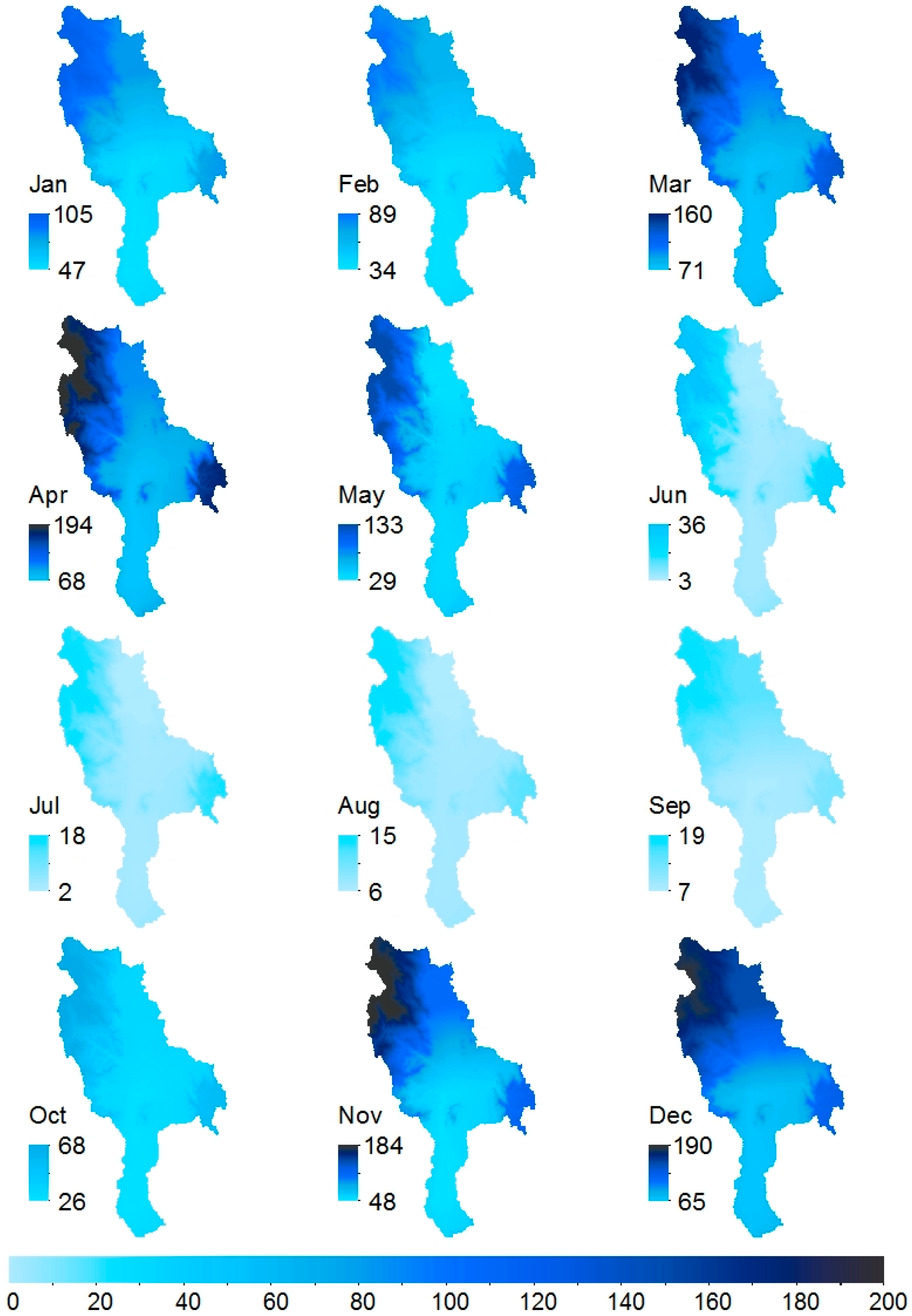
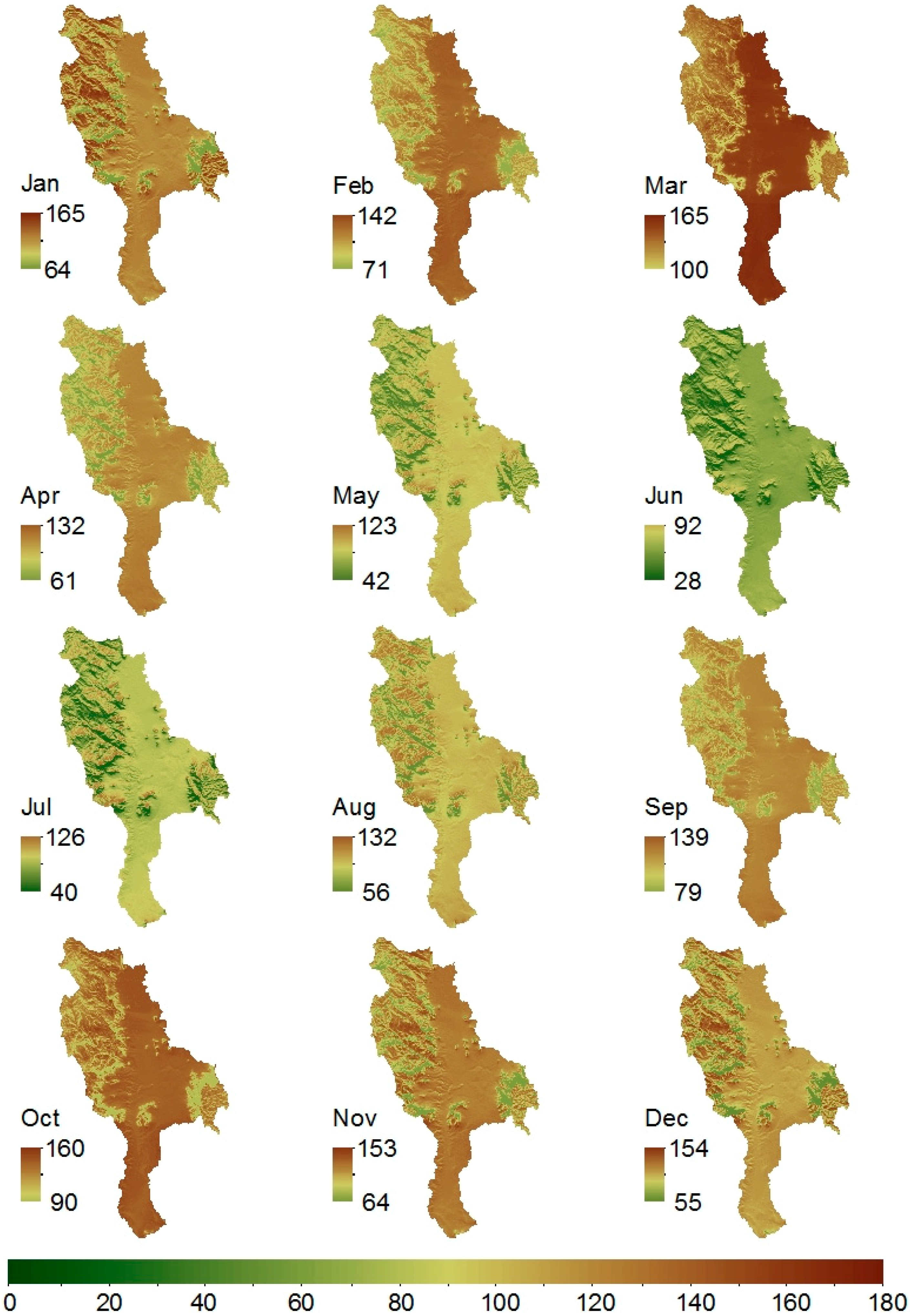
The constructed rainfall maps showed that monthly rainfall ranged from 2 mm along the valley to 194 mm on mountains (Figure 2). The results also showed that rainfall was abundant for the long-rains season in March–May centered in April. Nevertheless, during such periods mountain areas received more rainfall than in the valleys. In contrast, rainfall during the short-rains season in October–December revealed higher spatial variability in the leeward-side than in the windward-side. The valley in the windward-side received rainfall amounts similar as on mountains, particularly for the period November to December.

The number of temperature records available within the study area was very low. Therefore, it was necessary to include nearby meteorological stations to increase our understanding of the temperature gradient, which resulted in highly satisfactory estimations for this variable, as shown by high R² values. However, although maximum and minimum temperatures are commonly more easily modelled than rainfall because of low measurements uncertainties, the very high R² values for temperature were influenced by the little number of temperature stations used to model these climatic variables. These few stations were located in high altitudes and low altitudes, which supported a linear relation.

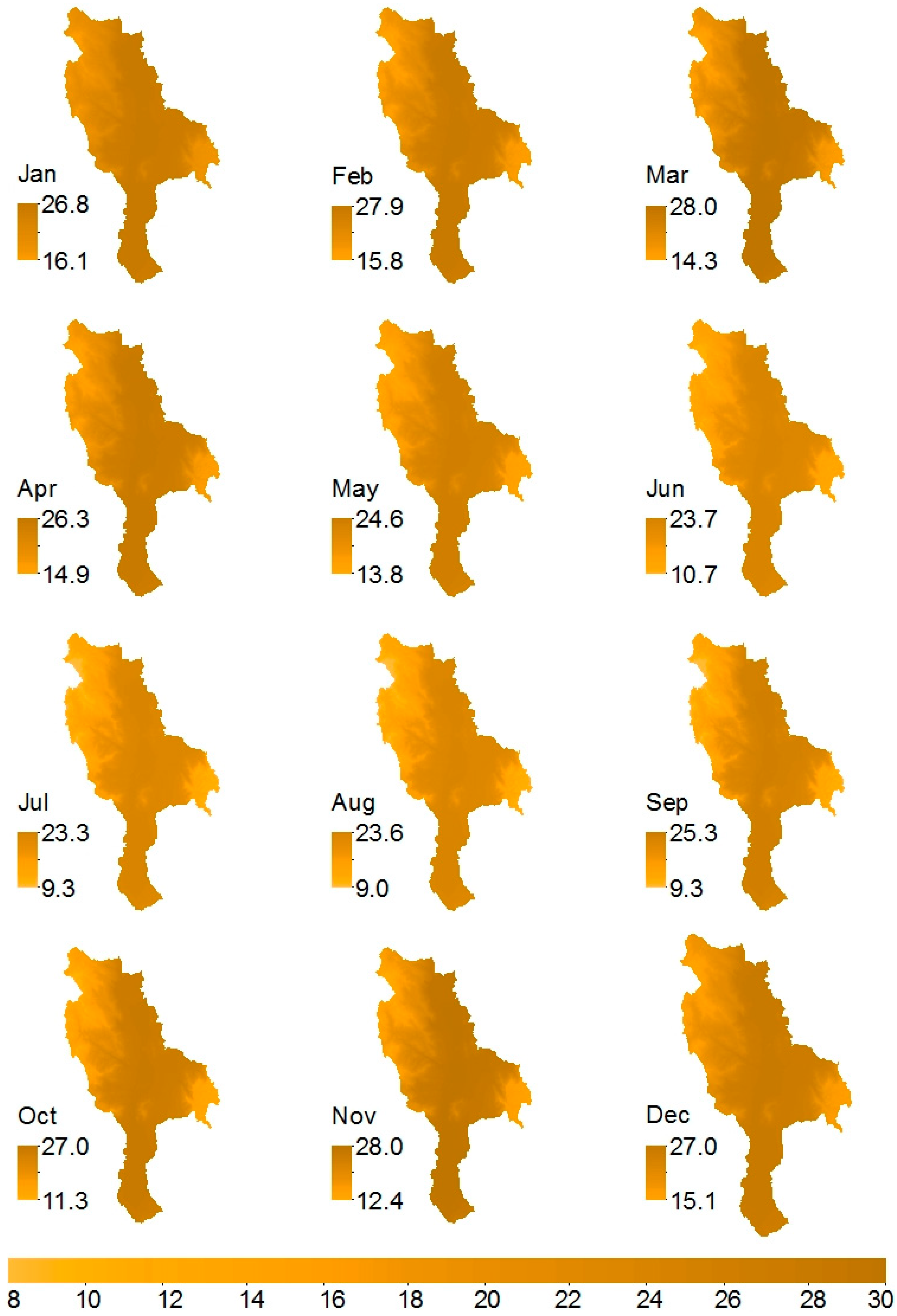
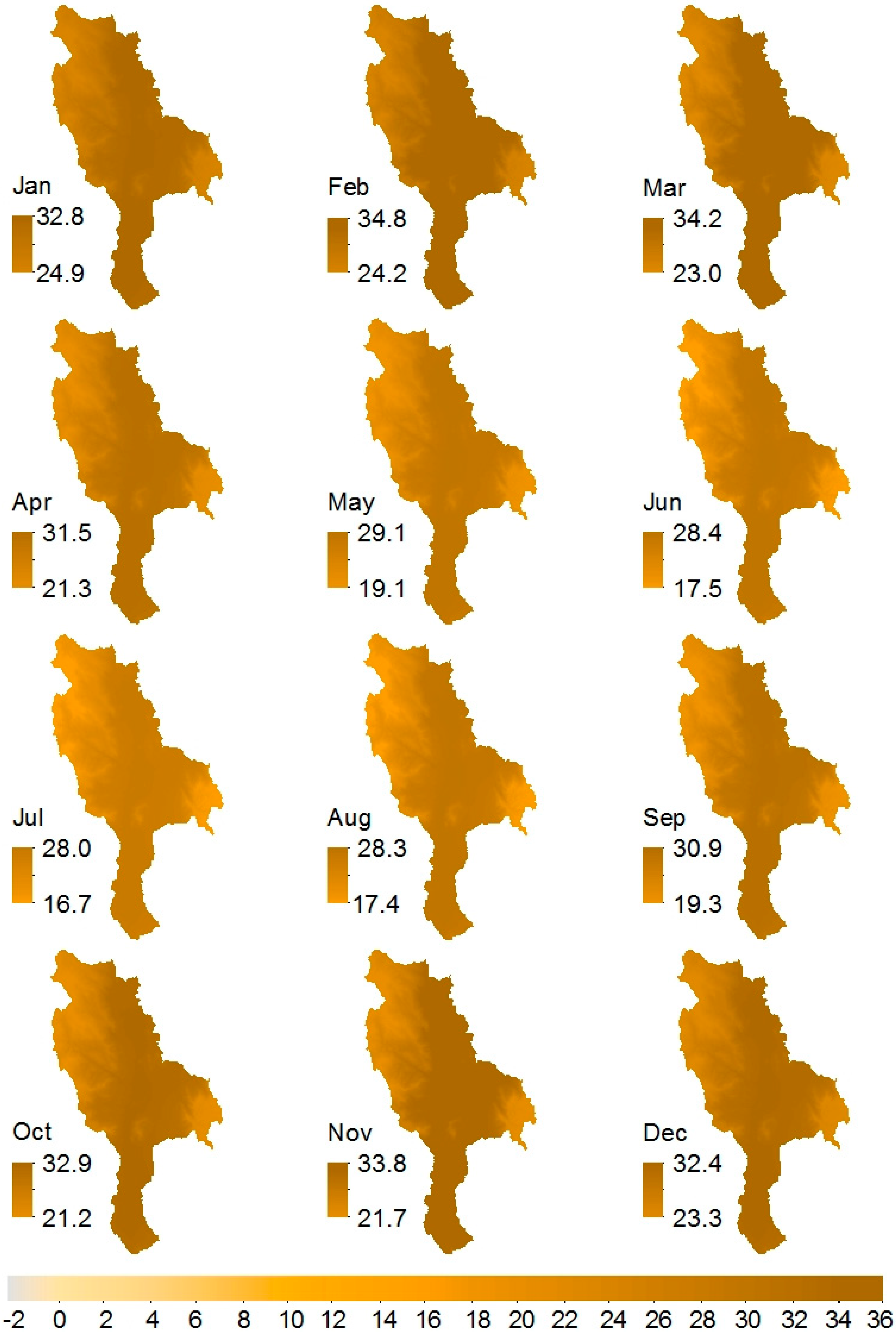
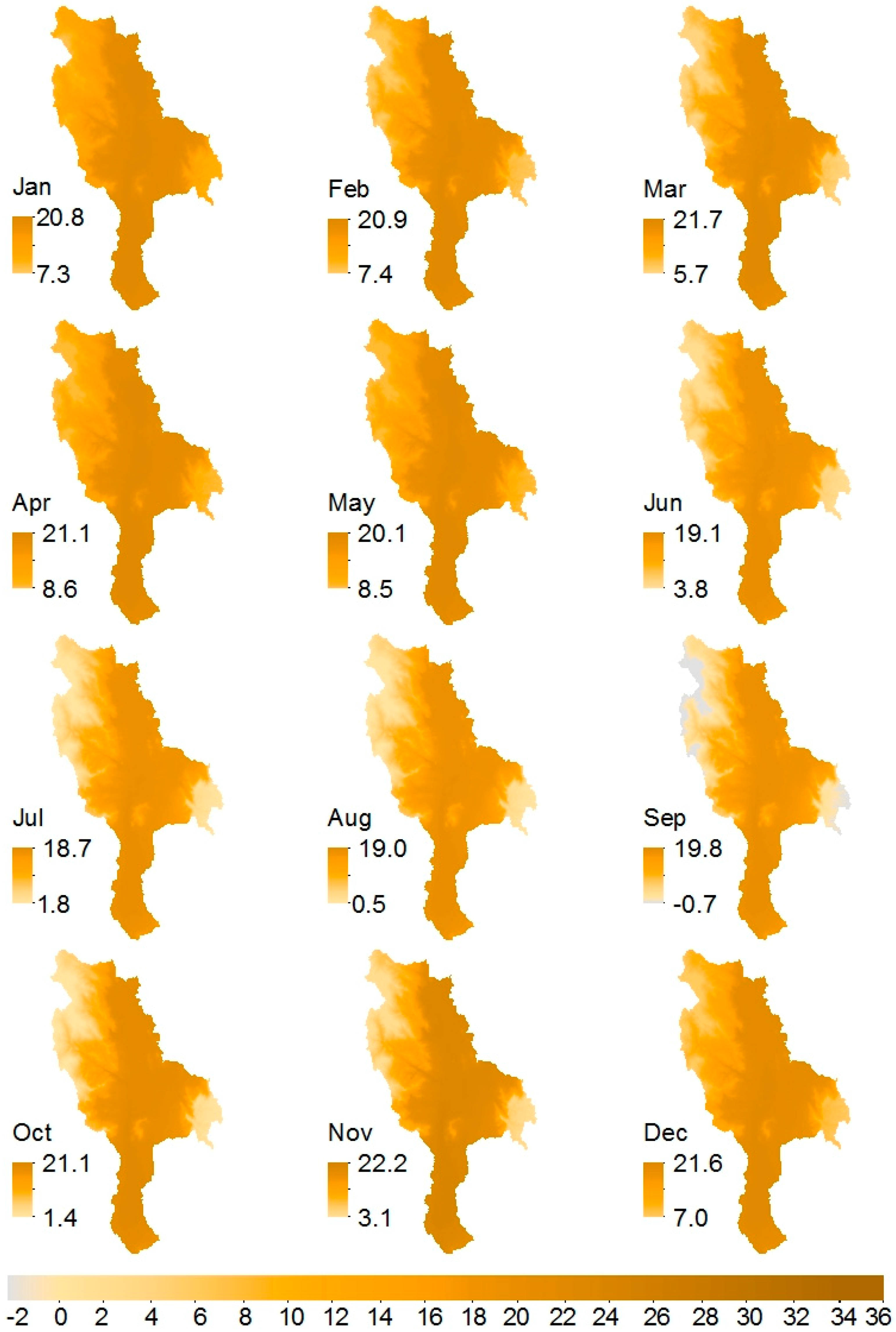
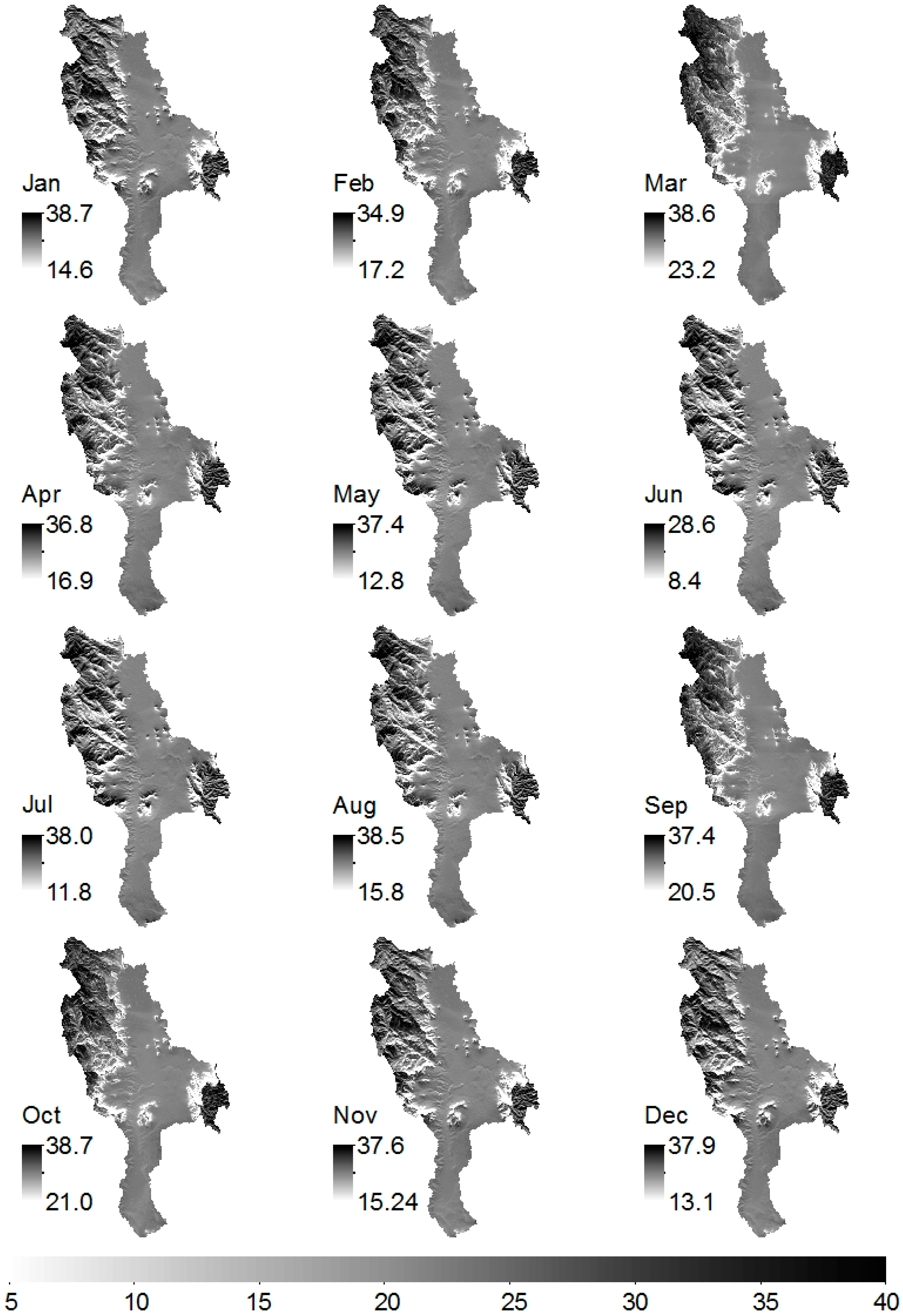
Mean monthly temperature strongly decreased with altitude, as expected (Figure 3). This effect was most pronounced in June–September, whereas the valley was characterized by similar temperatures throughout the year. The mean temperatures ranged from 9 °C (July–September) to 28 °C (February, March, and November). The period December–February was warmer where the temperature in the South Pare and West Usambara mountains was above 15 °C. Figure 3 also showed that the temperature was lower in July–September, particularly in higher altitudes. Moreover, the results showed that temperature in the Mkomazi valley was higher than 23 °C throughout the year. Maximum and minimum temperatures ranged from −1 to 35 °C (Figure 4 and Figure 5) with patterns and trends similar to that described for mean temperature.

The constructed monthly ET_o maps values ranged from 28 to 165 mm (Figure 6). Results showed that except for the period May–July, ET_o surpassed 50 mm, and was greater than 150 mm in January, March, and October–December, and below 150 mm in February, April, August, and September. In May–July ET_o ranged between 40 and 126 mm. Maximum ET_o occurred in March in which the lowest was 100 mm. In general, ET_o decreases with altitude. The results also showed that in January, November, and December some slopes had greater amounts of ET_o than on the plains, which primarily was associated with the effects of seasonal variations in the position of the sun on the slopes than on the plains. The constructed monthly extraterrestrial radiation maps are shown in Figure 7.

4. Discussion

In agronomic studies, calculations of reference evapotranspiration (ET_o) following the Hargreaves and Samani (HS) equation are generally performed using values of extraterrestrial radiation (R_a) calculated assuming a planar surface and solely as a function of latitude, according to the method described by Reference [4], which does not take relief into account. This study reveals the potential of regression-based models, digital elevation models (DEM), and geographic information systems (GIS) modelling techniques to map ET_o, precipitation and temperature—the climate variables that are important in many environmental and water resources studies [1,2,3]. We have modelled R_a using DEM and ArcGIS. The usefulness of this approach might not be for flat terrain, in which relief does not significantly affect R_a. However, in complex terrain, for high-resolution ET_o maps used for ecological and water resources management, spatial variations in relief are commonly very important and significantly affect the values of R_a estimates because radiation flux are especially dependent on the geometry of terrain [15], and this has a significant effect on local ET_o values [45].

The dataset was collected from many institutions, and cleaned for inhomogeneous data. Obvious outliers were removed by means of traditional methods based on the mean and standard deviation and a predefined limit. The largest risk of making a type I error (i.e., erroneously removing good data) was in the subjective decision to remove too high rainfall in dry months for dry years.

There was an overall relationship between elevation and both rainfall and temperature, as expected. The results of the precipitation models showed that, for the long-rains season in March–May, R² values for the period March–April increased for leeward and windward, and were great in April for both sides, in which rainfall peaked in April. In contrast, for short-rains season in October–December, in which rainfall peaked in December, R² values decreased and were very low in December. From the constructed rainfall maps and the analysis of temporal rainfall variability, precipitation patterns regimes agreed well with results from equatorial East African studies showing that the rainfall is abundant in most areas for the long-rains season [17], while short-rains season reveal more interannual variability [18]. High and low R² values corresponded with the temporal patterns in rainfall variability.

Rainfall was modelled in a linear form assuming that condensed water falls immediately to the ground and no influence of horizontal movements was included, which is somewhat violating mountain wave theory for modelling orographic precipitation [36]. It does not include the physical elements such as airflow dynamics, advection and fallout, condensed water convection, and downslope evaporation [46]. However, it is a usable assumption to obtain a relationship between elevation and precipitation in most situations, an example showing such an assumption is shown in the study by References [13]. In addition to general usable assumptions on climatic model development, one has to increase the complexity and performance of such models upon availability of other parameters.

An attempt to improve R² values for rainfall was to exclude stations at the ridge (station 9 in this case) for analysis of elevation–rainfall relationship and seasonal trends. The results showed significant improvement of R² values for windward-side, particularly for the short-rains season in comparison to the long-rains season. In contrast, there was no significant improvement of R² values for the leeward-side, particularly in December. Also, the elevation-rainfall relationship for the long-rains season for both windward and leeward models showed no significant R² differences with or without station 9. Low R² values indirectly indicate climate mechanisms for rainfall distribution in particular for the period November to January. The rainfall distribution form during this period is yet unknown. However, the climate of the Mkomazi River Basin is largely influenced by equatorial East African climate systems. Slingo and others [19] noted that over the Western Indian Ocean the inter-tropical convergence zone (ITCZ) makes its greatest North–South excursions, dominated by the Asian monsoon with its reversals of the wind from northeasterly in December–February to southwesterly in June–August periods. As such, during the transition periods in March–May as the northeast monsoon relaxes, the ITCZ from its southernmost position over the southern Western Indian Ocean progresses northwards bringing equatorial East Africa long-rains season, and as the Asian summer monsoon retreats in September–November, the ITCZ progresses South again bringing equatorial East Africa short-rains season. Therefore, we considered local prevailing winds, especially their trend and strength, associated with the ITCZ excursions, also to be an important variable for rainfall patterns.

We used the HS method to map ET_o for the reason that, to construct reliable maps, it is necessary to use a dense dataset of the climatic variables. Although the most accurate method is the one that is physically based on the Penman–Monteith equation, it is impossible to produce reliable ET_o maps using the Penman–Monteith equation in the area of data scarcity because of a relatively high data demand of such an equation. Apart from our specific study area, this may be the case for many Africa regions. In addition, numerous researchers (e.g., [41,47]) have demonstrated that, for ET_o estimates for periods longer than one week, the HS method provides similar results to those obtained using the Penman–Monteith equation.

As a caveat to our study, we note that the lack of climate stations and the sometimes discontinuous maintenance of the existing stations pose a serious obstacle to the derivation of climate maps from data. A small number of stations and the unavailability of additional climate parameters besides rainfall decrease the reliability of the regression functions that relate rainfall and temperature to elevation. Climate maps derived from sparse data must therefore considered with care. This problem will likely persist in the near future in many parts of sub-Saharan Africa.

5. Conclusions

Our study has demonstrated the potential use of linear-regression-based, digital elevation models (DEM), and geographic information systems (GIS) techniques in modelling and construction of reliable climate maps. These maps were made on a monthly basis for rainfall, temperatures, and evapotranspiration.

Both rainfall and temperature showed a linear correlation form with elevation. Temperature linear correlation form with elevation was stronger than that showed by rainfall with elevation. These temperature stations were located on two different altitudes (low and high), which supported the linear form strongly. For rainfall, the linear form was more pronounced for the long-rains seasons than for the short-rains season. For the long-rains season, the rainfall-elevation relationships showed no significant changes in R² values, both for the leeward- and windward-side, when the station at the ridge was not included for the analysis of rainfall–elevation relationship. In contrast, for the short-rains season, R² values improved substantially when station at the ridge was not included into rainfall models. Therefore, rainfall distribution for the southern Mkomazi River Basin particularly for the short-rains season deserves further attention, when other variables affecting rainfall distribution (e.g., wind speed and direction) become available.

The constructed maps for reference evapotranspiration (ET_o), rainfall, and temperatures can be useful for environment and water resources studies in the region as climate variability affects river flows, which has in turn implications on livelihoods of the people which depend directly or indirectly on rain-fed agriculture.

References

- Trenberth, K.E.; Smith, L.; Qian, T.T.; Dai, A.; Fasullo, J. Estimates of the Global Water Budget and Its Annual Cycle Using Observational and Model Data. J. Hydrometeorol. 2007, 8, 758–769. [Google Scholar] [CrossRef] [Green Version]
- Ward, A.D.; Trimble, S.W. Environmental Hydrology, 2nd ed.; CRC Press: Boca Raton, FL, USA, 2003; pp. 1–118. ISBN 1566706165. [Google Scholar]
- Mu, Q.; Heinsch, F.A.; Zhao, M.; Running, S.W. Development of a global evapotranspiration algorithm based on MODIS and global meteorology data. Remote Sens. Environ. 2007, 111, 519–536. [Google Scholar] [CrossRef]
- Allen, R.G.; Pereira, L.S.; Raes, D.; Smith, M. Crop Evapotranspiration: Guidelines for Computing Crop Water Requirements; Irrigation and Drainage Paper 56; Food and Agriculture Organization: Rome, Italy, 1998; pp. 26–40. [Google Scholar]
- Barry, R.G. Mountain Weather & Climate, 2nd ed.; Routledge: New York, NY, USA, 1992; pp. 1–180. ISBN 0415071127. [Google Scholar]
- Diaz, H.F. Climate Variability and Change in High Elevation Regions: Past, Present & Future, 1st ed.; Kluwer Academic Publishers: Dordrecht, The Netherlands, 2003; pp. 1–4. ISBN 1402013868. [Google Scholar]
- Whiteman, C.D. Mountain Meteorology: Fundamentals and Applications, 1st ed.; Oxford University Press: New York, NY, USA, 2000; pp. 3–204. ISBN 0195132718. [Google Scholar]
- Li, J.; Heap, A.D. A Review of Spatial Interpolation Methods for Environmental Scientists, 1st ed.; Geoscience Australia: Canberra, Australia, 2008; pp. 4–95. ISBN 1921498307. [Google Scholar]
- Goovaerts, P. Geostatistics for Natural Resources Evaluation, 1st ed.; Oxford University Press: New York, NY, USA, 1997; pp. 125–436. ISBN 0195115384. [Google Scholar]
- Mair, A.; Fares, A. Comparison of Rainfall Interpolation Methods in a Mountainous Region of a Tropical Island. J. Hydrol. Eng. 2011, 16, 371–383. [Google Scholar] [CrossRef]
- Martínez-Cob, A. Multivariate geostatistical analysis of evapotranspiration and precipitation in mountainous terrain. J. Hydrol. 1996, 174, 19–35. [Google Scholar] [CrossRef] [Green Version]
- Chapman, L.; Thornes, J.E. The Use of Geographic Information Systems in Climatology and Meteorology. Prog. Phys. Geogr. 2003, 27, 313–330. [Google Scholar] [CrossRef]
- Daly, C.; Neilson, R.P.; Phillips, D.L. A Statistical-Topographic Model for Mapping Climatological Precipitation over Mountainous Terrain. J. Appl. Meteorol. 1994, 33, 140–158. [Google Scholar] [CrossRef] [Green Version]
- Gómez, J.; Etchevers, J.; Monterroso, A.; Gay, C.; Campo, J.; Martínez, M. Spatial estimation of mean temperature and precipitation in areas of scarce meteorological information. Atmosfera 2008, 21, 35–56. [Google Scholar]
- Vicente-Serrano, S.M.; Lanjeri, S.; Lopez-Moreno, J. Comparison of different procedures to map reference evapotranspiration using geographical information systems and regression-based techniques. Int. J. Climatol. 2007, 27, 1103–1118. [Google Scholar] [CrossRef] [Green Version]
- Basist, A.; Bell, G.D.; Meentemeyer, V. Statistical Relationships between Topography and Precipitation Patterns. J. Clim. 1994, 7, 1305–1315. [Google Scholar] [CrossRef] [Green Version]
- Camberlin, P.; Philippon, N. The East African March-May Rainy Season: Associated Atmospheric Dynamics and Predictability over the 1968–97 Period. J. Clim. 2002, 15, 1002–1019. [Google Scholar] [CrossRef]
- Mutai, C.C.; Ward, M.N. East African Rainfall and the Tropical Circulation/Convection on Intraseasonal to Interannual Timescales. J. Clim. 2000, 13, 3915–3939. [Google Scholar] [CrossRef]
- Slingo, J.; Spencer, H.; Hoskins, B.; Berrisford, P.; Black, E. The meteorology of the Western Indian Ocean, and the influence of the East African Highlands. Philos. Trans. Ser. A Math. Phys. Eng. Sci. 2005, 363, 25–42. [Google Scholar] [CrossRef] [PubMed]
- Kijazi, A.L.; Reason, C.J.C. Relationships between intraseasonal rainfall variability of coastal Tanzania and ENSO. Theor. Appl. Climatol. 2005, 82, 153–176. [Google Scholar] [CrossRef]
- Saji, N.H.; Goswami, B.N.; Vinayachandran, P.N.; Yamagata, T. A dipole mode in the tropical Indian Ocean. Nature 1999, 401, 360–363. [Google Scholar] [CrossRef] [PubMed]
- Fischer, A.S.; Terray, P.; Guilyardi, E.; Gualdi, S.; Delecluse, P. Two Independent Triggers for the Indian Ocean Dipole/Zonal Mode in a Coupled GCM. J. Clim. 2005, 18, 3428–3449. [Google Scholar] [CrossRef] [Green Version]
- Latif, M.; Dommenget, D.; Dima, M.; Grotzner, A. The Role of Indian Ocean Sea Surface Temperature in Forcing East African Rainfall Anomalies during December–January 1997/98. J. Clim. 1999, 12, 3497–3504. [Google Scholar] [CrossRef] [Green Version]
- Hastenrath, S.; Polzin, D.; Mutai, C. Diagnosing the 2005 Drought in Equatorial East Africa. J. Clim. 2007, 20, 4628–4637. [Google Scholar] [CrossRef]
- Bjørndalen, J.E. Tanzania’s vanishing rain forests—Assessment of nature conservation values, biodiversity and importance for water catchment. Agric. Ecosyst. Environ. 1992, 40, 313–334. [Google Scholar] [CrossRef]
- PBWO; IUCN. Pangani River System; State of the Basin Report; PWBO: Moshi, Tanzania; IUCN Eastern Africa Regional Program: Nairobi, Kenya, 2007. [Google Scholar]
- Xu, C.Y.; Tunemar, L.; Chen, Y.Q.D.; Singh, V.P. Evaluation of seasonal and spatial variations of lumped water balance model sensitivity to precipitation data errors. J. Hydrol. 2006, 324, 80–93. [Google Scholar] [CrossRef]
- Dingman, S.L.; Seelyreynolds, D.M.; Reynolds, R.C. Application of Kriging to Estimating Mean Annual Precipitation in a Region of Orographic Influence. Water Resour. Bull. 1988, 24, 329–339. [Google Scholar] [CrossRef]
- Reek, T.; Doty, S.R.; Owen, T.W. A Deterministic Approach to the Validation of Historical Daily Temperature and Precipitation Data from the Cooperative Network. Am. Meteorol. Soc. 1992, 73, 753–762. [Google Scholar] [CrossRef] [Green Version]
- Feng, S.; Hu, Q.; Qian, W. Quality Control of Daily Meteorological Data in China, 1951–2000: A New Dataset. Int. J. Climatol. 2004, 24, 853–870. [Google Scholar] [CrossRef]
- Begert, M.; Schlegel, T.; Kirchhofer, W. Homogeneous Temperature and Precipitation Series of Switzerland from 1864 to 2000. Int. J. Climatol. 2005, 25, 65–80. [Google Scholar] [CrossRef]
- Keiser, D.T.; Griffiths, J.F. Problems Associated with Homogeneity Testing in Climate Variation Studies: A Case Study of Temperature in the Northern Great Plains, USA. Int. J. Climatol. 1997, 17, 497–510. [Google Scholar] [CrossRef]
- Mitchell, T.D.; Jones, P.D. An Improved Method of Constructing a Database of Monthly Climate Observations and Associated High-Resolution Grids. Int. J. Climatol. 2005, 25, 693–712. [Google Scholar] [CrossRef]
- Lanzante, J.R. Resistant, Robust and Non-Parametric Techniques for the Analysis of Climate Data: Theory and Examples, Including Applications to Historical Radiosonde Station Data. Int. J. Climatol. 1996, 16, 1197–1226. [Google Scholar] [CrossRef]
- Shiffler, R.E. Maximum Z-Scores and Outliers. Am. Stat. 1988, 42, 79–80. [Google Scholar]
- Smith, R.B. The Influence of Mountains on the Atmosphere. Adv. Geophys. 1979, 21, 87–230. [Google Scholar]
- Jiang, Q.F. Moist dynamics and orographic precipitation. Tellus 2003, 55, 301–316. [Google Scholar] [CrossRef]
- Ninyerola, M.; Pons, X.; Roure, J.M. Monthly precipitation mapping of the Iberian Peninsula using spatial interpolation tools implemented in a Geographic Information System. Theor. Appl. Climatol. 2007, 89, 195–209. [Google Scholar] [CrossRef] [Green Version]
- Marquinez, J.; Lastra, J.; Garcia, P. Estimation models for precipitation in mountainous regions: The use of GIS and multivariate analysis. J. Hydrol. 2003, 270, 1–11. [Google Scholar] [CrossRef]
- Hargreaves, G.H.; Samani, Z.A. Reference Crop Evapotranspiration from Temperature. Appl. Eng. Agric. 1985, 1, 96–99. [Google Scholar] [CrossRef]
- Droogers, P.; Allen, R.G. Estimating reference evapotranspiration under inaccurate data conditions. Irrig. Drain. Syst. 2002, 16, 33–45. [Google Scholar] [CrossRef]
- Fu, P.D.; Rich, P.M. A geometric solar radiation model with applications in agriculture and forestry. Comput. Electron. Agric. 2002, 37, 25–35. [Google Scholar] [CrossRef]
- Draper, N.R.; Smith, H. Applied Regression Analysis, 3rd ed.; John Wiley & Sons: New York, USA, 1998; Volume 1, pp. 15–460. ISBN 0471170828. [Google Scholar]
- Kotz, S.; Balakrishnan, N.; Johnson, N.L. Continuous Multivariate Distributions: Models and Applications, 2nd ed.; John Wiley & Sons: New York, NY, USA, 2004; Volume 1, ISBN 0471654035. [Google Scholar]
- Häntzschel, J.; Goldberg, V.; Bernhofer, C. GIS-based regionalisation of radiation, temperature and coupling measures in complex terrain for low mountain ranges. Meteorol. Appl. 2005, 12, 33–42. [Google Scholar] [CrossRef] [Green Version]
- Smith, R.B.; Barstad, I. A Linear Theory of Orographic Precipitation. J. Atmos. Sci. 2004, 61, 1377–1391. [Google Scholar] [CrossRef]
- Hargreaves, G.H.; Allen, R.G. History and Evaluation of Hargreaves Evapotranspiration Equation. J. Irrig. Drain. Eng.-ASCE 2003, 129, 53–63. [Google Scholar] [CrossRef]
Figure 1.
A map shows the location of the Mkomazi River Basin (Tanzania), which is the sub-catchment of the Pangani River Basin.
Figure 2.
Monthly mean rainfall (mm) maps for the southern Mkomazi River Basin averaged for the period 1964–2010.
Figure 3.
Monthly mean temperature (°C) maps for the southern Mkomazi River Basin averaged for the period 1989–1994.
Figure 4.
Monthly averaged maximum temperature (°C) maps for the southern Mkomazi River Basin for the period 1989–1994.
Figure 5.
Monthly averaged minimum temperature (°C) maps for the southern Mkomazi River Basin for the period 1989–1994.
Figure 6.
Monthly reference evapotranspiration (mm) maps for the southern Mkomazi River Basin averaged for the period 1989–1994.
Figure 7.
Monthly extraterrestrial radiation (MJ m−2 day−1) for the southern Mkomazi River Basin.