Wing Tip Drag Reduction at Nominal Take-Off Mach Number: An Approach to Local Active Flow Control with a Highly Robust Actuator System

Abstract

This paper discusses wind tunnel test results aimed at advancing active flow control technology to increase the aerodynamic efficiency of an aircraft during take-off. A model of the outer section of a representative civil airliner wing was equipped with two-stage fluidic actuators between the slat edge and wing tip, where mechanical high-lift devices fail to integrate. The experiments were conducted at a nominal take-off Mach number of M = 0.2. At this incidence velocity, separation on the wing section, accompanied by increased drag, is triggered by the strong slat edge vortex at high angles of attack. On the basis of global force measurements and local static pressure data, the effect of pulsed blowing on the complex flow is evaluated, considering various momentum coefficients and spanwise distributions of the actuation effort. It is shown that through local intensification of forcing, a momentum coefficient of less than $c_{\mu }=0.6\%$ suffices to offset the stall by 2.4°, increase the maximum lift by more than 10% and reduce the drag by 37% compared to the uncontrolled flow.

1. Introduction

The design of wing tip devices on civil airliners has changed remarkably in past decades. The conception of wing tip devices dates back more than a century, with the first functioning design patented in 1915 [1] by W. E. Somerville, describing a “Flying-machine” with wings of which “... the extreme end is curved upward”. However, it was not until the research of Whitcomb [2] 60 years later, triggered by an energy crisis that resulted in the need for better fuel performance, that wing tip devices found their way into practice. Winglets (and all derivatives thereof) are designed to minimize the drag during cruise flight. This approach conflicts with performance requirements during low-speed flight when a high-lift system is needed, as the slender shape and high local curvature of modern wing tip devices inhibit the integration of a slat, resulting in early separation at the wing tip at high angles of attack. This optimization conflict might be resolved by active flow control (AFC), as this technology has the potential to augment the overall high-lift system to prevent flow separation where the integration of mechanical devices fails. The suppression of local flow separation is most relevant during the second segment of climb (cf. Federal Aviation Regulations (FAR) Part 25), when the landing gear is retracted and a minimum gradient of climb is prescribed even with one engine inoperative. In [3], the climb gradient $tan\left(\gamma \right)$ is defined as a function of the available thrust (T), aircraft weight (W) and aerodynamic efficiency, which is the ratio of the lift (L) and drag (D):

$$tan\left(\gamma \right)=\frac{T}{W}-\frac{1}{(L/D)}$$

Increasing the lift-to-drag ratio ($\frac{L}{D}$) by local flow control would make it possible to reduce the installed thrust (use smaller engines) or to increase the maximum take-off weight (realize higher passenger capacity).

In this paper, we report the results of wind tunnel experiments conducted on a realistic outer wing model at the nominal take-off Mach number of M = 0.2, with local flow control applied between the outer slat edge and wing tip. Pulsed blowing is employed to increase the wing model’s aerodynamic efficiency by offsetting the increase in drag. The feasibility of preventing separation at the leading edge by AFC was demonstrated successfully in recent studies [4,5,6,7,8,9,10], which focused primarily on increasing the maximum lift and stall angle of slatless single- or multi-element airfoils. Research on localized flow control has also appeared in a multidisciplinary study from the aeronautical industry [11]. Most researchers resort to unsteady excitation of the flow, as this was found to be more efficient than, e.g., steady blowing [12]. Our flow control system relies on fluid amplifier components, which were first studied at the Harry Diamond Laboratories in the early 1960s [13] and have resurfaced in the form of flow control actuators in recent years, as their robustness and simplicity make them a candidate technology for transfer into industry applications. A review of different types of fluid amplifiers, and their application for flow control is given in [14]. Impressive results were obtained using this actuator type, e.g., in experiments to improve the rudder effectiveness of a full-scale vertical tail plane [15,16].

In this paper, we study the effect of the spanwise distribution of the actuation and investigate the effect of the momentum coefficient and jet velocity ratio on the aerodynamic performance of the outer wing model. Localized changes in the model’s wake flow field are analyzed using five-hole probe data gathered downstream of the model, and the net benefit of controlling the flow is quantified in terms of the first aerodynamic figure of merit. We show that with a suitable combination of control parameters, we can reduce the drag at the maximum angle of attack by 37% compared to the base flow value while increasing the maximum lift by more than 10%.

2. Experimental Setup

This section describes the wind tunnel model, including the fluidic actuator system, and specifies the experimental uncertainty.

2.1. Wind Tunnel Model and Instrumentation

The experiments were conducted on the model of an outer wing section representative of a modern civil aircraft (see Figure 1). The inner third of the model is equipped with a leading edge slat and an aileron deflected to the take-off configuration. Adjacent to this, a highly three-dimensional wing tip device optimized for cruise flight is mounted. This part of the wing model is not protected by a slat. The model measures approximately 1400 mm from wind tunnel floor to wing tip. A peniche (164 mm in height) and a splitter plate, which are employed to reduce the effect of the wind tunnel floor boundary layer and which are not connected to the balance system, reduce the effective span b of the model to 1250 mm. The test campaign was conducted in the atmospheric large low-speed wind tunnel facility of DNW-NWB (Deutsch-Niederländische Windkanäle - Niedergeschwindigkeits-Windkanal Braunschweig, German accronym for: German-Dutch Wind Tunnels, Low-Speed Wind Tunnel Braunschweig) in a 3.25 m × 2.8 m × 8.0 m closed test section. The investigations were performed at a typical take-off Mach number of M = 0.2. The resulting Reynolds number based on the model’s reference chord length $c_{ref}$ of 490 mm is $Re\approx 2\times {10}^6$. The forces and moments acting on the model were measured using a six-component balance system mounted beneath the wind tunnel floor. Rotating the balance with the model made it possible to vary the incidence angle. Static pressure data were acquired in six chordwise and three spanwise sections totaling more than 150 pressure taps. Tufts in combination with high-resolution cameras were used to monitor the surface flow on the suction side of the model wing. The topology of the model wake was measured with a traversable five-hole probe rake positioned at a constant x position downstream of the swept model, which results in a locally variable downstream distance from the trailing edge between $0.5c_{ref}$ and $1.5c_{ref}$. The rake consists of 18 equidistant probes. The flow field investigated spans $0.15<y/b<0.85$ in the y direction and is $\mathrm{\Delta }z/b=0.4$ wide. The spatial resolution of the data points is 15 mm in both directions.

2.2. Active Flow Control System

The flow control system (see Figure 2) is located between $y/b=40\%$ and $y/b=75\%$ of the model’s span. Its design is based on experience from numerical and experimental studies on a similar geometry [17,18]. A total of 28 rectangular slots are integrated parallel to the leading edge at $x/c_{ref}\approx 5\%$ on the suction-side surface. Each slot measures 12.4 mm in the spanwise direction and 0.88 mm in the chordwise direction. The gap between two neighboring outlets is approximately 3.1 mm. Through those slots, compressed air is ejected periodically. The air jets are tilted by ${30}^{°}$ relative to the model’s surface. The outlets are grouped into three segments with a design-related spacing of 15 mm between them.

The pulsed air jets required for the flow control approach pursued in this paper are generated using fluidic elements based on the principle of fluid amplification. Those devices make it possible to switch the primary jet between two stable states by applying a much weaker (in terms of lower momentum and mass flow rate) control jet. The flow control system employed here follows the two-stage approach presented in [9] and consists of a fluidic oscillator acting as the driving stage and an array of five (Segments S1 and S2) or four (Segment S3) fluidic diverter elements acting as the outlet stage. Within the driving stage, a feedback mechanism causes the flow to switch periodically between two branches when fluid passes through it. Each branch has outlets connected to the second stages’ control ports, providing this stage with the required control signal. In turn, this pneumatic control signal switches the flow in the second stage between the two corresponding outlets of one diverter element. This results in a pulsed jet flow in which neighboring air jets have a phase shift of ${180}^{°}$. As switching between the outlets of one diverter is induced by the mass flow that propagates through the branches of the control stages, there is a phase lag in switching between two neighboring actuator elements in one segment. The air pressure supply for each segment’s first and second stages is controlled independently by a pressure regulator valve, allowing different forcing amplitudes across the segments and fine-tuning of the actuation frequency. Mass flow meters based on the thermoelectric principle are used to measure the flow rate of the ejected air for each actuator array. The frequency of actuation was determined using Kulite pressure transducers installed in the AFC system’s driving stages during the experiments. The system performance was evaluated before the wind tunnel testing to ensure a sufficiently homogeneous jet velocity distribution along the span. For that purpose, the total pressure along the centerline of each outlet was measured with a Pitot tube connected to a Kulite pressure transducer. The peak total pressure measured at the individual outlets lies within ±2% of the average peak value recorded across all outlets. To illustrate the switching quality of the actuators, the time history of the total pressure data recorded at the center of one outlet of Segment S1 is provided in Figure 3, demonstrating fully modulated operation.

As this flow control system incorporates no moving or electrical components, the switching frequency depends only on the mass flow rates through the driving and outlet stages and the ratio thereof. An example of a map of this correlation is shown in Figure 4.

All of the quoted momentum coefficients are calculated using $c_{\mu }=\frac{\dot{m}·u_{jet,RMS}}{q_{\infty }·A_{ref}}$, where $u_{jet,RMS}$ is the RMS value of the peak jet velocity. Introducing the simplifying, rough assumptions of a uniform velocity profile (plug flow) across the outlet, and the form of a square wave signal in time, $u_{jet,RMS}$, can be approximated by $u_{jet,RMS}=\sqrt{DC}·u_{jet,peak}$. The duty cycle (DC) describes the fraction of time one outlet is active during one switching cycle. It is fixed at 50% (DC = 0.5) in our studies. The peak jet velocity $u_{jet,peak}$ is calculated from the measured mass flow rate ($\dot{m}$), the area of the active actuator outlets ($A_{AFC}$) and the density of the fluid at the outlets (${\rho }_{jet}$), using $u_{jet,peak}=\frac{\dot{m}}{{\rho }_{jet}{A}_{AFC}}$. The jet densities for different mass flow rates were established in bench-top experiments. A more detailed description of the $c_{\mu }$ calculation is found in [18]. When multiple segments were active, the $c_{\mu }$ value quoted is the sum of the values for each active segment.

2.3. Experimental Uncertainty

The uncertainty in measuring forces with the balance system is 0.3% of each of the full scale spans, which are 2000 N for the drag and 8100 N for the lift. This translates to an uncertainty of less than $\mathrm{\Delta }{C}_L\pm 0.007$ in the lift coefficient and of less than $\mathrm{\Delta }{C}_D\pm 0.002$ in the drag coefficient. The maximum expected error in measuring the pressure is 0.1% of the full span ranges of the pressure transducers, which are 5 psi and 15 psi for static pressure on the model and 5 psi for the five-hole probe wake rake. The results presented are corrected for wind tunnel effects using the method described in [19]. The momentum coefficient is calculated from the mass flow rate through the outlet slots measured in situ during the experiments and the jet density at the outlets, which was determined in bench-top experiments. The deviation of the quoted momentum coefficients from the exact values is determined by the simplifying assumptions regarding the velocity profile in time and space and the measurement error in the mass flow rate and density. This (absolute) uncertainty is difficult to quantify. However, as the uncertainty in the density and velocity profiles produces a systematic error, the relative uncertainty between the various $c_{\mu }$ values quoted is determined only by the uncertainty in measuring the mass flow rate, which is specified as $\pm 1\%$ of the sensors’ full-scale range. This translates to an uncertainty in $\mathrm{\Delta }{c}_{\mu }$ of approximately $\pm 0.01\%$ per active segment.

3. Results

The major findings of our wind tunnel experiments are presented in this section. We describe the topology and separation behavior of the base flow and discuss the effects of flow control on the aerodynamic performance of the model wing. All of the aerodynamic coefficients are normalized by their respective base flow values, $c_{D,min,base}$, $c_{L,max,base}$ and ${(c_L/c_D)}_{max,base}$.

3.1. Discussion of Wind Tunnel and Mach Number Influences

The focus of the paper lies on the results obtained at the nominal take-off Mach number of $M=0.2$ in the DNW-NWB wind tunnel facility. However, prior to addressing those results, two aspects are considered in this subsection. Namely, the comparison of results across wind tunnels and the influence of the test Mach number. Experiments on a similar geometry with only slightly reduced geometric complexity, reported in [18], were conducted earlier in a wind tunnel of Technische Universität Berlin. In this test facility, the maximum Mach number is limited to $M=0.13$. The main difference in the experimental setup, however, is the ratio of the model size and wind tunnel cross-section, which is $\frac{A_{ref}}{A_{w/t,GroWiKa}}\approx 17\%$ for the results of [18] and $\frac{A_{ref}}{A_{w/t,DNW-NWB}}\approx 6\%$ for the DNW-NWB results. Figure 5 shows the drag coefficient curves with and without flow control for experiments conducted at $M=0.1$ in the two respective wind tunnels.

Note that the actuator system for all curves shown in this figure is the valve driven version from [18]. Despite the differences in wind tunnel size, the resulting drag coefficient curves for the uncontrolled flow agree remarkably well with respect to absolute (normalized) values and stall behavior. For the DNW-NWB results, stall occurs approximately $\mathrm{\Delta }\alpha \approx 0.5^{°}$ earlier, and the drag curve is shifted to slightly higher values. This might be attributed to increased tunnel size and the resulting reduced effect of the wind tunnel walls acting as guiding vanes on the flow above the wing. Analogously, the drag curves for the controlled flow are in good accordance for both facilities. The absolute values for the drag coefficient agree excellently up to high angles of attack. The flow control effectiveness is reduced slightly in the larger facility, which expresses itself as an reduction in stall offset from $\mathrm{\Delta }{\alpha }_{max}\approx 4^{°}$ to $\mathrm{\Delta }{\alpha }_{max}\approx 3.3^{°}$.

A more drastic effect is observed when increasing the incidence Mach number from $M=0.1$ to $M=0.2$ in the DNW-NWB wind tunnel facility, shown in Figure 6. Although, again, the absolute values for the drag coefficient curves agree well, the stall angle is increased by $\mathrm{\Delta }{\alpha }_{max}\approx 3^{°}$ for the higher incidence Mach number. In addition, the effectiveness of flow control is reduced significantly for the given valve-driven actuator setup. This effect is attributed to the massive change in stall behavior. At $M=0.1$, stall occurs outboard first and progresses gradually to the inboard section of the model. This process is delineated in detail in [18]. In contrast, stall is triggered by the increasing strength of the slat edge vortex for the higher Mach number, as will be shown in the following sections and illustrated specifically along the lines of several tuft flow visualization images when discussing the baseflow below. Thus, the comparison of the flow control effect between the two Mach numbers (and wind tunnels in consequence) is omitted, and the focus of discussion will be placed on the relevant take-off Mach number of $M=0.2$. Note, that for all results discussed below, the non-moving-parts’ two-stage flow control actuator system is employed, as it yields better control performance and is closer to potential industry application due to its higher robustness.

3.2. Base Flow

Because the model wing is three-dimensional, the base flow topology is highly complex and dominated by a strong outboard-directed cross-flow component over a wide range of incidence angles. Separation occurs locally at different angles of attack until the slat edge vortex has grown strong enough to induce flow separation in its vicinity, resulting in an almost instantaneous separation of the remaining attached flow on the slatless wing section. In this section, the separation process is described in terms of global force measurements, surface pressure data and surface tuft flow visualization, in order to revisit these findings later in light of our flow control attempts.

Figure 7 shows the lift and drag coefficients for the uncontrolled flow against the angle of attack. The lift increases linearly with increasing incidence angle up to the maximum angle of attack region, where the onset of separation reduces the slope of the lift curve and results in increased drag. For the selected angles of attack (marked in Figure 7), the pressure coefficient curves in the spanwise direction are shown in Figure 8.

The static pressure taps for which the data are plotted are located at the leading edge at $x/c=0\%$, which is near the suction peak for the incidence angles shown. The data are normalized with respect to the magnitude of the lowest recorded $c_p$ value. From these data, it is apparent that flow separation progresses from wing tip to wing root with increasing incidence. At a sufficiently low angle of attack (${\alpha }_1$), a suction peak manifests along the entire span, indicating attached flow. For increasing incidence (${\alpha }_1\to {\alpha }_4$), the magnitude of the $c_p$ values increases continuously in the portion of the span where there is attached flow. The static pressure on the surface is lowest downstream of the slat edge at $y/b\approx 0.45$. Concurrently, the fraction of the span where the flow separates at the leading edge and no suction peak is formed progresses inward, from $y/b\approx 0.9$ for ${\alpha }_1$ to $y/b\approx 0.7$ for ${\alpha }_4$. A further increase in the incidence angle (${\alpha }_5$) results in an abrupt separation on the entire unslatted (unprotected) section of the model wing, which causes a drop in $c_p$ at all of the stations plotted. This is confirmed in the tuft flow visualization presented in Figure 9, which shows the outer part of the wing model from $y/b=0.66$ to $y/b=1$.

For low incidence (${\alpha }_1$), the tufts indicate attached flow with a significant cross-flow component directed toward the wing tip. Increasing the angle of attack to ${\alpha }_2$ results in an even more prominent cross-flow component, a higher unsteadiness of the tufts in the aft region of the model and the onset of separation on the wing tip, as indicated by the orientation of the tufts. At ${\alpha }_3$, the flow on the part of the model shown in the figure is mostly separated, and the tufts show highly erratic motion and reversed orientation. At this angle of attack (${\alpha }_3$), which is just beyond ${\alpha }_{max}$, the lift force begins to decrease with increasing incidence, but the flow in the region downstream of the slat edge is still attached. There, separation is triggered by the increasing strength of the slat-edge longitudinal vortex, which induces a velocity component directed away from the surface. This mode of separation is relevant, as it is the mechanism that limits the effectiveness of our flow control attempt presented below. Therefore, it is documented in Figure 10, which shows a sequence of consecutive frames (recorded at 50 Hz, $\mathrm{\Delta }t=20$ ms) from the tuft flow visualization video for increasing incidence from ${\alpha }_4$ to ${\alpha }_5$. The first frame ($t_0$) shows attached flow trailing the slat edge. One time step later ($t_0+20$) ms, the tufts begin to detach from the surface in the area of upwash induced by the slat-edge vortex. At ($t_0+40$) ms, the separation has progressed further inboard, and at ($t_0+60$) ms, the flow trailing the slat edge is completely separated.

3.3. Controlled Flow

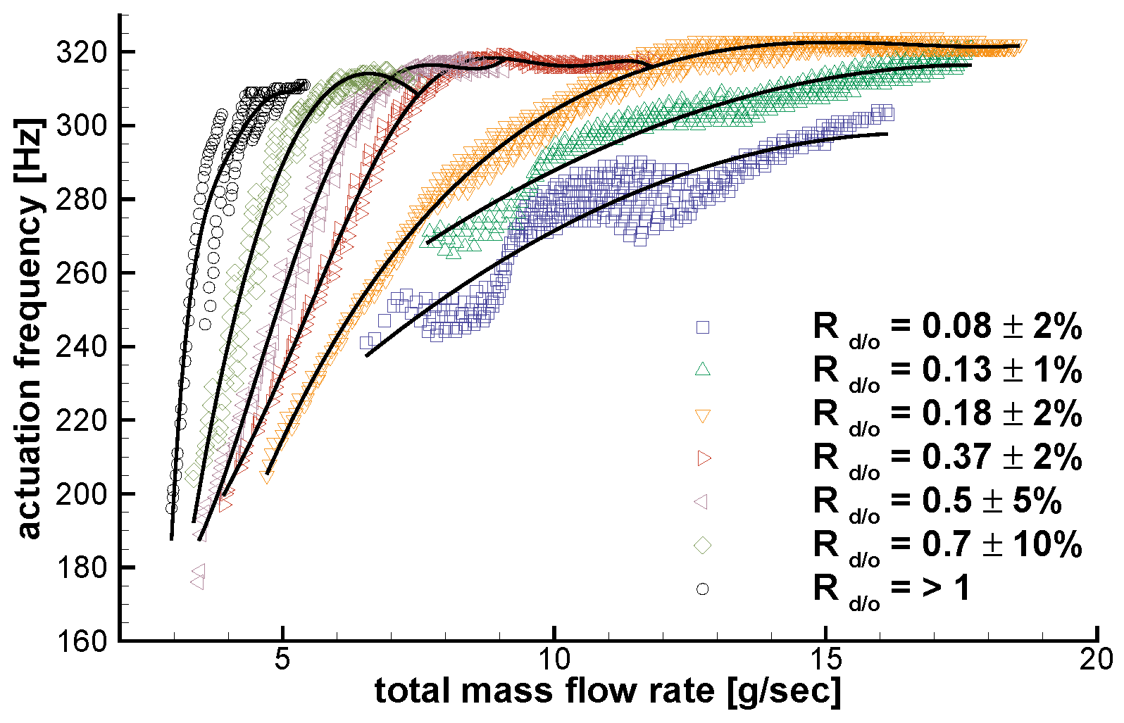
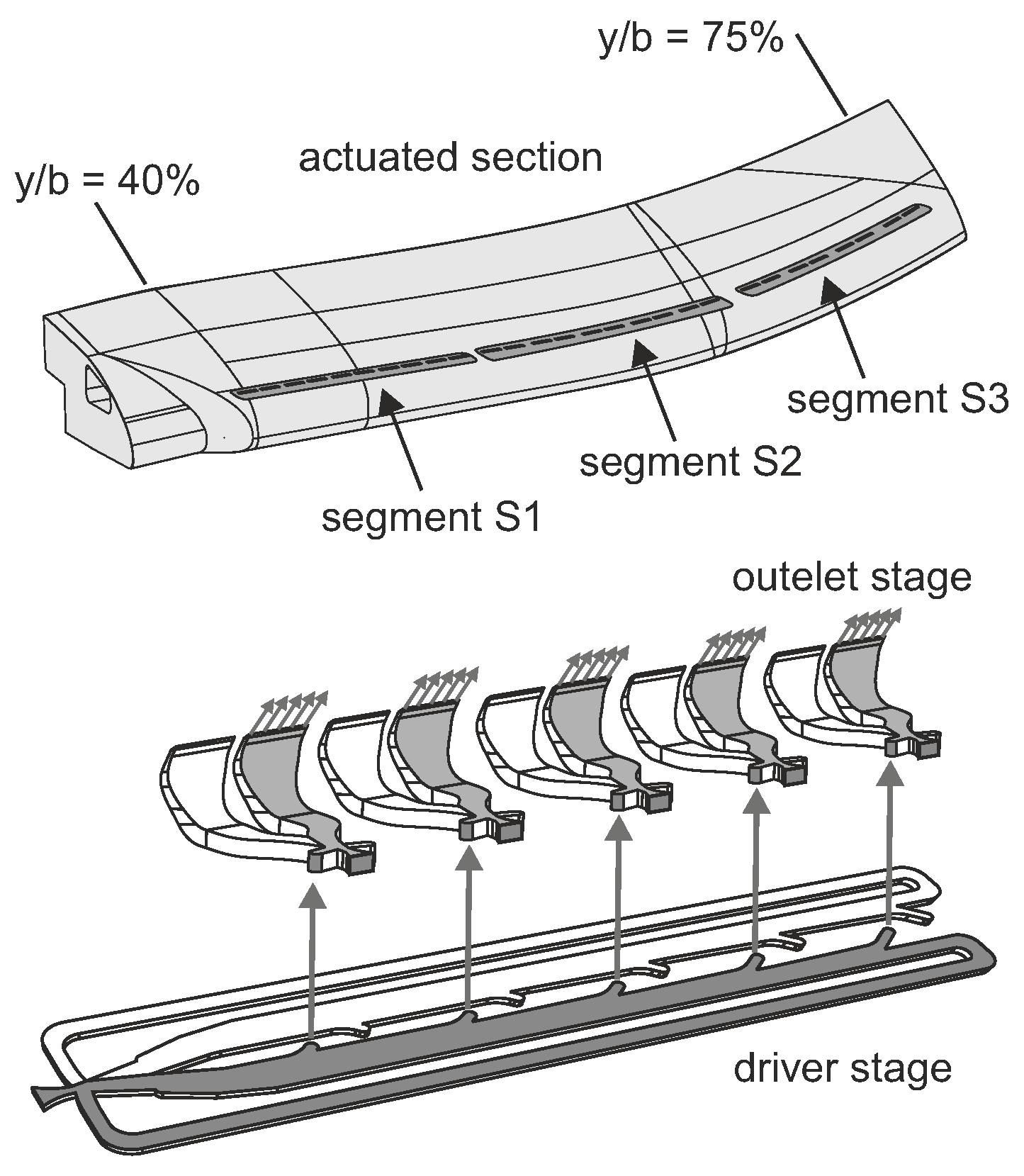
The results for the controlled flow are presented in this section. The performance of AFC will be quantified in terms of the gain in the maximum lift, reduction in drag compared to the base flow at $\alpha \left(C_{L,max,AFC}\right)$ and offset of the stall angle. A deeper understanding of the changes in the flow field is gained by analyzing wake measurements conducted with a traversable five-hole probe rake. Finally, the efficiency of this AFC approach is evaluated in terms of the first aerodynamic figure of merit. In addition to the momentum coefficient, the jet velocity ratios $VR=u_{jet,peak}/u_{\infty }$ are quoted in the figure legend in order from inboard (S1) to outboard (S3), i.e., ($V{R}_{S1}$, $V{R}_{S2}$, $V{R}_{S3}$). Although previous experiments on a similar geometry have shown no significant impact of the actuation frequency on the control results, an attempt was made to keep the forcing frequency constant across the actuation amplitude range tested. The frequency band for Segments S1 and S2 ranges from $F_{min}^{+}=2.06$ (295 Hz) for $VR=2.0$ to $F_{max}^{+}=2.2$ (315 Hz) for $VR=4.5$. Geometric constraints required a shorter feedback structure on Segment S3, resulting in a higher frequency band, which ranges from $F_{min}^{+}=2.66$ (380 Hz) for $VR=2.0$ to $F_{max}^{+}=2.85$ (407 Hz) for $VR=4.8$.

3.3.1. Global Effects of Flow Control

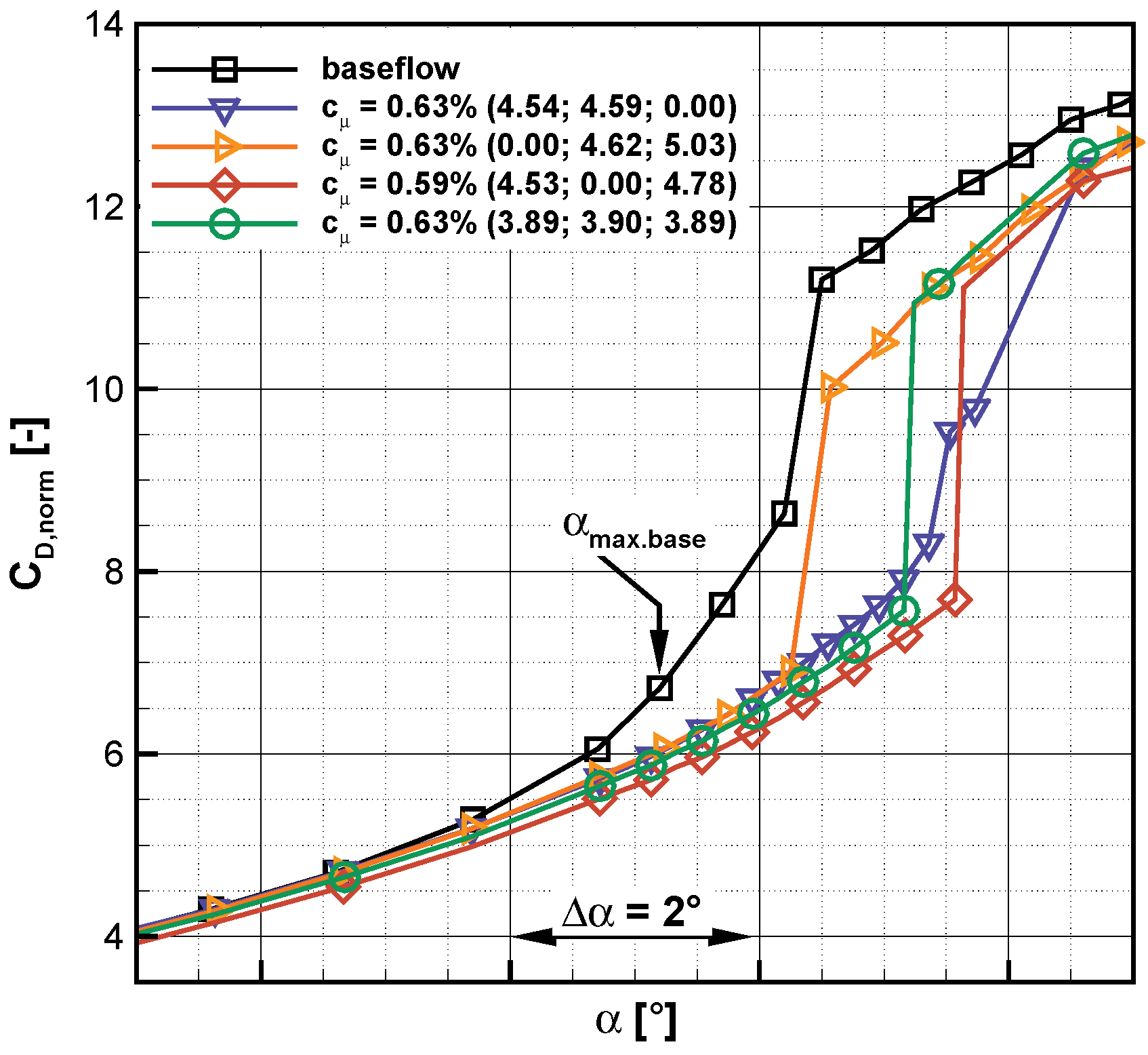
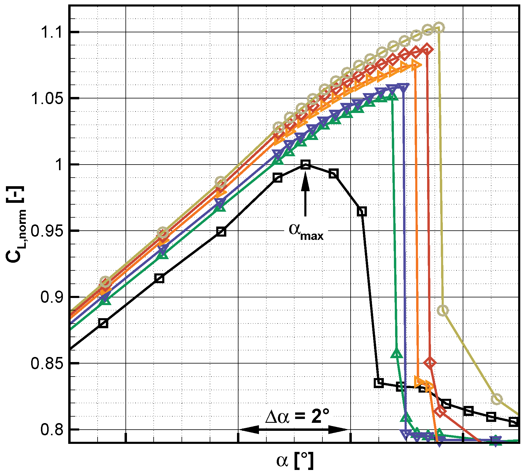
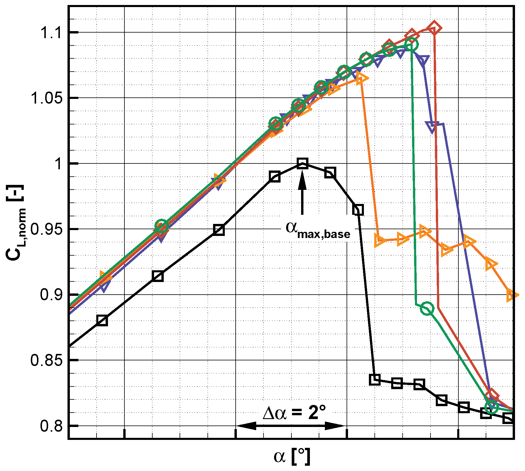
In previous experiments on a similar geometry, we observed that the flow control effectiveness was sensitive to the distribution of actuation along the span. Therefore, the effect of different combinations of segment-wise actuation was evaluated for a constant overall forcing amplitude of $c_{\mu }\approx 0.6\%$. The resulting drag and lift coefficient curves are presented in Figure 11 and Figure 12, respectively.

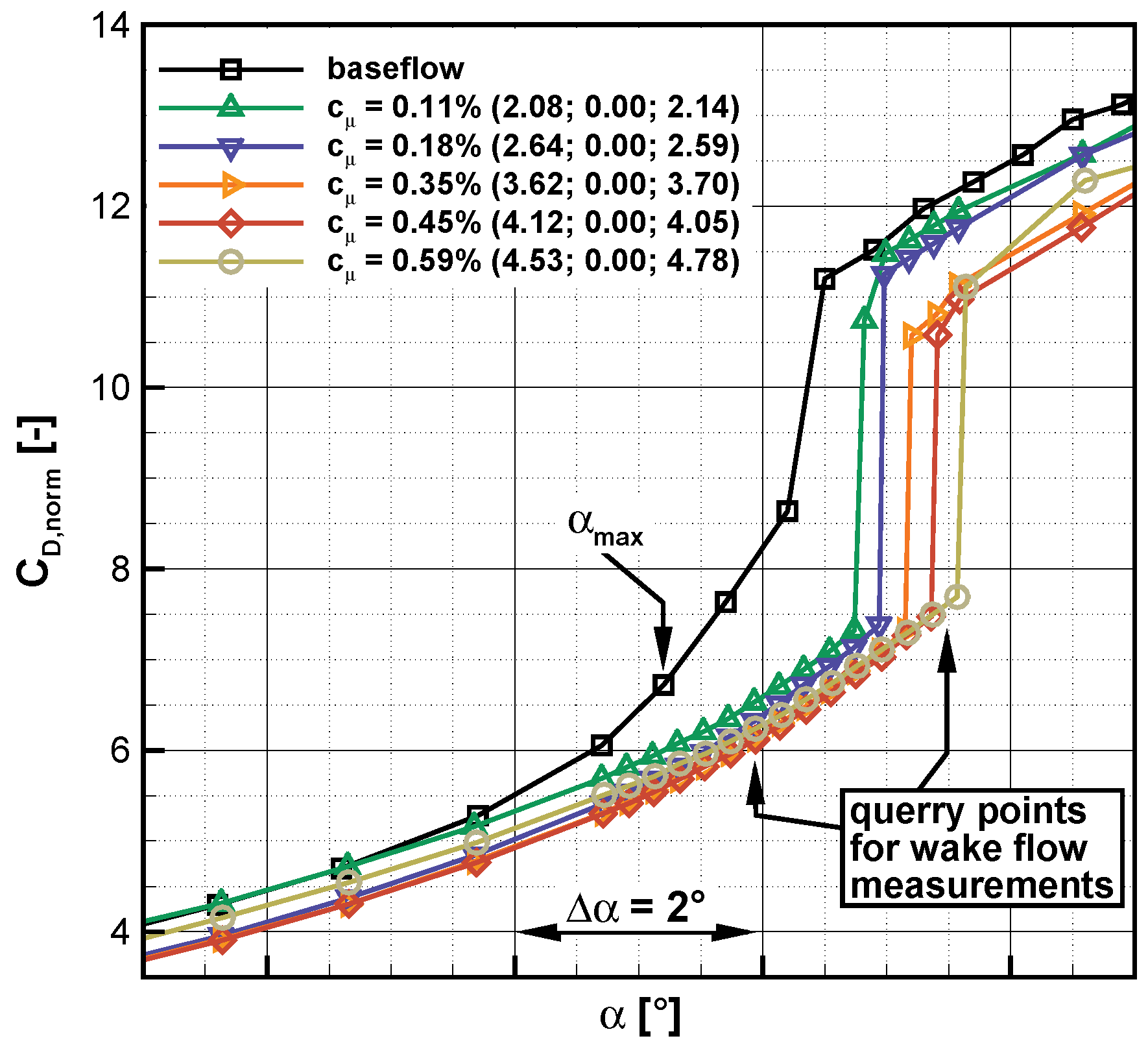
All of the combinations tested improved the stall behavior of the model wing. Although the extent of the improvement differs, the underlying trends are similar. At a sufficiently low incidence (e.g., ${\alpha }_{max}$−4°), the effect of flow control on the drag coefficient is negligibly small. In the incidence range between ${\alpha }_{max,base}$−3° and the corresponding ${\alpha }_{max,AFC}$, the (ideally) parabolic shape of the drag coefficient curve is maintained as a result of forcing. This can be attributed to the reduction in the cross-flow on the model and the prevention of separation on the outboard half of the wing. In contrast to the drag, the lift is affected by flow control over the entire range of the angles of attack tested. In the linear range of the lift curve, the lift coefficient is offset by a constant $\mathrm{\Delta }{C}_L$ depending on the momentum coefficient, but not on the distribution of the actuation along the span. Once stall occurs, the resulting drag rise and lift drop are more abrupt than those for the base flow. Here, the exception is actuation with Segments S1 and S2 combined, for which separation on the model occurs in two distinct steps. For this combination, the flow on the winglet separates, but the flow stays attached in the region trailing the slat edge for an additional $\mathrm{\Delta }\alpha =0.4^{°}$. This results in an intermediate step in the drag coefficient curve and milder stall behavior.

The difference in effectiveness for the segment combinations tested becomes apparent when the stall angle (${\alpha }_{max,AFC}$), maximum lift ($C_{L,max,AFC}$) and drag coefficient value ($C_D$) at each ${\alpha }_{max,AFC}$ are considered. According to those indicators, actuation with Segments S1 and S3 yields the highest benefit. For a momentum coefficient of $c_{\mu }=0.6\%$, forcing with these two segments offsets stall by 2.4° and increases the maximum lift coefficient by more than 10%. The drag coefficient at ${\alpha }_{max,AFC,S1\&S3}$ is reduced by 37% with respect to the base flow value.

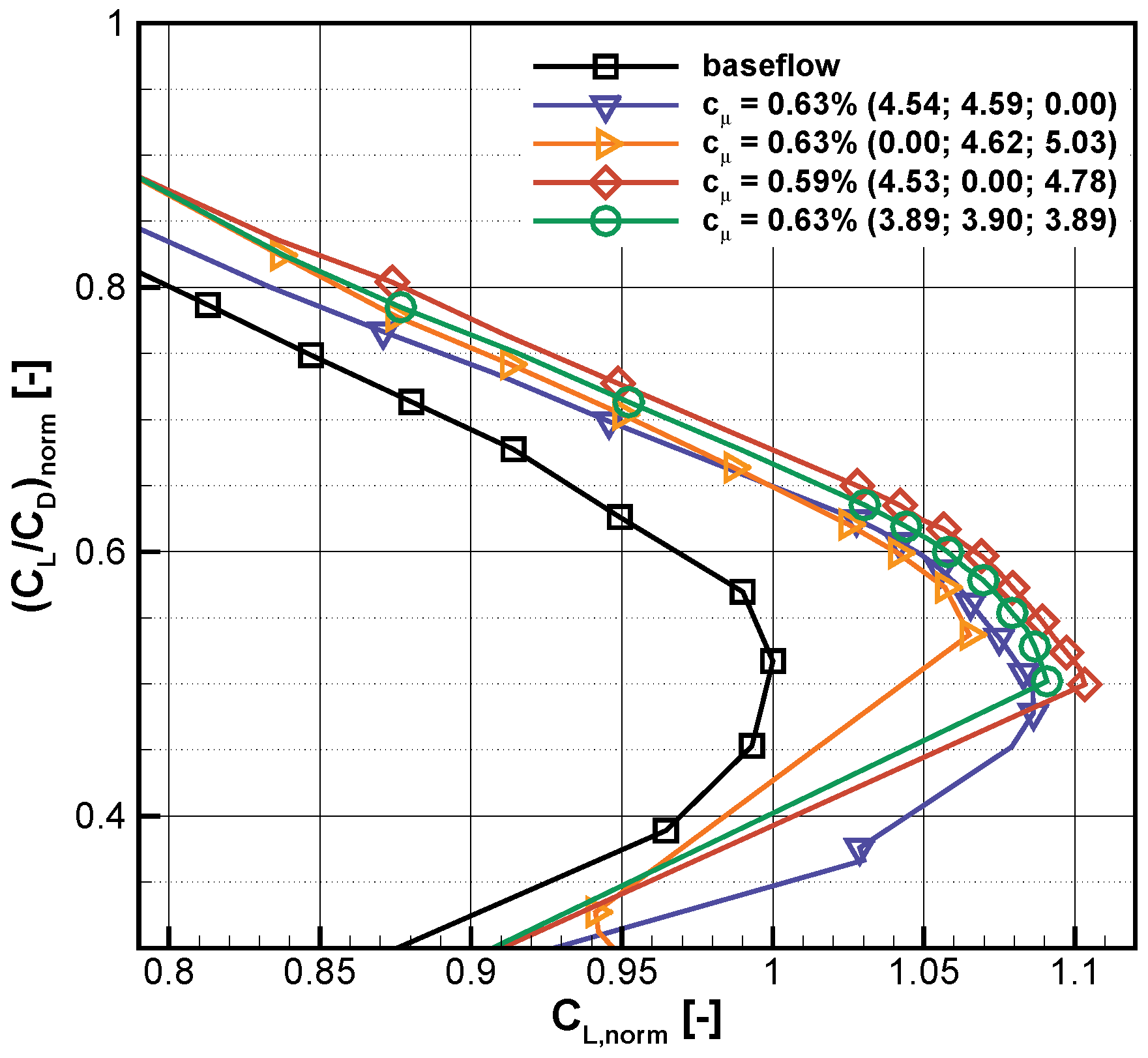
The aerodynamic efficiency of a wing is given by the ratio of $C_L$ over $C_D$, which is plotted versus the lift coefficient in Figure 13 for the segment variation considered above. Again, with respect to this quantity, the combination of Segments S1 and S3 produces the best results. The effect of flow control is positive over the entire incidence range. At the original (base flow) $C_{L,max,base}$, the aerodynamic efficiency is increased by 30%, whereas for maintaining the original aerodynamic efficiency, a lift increase of 9.5% is achievable. Actuation with all other combinations of segments is beneficial as well, but to a lesser extent.

For actuation using the most effective segment combination, Segments S1 and S3, the drag and lift coefficient curves for different forcing amplitudes are presented in Figure 14 and Figure 15, respectively. Increasing the forcing amplitude successively improves the aerodynamic performance of the model wing, and no saturation is observed within the available range of momentum coefficients. The highest forcing amplitude of $c_{\mu }=0.59\%$ is produced at a jet velocity ratio of approximately 4.7, which implies an almost sonic peak jet exit velocity ($M{a}_{jet,peak}\approx 0.95$). Between the lowest ($c_{\mu }=0.11\%$) and highest ($c_{\mu }=0.59\%$) forcing amplitudes tested, the resulting offset in stall angle ranges from $1.5^{°}<\mathrm{\Delta }{\alpha }_{max,AFC}<2.4^{°}$, and the maximum lift increases in the range of $5\%<\mathrm{\Delta }{C}_{L,max,AFC}<10.4\%$. The drag reduction at ${\alpha }_{max,AFC}$ varies only slightly within the band of forcing amplitudes tested, showing an improvement of approximately $37\%$ compared to the uncontrolled base flow.

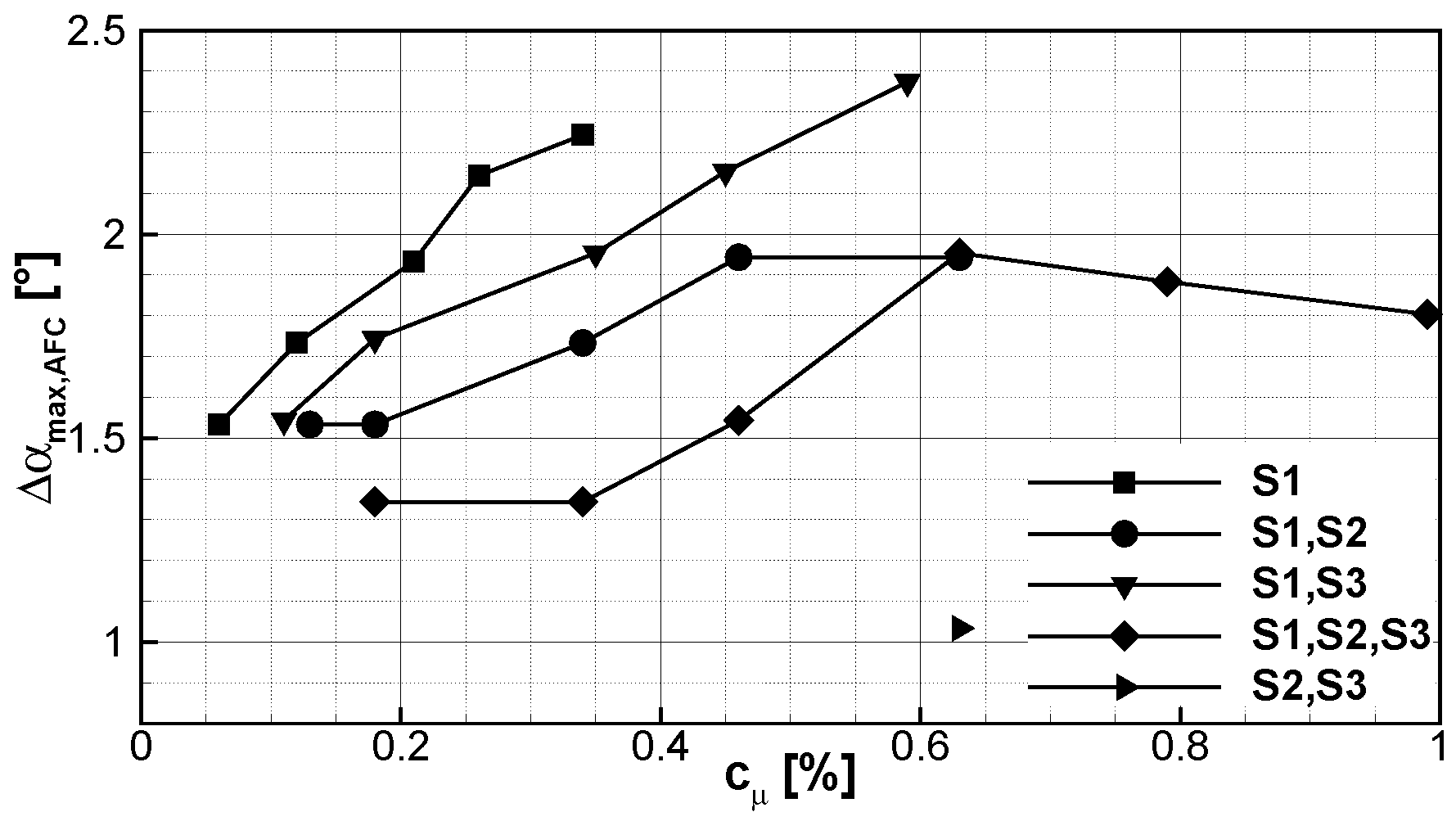
An overview of the flow control performance as a function of the momentum coefficient and jet velocity ratio for different combinations of segments is provided in Figure 16, Figure 17, Figure 18 and Figure 19. Note that only one data point is available for the combination of Segments S2 and S3. The offset in the stall angle is presented in Figure 16 as a function of the momentum coefficient.

With respect to the stall angle, it is noteworthy that forcing with only Segment S1 significantly shifts the onset of stall to higher incidences at relatively low momentum coefficients, offsetting stall by up to $\approx 2.2^{°}$ at a momentum coefficient of $c_{\mu }=0.34\%$. In comparison, actuation with Segments S1 and S3 can produce a higher maximum shift in ${\alpha }_{max}$ (additional $\mathrm{\Delta }{\alpha }_{max}$ of $0.{25}^{°}$), but this combination requires almost twice the investment in terms of the momentum coefficient to produce an identical offset in the stall angle. All other combinations of segments increase the stall angle by less than 2°. 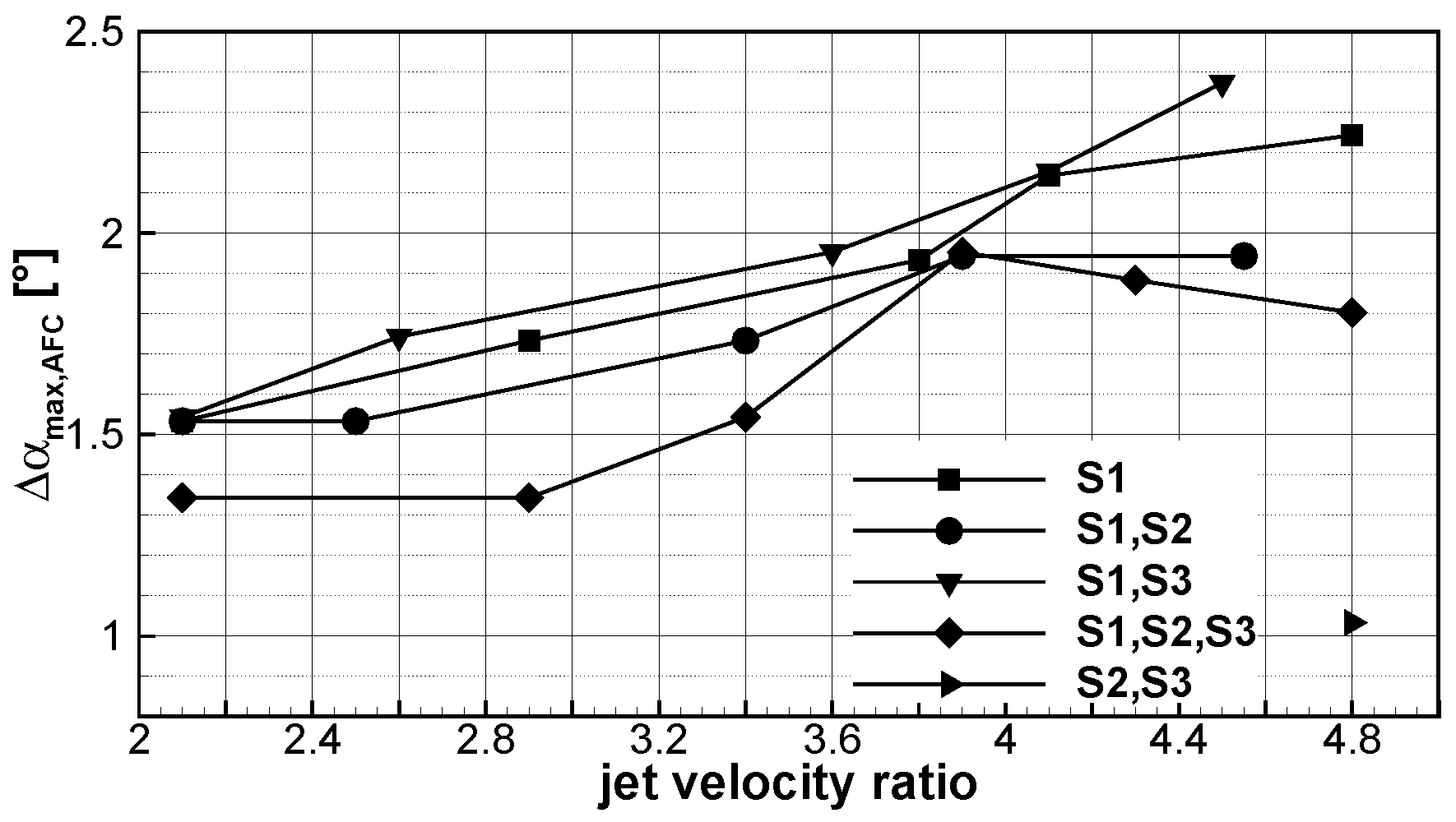Plotting $\mathrm{\Delta }{\alpha }_{max,AFC}$ versus the jet velocity ratio (see Figure 17) appears much better suited to collapse the curves shown, indicating that, with respect to the increase in the stall angle, this ratio is the dominant AFC parameter compared to the total momentum or mass addition. For velocity ratios smaller than four, the curves for the segment combinations (S1), (S1,S2) and (S1,S3) lie within a band of $\mathrm{\Delta }{\alpha }_{max,AFC}\pm 0.1^{°}$ from the average value. The results for forcing with all three segments (S1,S2,S3) lie below this band as a result of the different (two-step) stall behavior described above. For velocity ratios larger than four, the curves diverge, as forcing combinations that include segment S2 do not lead to additional benefit in terms of a further increase in jet exit velocity. 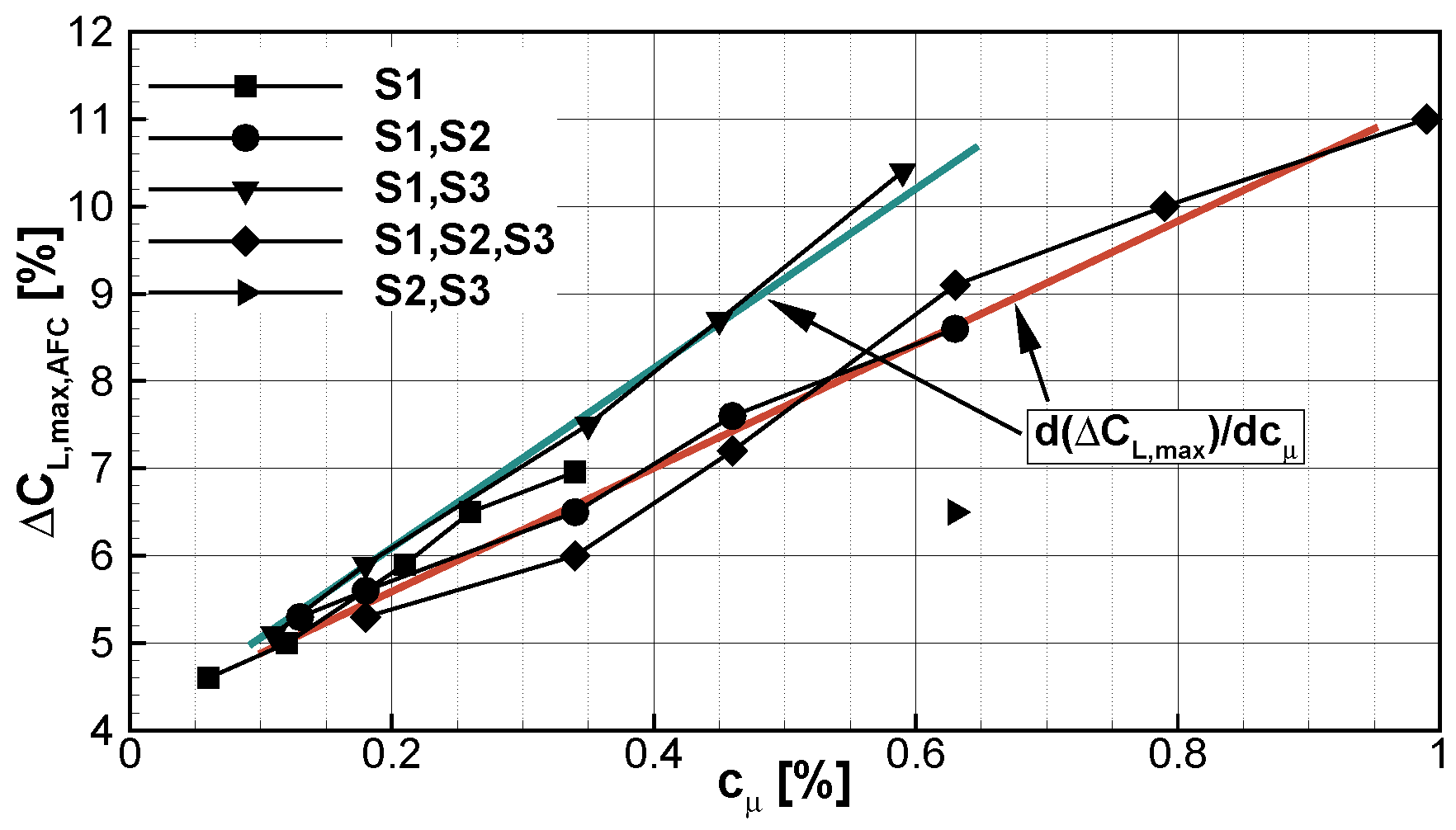The lift gain as a function of $c_{\mu }$ is presented in Figure 18.

Here, an almost linear increase in the lift gain is observed with increasing momentum coefficient. The slope ($d\left(\mathrm{\Delta }{C}_{L,max}\right)/d{c}_{\mu }$) of the curves associated with forcing with Segment S1 only and with Segments S1 and S3 combined is steeper than that for any segment combination that includes forcing with Segment S2. The inefficiency of including Segment S2 in the control attempt becomes apparent when actuation with Segments S1 and S3 is compared to actuation with all three segments. While the maximum increase in $C_{L,max,AFC}$ is marginally higher when all three segments are operated ($\mathrm{\Delta }{C}_{L,max,S1\&S2\&S3}$ = 11% vs. 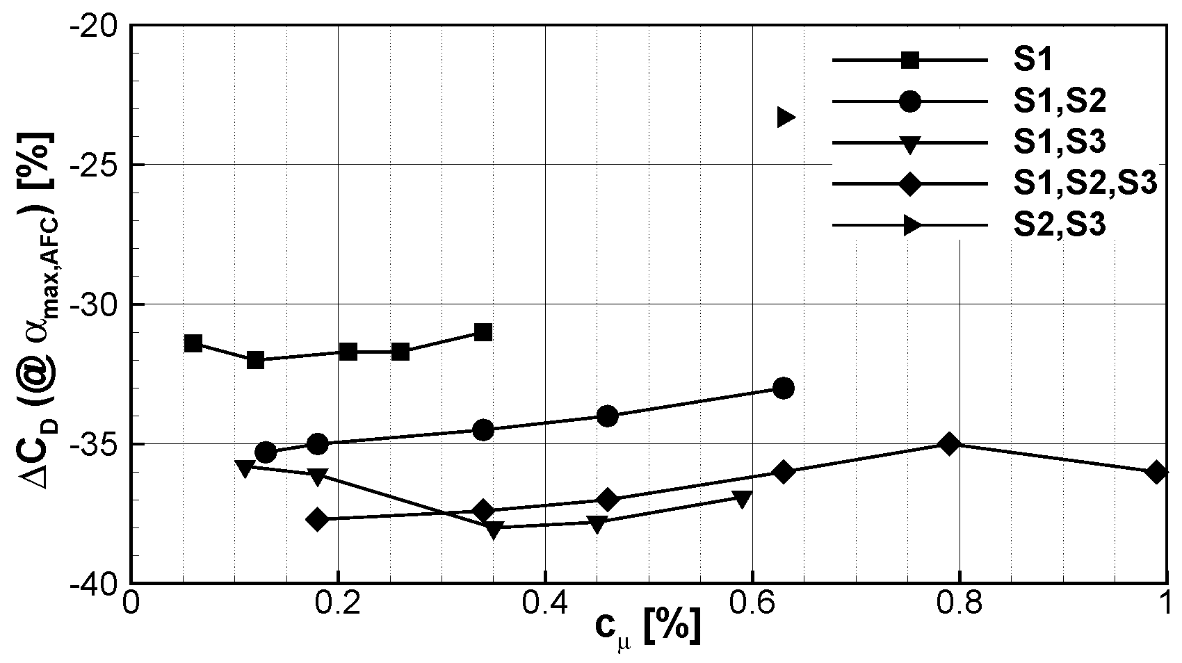$\mathrm{\Delta }{C}_{L,max,S1\&S3}$ = 10.4%), the required momentum input in terms of momentum coefficient to achieve a similar lift gain is approximately 40% higher than for actuation with Segments S1 and S3 only. Although the offsets in the stall angle and lift gain exhibit a distinct dependence on the momentum coefficient, this is not observed in the reduction of the drag at ${\alpha }_{max,AFC}$ relative to the respective base flow values, as shown in Figure 19.

Here, the percentage by which the drag coefficient is reduced is approximately constant across the range of momentum coefficients tested and depends only on the combination of segments operated. The highest drag reduction is realized using the combination of Segments S1 and S3 or Segments S1, S2 and S3, which decreases the drag coefficient by approximately 37%. Operation of Segments S2 and S3 yields the least benefit, resulting in a drag decrease of less than 23%.

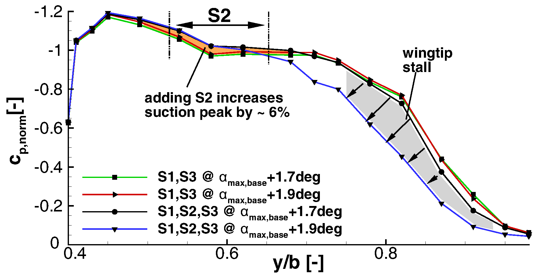
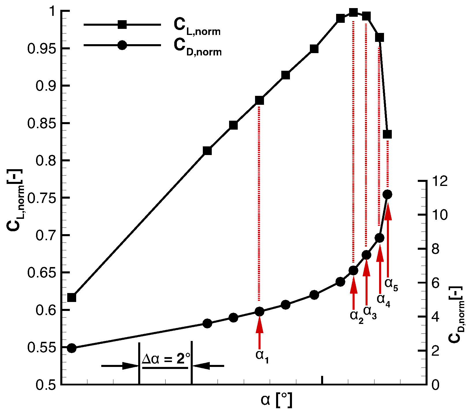
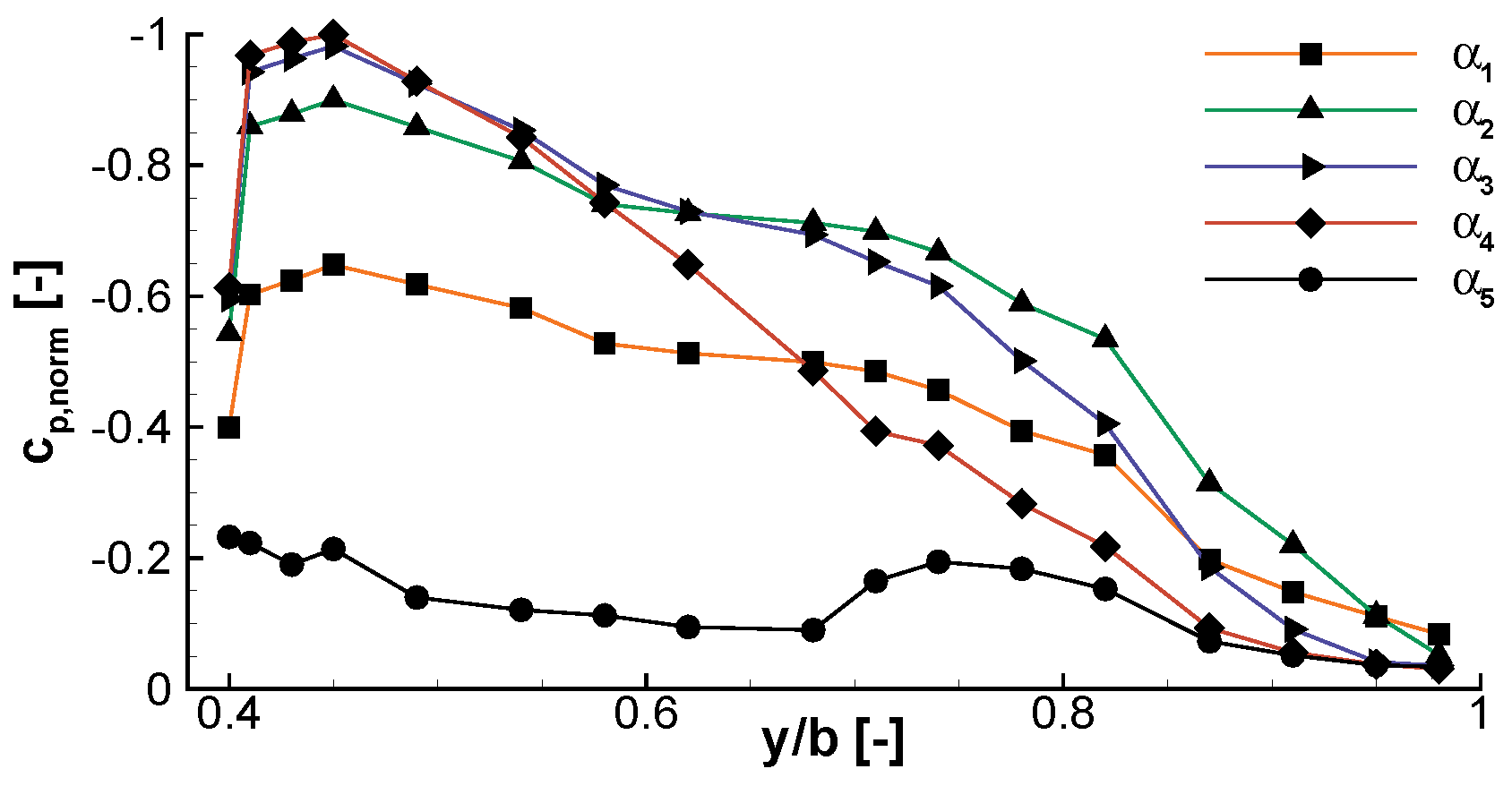
To conclude this section on the global effects of flow control, we attempt to explain the counterintuitive observation that the addition of local forcing (namely with Segment S2) deteriorates the effectiveness of AFC for otherwise identical forcing parameters. For this purpose, the pressure coefficient distribution along the span (constant $x/c$ = 0%) is displayed in Figure 20 for two different combinations of segments: inner and outer segments (S1, S3; $c_{\mu }=0.59\%$) and all three segments (S1, S2, S3; $c_{\mu }=0.79\%$), with all segments operated at a velocity ratio of $u_{jet,peak}/u_{\infty }\approx 4.5$. The incidence angles shown correspond to ${\alpha }_{max,AFC,S1\&S2\&S3}$ (which is 1.7° beyond ${\alpha }_{max,base}$) and an additional increment of +0.2°.

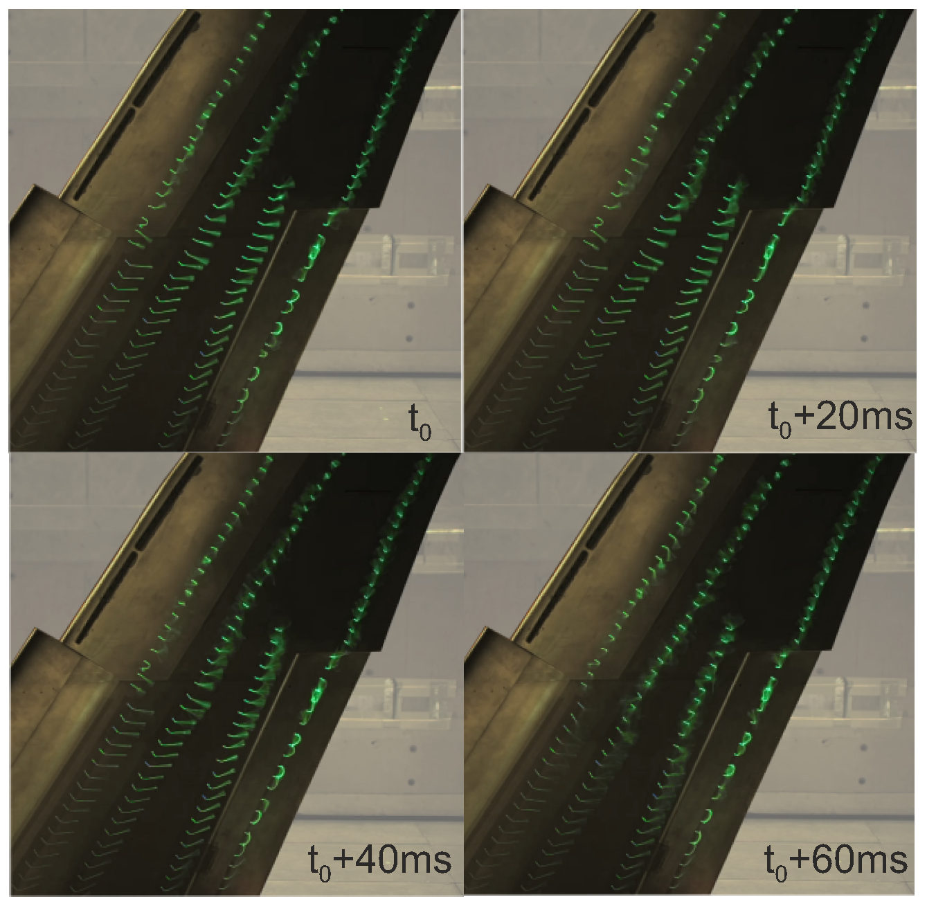
Near the active Segment S2 (as marked in the figure), we find that the suction peak is 6% larger than when S2 is inactive. This favorably affects the lift coefficient at lower angles of attack. However, the reduced pressure in this region causes increased aerodynamic loading on the model wing in this area, making it more prone to separation. Additionally, this low pressure region causes the jets emanating from the outboard Segment S3 to be attracted into this region, directing their effect away from the wing tip, where, as a consequence, separation occurs earlier. This observation is confirmed in tuft flow visualization (data not shown).

3.3.2. Effect of AFC on Model Wake Flow

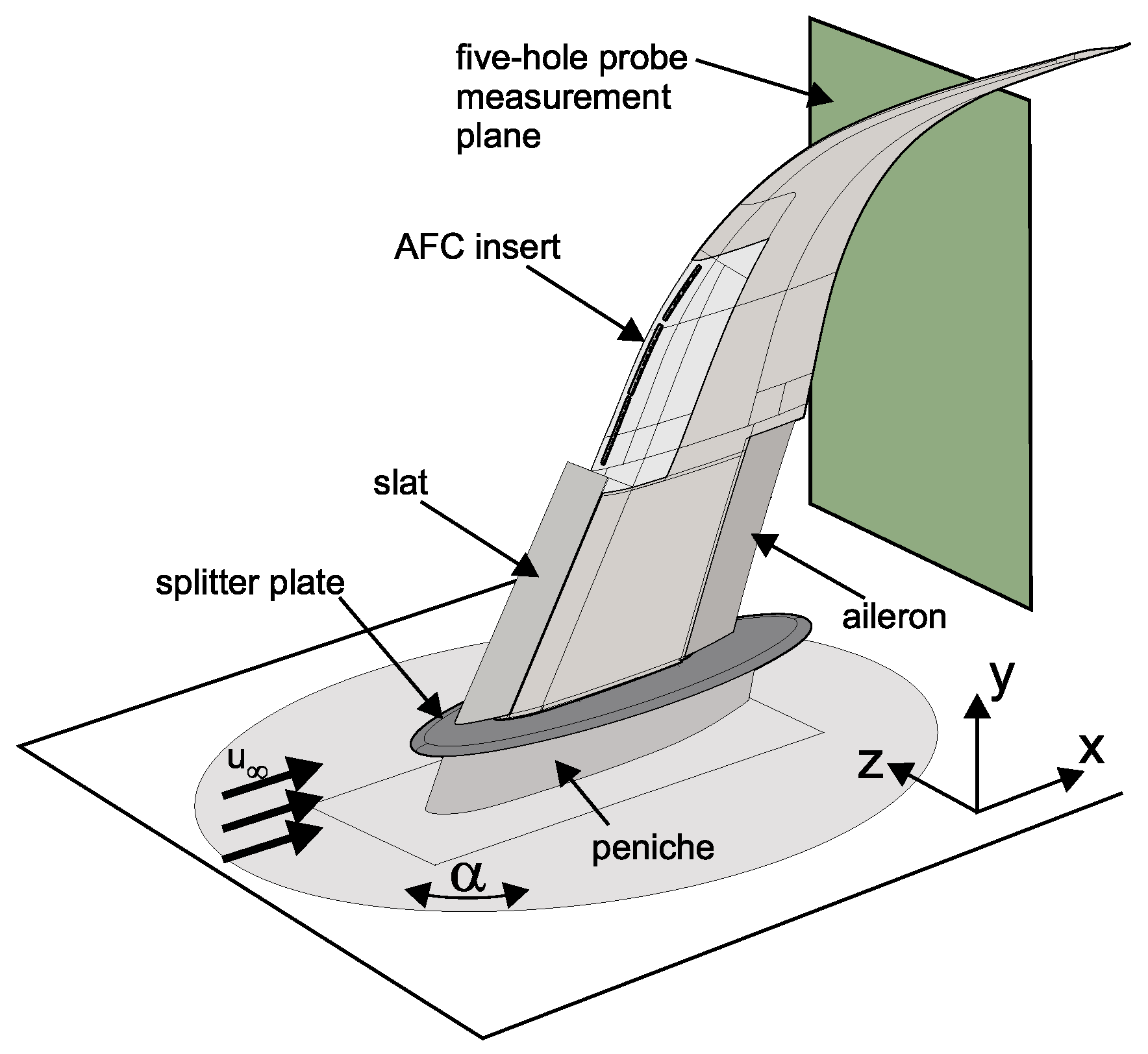
A traversable five-hole probe rake was used to quantify the effect of flow control on the wake flow of the outer wing model to gain insight into how the changes are spatially distributed in the flow field. The flow conditions for two incidence angles (marked in Figure 14) are evaluated. The plots show the Mach number (normalized by the incidence Mach number) measured in the plane of the rake together with the vectors for the velocity components in the y and z directions observed from a downstream position looking upstream.

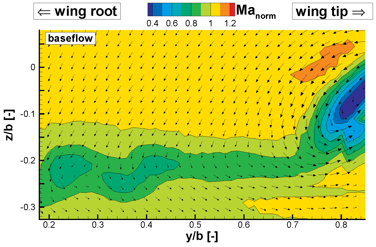
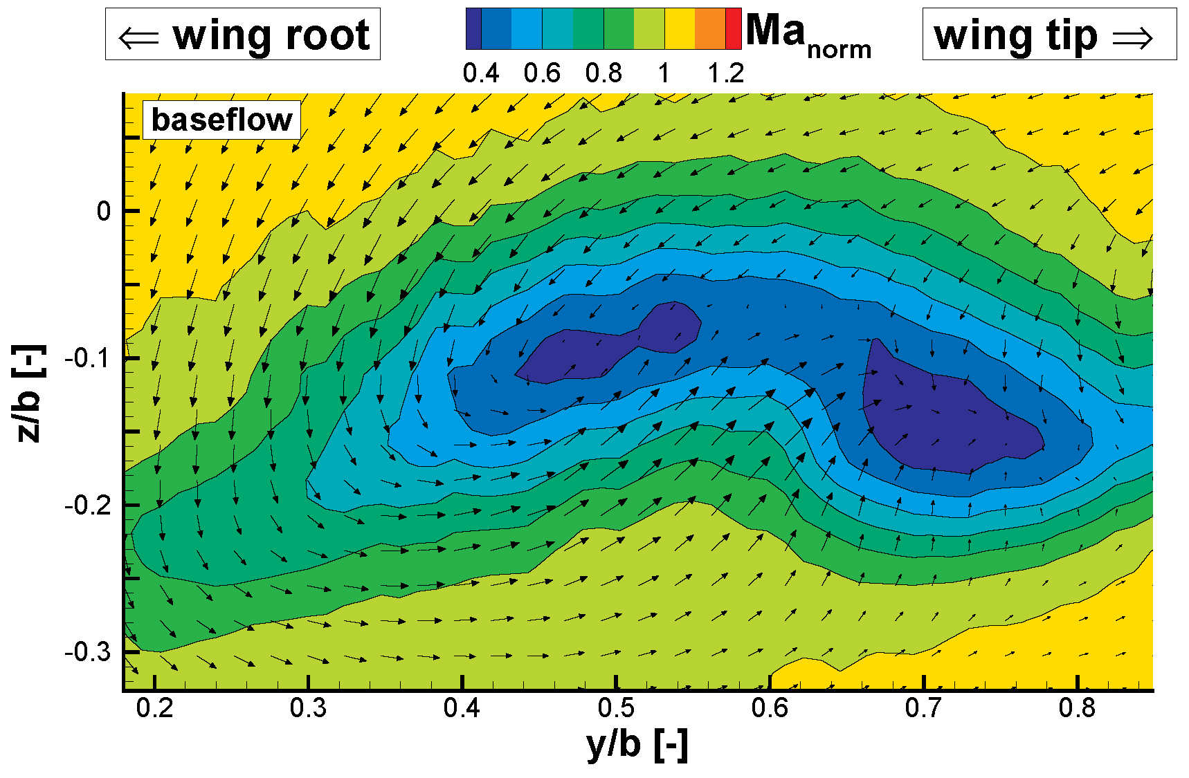
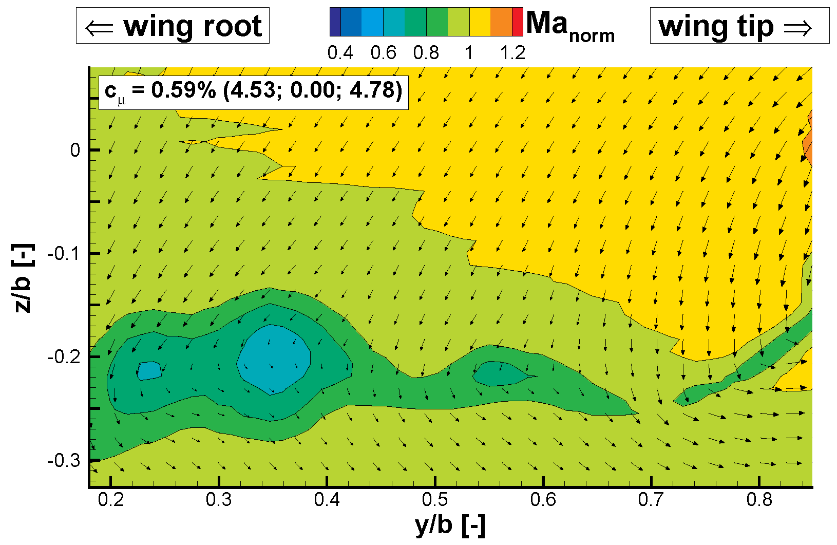
First, the data for an angle of attack of (${\alpha }_{max,base}+0.7^{°}$) are presented, at which a significant drag reduction of more than 20% is noted, although the baseline flow is not fully separated yet. The results for the uncontrolled flow are shown in Figure 21. Here, the most prominent feature is the large vortical structure formed at the wing tip by flow separation. It manifests as a region of low velocity, highly rotational flow motion in the wake field and low static pressure (pressure data not shown) at its center. Flow control can completely suppress the separation on the wing tip, as is apparent from Figure 22. The velocity losses associated with the onset of trailing edge separation on the entire span are reduced, and the slat edge vortex (at $y/b\approx 0.35$) is more defined in the case of controlled flow. Note that the magnitude of the cross-flow component directed outward (positive y direction) is also reduced when forcing is applied. A second set of data is presented for an incidence close to the maximum angle of attack of the controlled flow (${\alpha }_{max,AFC,S1\&S3}\approx {\alpha }_{max,base}+2.3^{°}$). For the base flow (see Figure 23), a massive separation is observed downstream of the model where no slat is installed, accompanied by extensive velocity losses (down to 30% of the incidence velocity). The downwash normally produced by the lifting surface is replaced in parts by upwash, reflecting the shedding of vortices at the leading and trailing edges of the wing model.

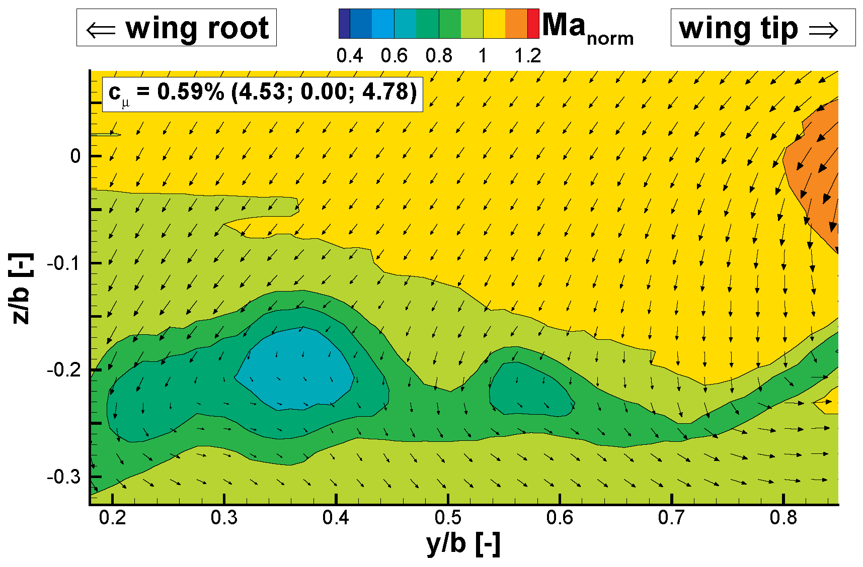
In comparison, the wake flow measurements for the controlled flow, shown in Figure 24, illustrate the ability of AFC to stabilize the flow on the wing and to suppress separation completely. The large region of high velocity losses is reduced to the size commonly found downstream of the trailing edge of a wing. Now, the highest magnitude of the velocity deficit is found in the center of the slat edge vortex and its associated secondary vortex (at $y/b\approx 0.35\%$) and downstream of the location of (inactive) Segment S2. It is noteworthy that the (controlled) flow structure at this high angle of attack closely resembles that shown at lower incidence angles, differing mainly in the size of the slat-edge-induced velocity deficit, although the wing is very close to stall.

3.3.3. Consideration of Flow Control Efficiency

To conclude the analysis of the effect of flow control on the aerodynamic performance, we focus on the efficiency of our flow control approach. To quantify this, we employ the first aerodynamic figure of merit (AFM1), as introduced by Seifert [20]. It is defined as:

$$AFM1=\frac{{\displaystyle \frac{u_{\infty }L}{(u_{\infty }D+P_{AFC})}}}{{\displaystyle {(L/D)}_{baseline}}}$$

(1)

L and D are the integral (balance-measured) values of the lift and drag, respectively, and $P_{AFC}$ refers to the actuator power consumption. The ratio in the denominator with subscript baseline is the value for the uncontrolled flow. The jet power $P_{jet}$ of the AFC system is calculated, under the same assumptions as those for the calculation of the momentum coefficient, from the peak jet velocity and measured mass flow rate. This value is modified by a loss factor ${\xi }_{AFC}$ that describes the actuator internal energy conversion efficiency to yield the flow control system power consumption $P_{AFC}=P_{jet}/{\xi }_{AFC}$. To portray the efficiency of a more realistic actuator system, the value for the loss factor is estimated to be ${\xi }_{AFC}=0.5$, which is considered to be a conservative assumption based on previous work with this type of actuator system as reported in, e.g., [21]. The actual energy supplied to the model AFC system was not recorded, as this value would not be representative owing to the design compromises necessary to fit the actuators into the model at wind tunnel scale (note that for the data shown, an energy conversion efficiency of approximately 3% would still produce $AFM1$ values greater than unity).

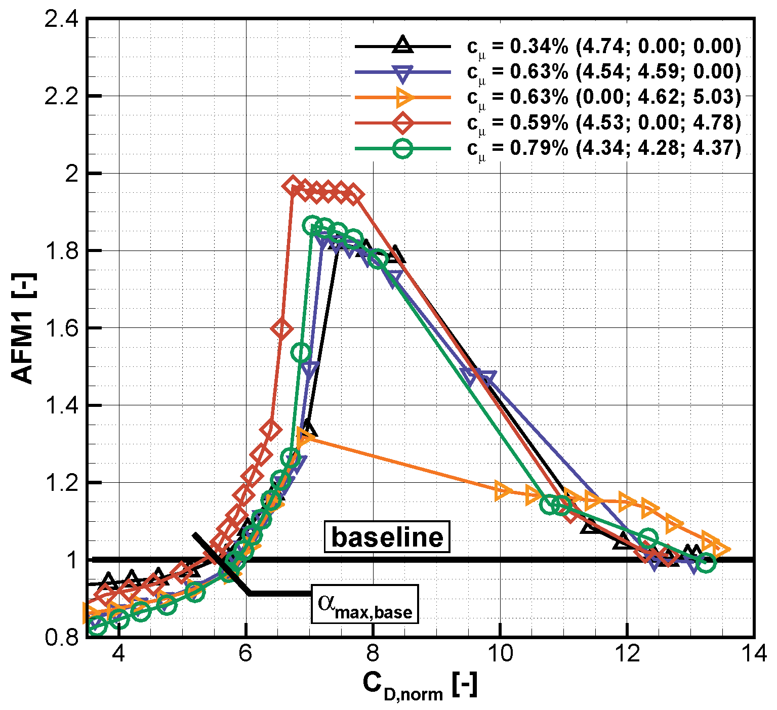
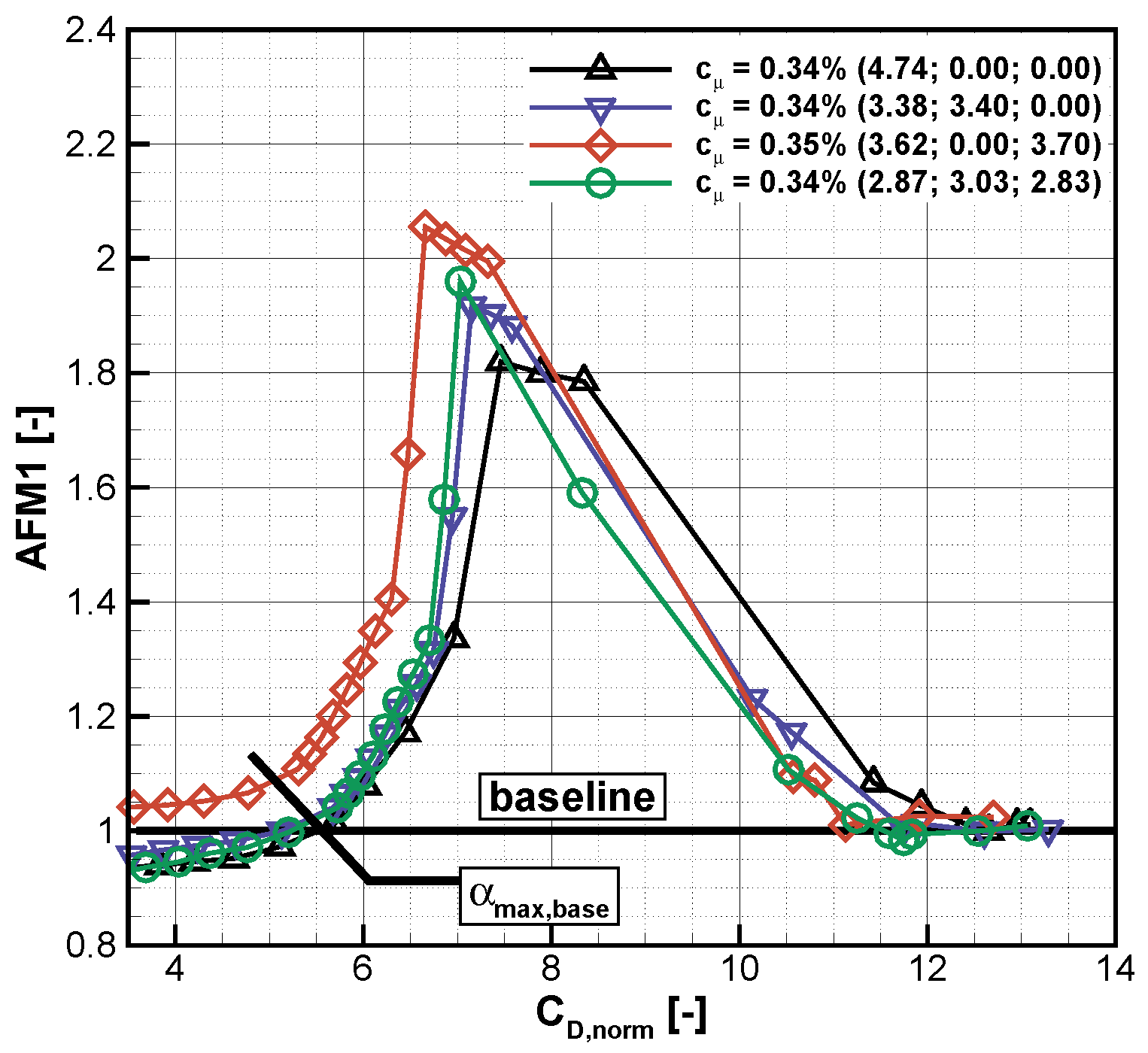
The $AFM1$ value for different segment combinations is plotted in Figure 25 for a constant jet velocity ratio of $u_{jet}/u_{\infty }\approx 4.4$ and in Figure 26 for a constant total momentum coefficient of $c_{\mu }\approx 0.34\%$. $AFM1$ values larger than unity reflect efficient use of the energy supplied. Three distinct regimes can be identified. For low drag coefficient values, which correspond to low angles of attack, the flow is attached naturally to the wing, and the lift increase produced at those incidences does not warrant the efficient use of flow control, as indicated by $AFM1$ values smaller than unity. At incidence angles where the flow is kept attached only because of flow control, all of the combinations of segments tested produce $AFM1$ values larger than unity. The peak values, however, depend largely on the combination of segments chosen. For a similar momentum coefficient and jet velocity ratio, forcing with Segments S2 and S3 combined yields $AFM1\approx 1.3$, whereas the combination of Segments S1 and S3 combined produces $AFM1\approx 1.95$. A comparison of the curves for the combination of S1 and S3 in Figure 25 and Figure 26 shows that lowering the forcing amplitude to a certain degree increases the $AFM1$ value ($AFM1(c_{\mu }=0.59\%)\approx 1.95$ ⇒ $AFM1(c_{\mu }=0.35\%)\approx 2.05$), indicating a more efficient use of energy, but the effectiveness is reduced. Once the flow separates from the wing, despite the attempt at flow control, the $AFM1$ values drop to approximately unity.

4. Conclusions

AFC by means of pulsed air jet blowing was applied to a realistic outer wing model to counter performance degradation at high angles of attack. The experiments were conducted at the nominal take-off incidence Mach number of $M=0.2$. Although all of the forcing parameter variations tested improve the aerodynamic performance, the results reveal that the control effect is highly sensitive to the local distribution of momentum and mass introduction. The most effective set of forcing parameters, actuation with Segments S1 and S3 combined using a momentum coefficient of $c_{\mu }=0.59\%$, offsets the stall angle by 2.4°, increases the maximum lift by 10.5% and decreases the drag at ${\alpha }_{max,AFC}$ by 37%. The application of flow control was found to change the stall behavior of the model wing. As the base flow separates gradually from the wing, with separation progressing from outboard to inboard with increasing incidence, stall occurs abruptly on the entire model under controlled flow. The actuation efficiency, measured in terms of the first aerodynamic figure of merit, improves significantly if the actuation effort is distributed advantageously along the span. Further improvement of efficiency might be gained by increasing the spacing between adjacent actuator outlets. This geometry parameter was fixed during these experiments and was not tested for optimality so far. However, if it is possible to increase the spacing without compromising effectivity, doing so would contribute directly to lowering $c_{\mu }$ and to reducing the required mass flow rate.