Climate-Compatible Air Transport System—Climate Impact Mitigation Potential for Actual and Future Aircraft

Abstract

Aviation guarantees mobility, but its emissions also contribute considerably to climate change. Therefore, climate impact mitigation strategies have to be developed based on comprehensive assessments of the different impacting factors. We quantify the climate impact mitigation potential and related costs resulting from changes in aircraft operations and design using a multi-disciplinary model workflow. We first analyze the climate impact mitigation potential and cash operating cost changes of altered cruise altitudes and speeds for all flights globally operated by the Airbus A330-200 fleet in the year 2006. We find that this globally can lead to a 42% reduction in temperature response at a 10% cash operating cost increase. Based on this analysis, new design criteria are derived for future aircraft that are optimized for cruise conditions with reduced climate impact. The newly-optimized aircraft is re-assessed with the developed model workflow. We obtain additional climate mitigation potential with small to moderate cash operating cost changes due to the aircraft design changes of, e.g., a 32% and 54% temperature response reduction for a 0% and 10% cash operating cost increase. Hence, replacing the entire A330-200 fleet by this redesigned aircraft ($M{a}_{cr}$ = 0.72 and initial cruise altitude (ICA) = 8000 m) could reduce the climate impact by 32% without an increase of cash operating cost.

1. Introduction

The environmental impact of aviation, in terms of gaseous pollutants and noise emissions, becomes more and more important to society. Aviation emissions alter the radiative characteristics of the Earth-atmosphere system and lead to an increase of global surface temperature. Aviation was assessed to account for a total radiative forcing (RF) of 78 mW·m${}^{-2}$ (38–139 mW·m${}^{-2}$, 90% likelihood range) in 2005, including the impact from aviation-induced cirrus clouds [1].

Commercial aviation has experienced a steady growth of travel rates over the last decades and is expected to grow approximately 4.6% per year in terms of passenger kilometers in the next 20 years without further political measures [2]. This will largely surpass the typical annual fuel efficiency improvements of 1%–2% [2]. Along with this development, continuous improvements in transport efficiency also were achieved. However, despite these technological advances the growing demand of commercial air transport and the related number of conducted flights led to an increase in emissions and considerable changes of greenhouse gases, aerosols and induced cloudiness.

The rise of annual emission rates and induced cloudiness will hence further increase the climate impact from aviation. The Advisory Council for Aeronautical Research in Europe (ACARE) states, in this sense, that a socially- and climate-compatible air transportation system is required for a sustainable development of commercial aviation. Therefore, climate impact mitigation strategies have to be developed based on comprehensive assessments of the different impacting factors and reduction potentials.

In the past, a couple of mitigation strategies were analyzed. Many of them focus on a change in flight altitude to reduce the impact of contrails (e.g., [3,4,5,6,7]); others include additional effects, such as the climate impact from nitrogen oxide emissions (NO${}_{\mathrm{x}}$) (e.g., [8,9,10]). These studies have a focus on the climate impact, but apply simplified assumptions for aircraft performance. In addition, there are several studies that focus on aircraft design, but use simplified assumptions for the climate impact assessment (e.g., [11,12,13]).

The systematic assessment of aviation climate impact and the identification of the most suitable mitigation strategies represents a very challenging task. The atmospheric response to anthropogenic perturbations involves complex interdependent processes of very different natures acting on different spatial and temporal scales. The global climate impact from air traffic varies not only with the amount and type of emitted species, but also with altitude, location (longitude and latitude), time of day and season and atmospheric conditions. Further, changes in current flight procedures and aircraft design are likely to propagate to other areas of air traffic, which might provoke penalties for certain system stakeholders. Although environmental sustainability becomes increasingly important for society, current air traffic is so far purely cost driven. In this sense, nowadays, aircraft are designed for minimum operating costs: the airline operates the aircraft such that the highest revenues at the lowest possible costs are achieved, and the passenger dominantly chooses his/her flight according the lowest ticket price or best travel comfort. Changes towards improved climate impact of air traffic will often lead to cost penalties that have to be shared by the different stakeholders of the air transport system, those being the aircraft and engine manufacturers, airlines, air traffic management providers, regulatory authorities and not to forget the traveling passenger as customer. This, in turn, leads to a conflict between two basic expectations of society towards air traffic: the environmental sustainability vs. the price of air travel. It is hence essential to identify climate impact mitigation strategies with the best relation of benefit and costs.

The assessment of options to reduce the climate impact from aviation by operational and technological measures requires expert knowledge from different aviation disciplines and adequate models that sufficiently incorporate the driving impact factors. It further requires a comprehensive system analysis approach that integrates the relevant interdependencies for the development of cost-efficient mitigation strategies.

Such a comprehensive approach was developed within the DLR (Deutsches Zentrum für Luft- und Raumfahrt, German Aerospace Center) project CATS (Climate-compatible Air Transport System, 2008–2012). In this study, a summary of the project results is presented. A detailed description of the approach and results is given in Koch [14]. First, we quantify the climate impact mitigation potential and related cost penalty for current aircraft that are operated at different cruise altitudes and speeds. Further, we analyze the additional climate impact mitigation potential and cost improvement resulting from aircraft that are specifically designed for cruise conditions with reduced climate impact.

2. Climate Impact from Aviation

We will now describe the climate impact of aviation, mentioned in Section 1, in detail. The climate impact from air traffic results from induced cloudiness and concentration changes of atmospheric constituents caused by the emission of carbon dioxide (CO${}_2$), nitrogen oxides (NO${}_{\mathrm{x}}$), sulfur oxides (SO${}_{\mathrm{x}}$), water vapor (H${}_2$O) and aerosols [15]. These atmospheric perturbations change the terrestrial radiation balance and cause an RF that drives the Earth-atmosphere system to a new state of equilibrium through a resulting temperature change.

Table 1. Radiative forcing (RF) components from aviation effects in 2005 and 2010 (contrail-induced cloudiness (CiC)). Values and confidence intervals are taken from Lee et al. [1] and IPCC (Intergovernmental Panel of Climate Change) [16].

Confidence Intervals (mW·m${}^{-2}$)	CO${}_2$	O${}_3$	CH${}_4$	NO${}_{\mathbf{x}}$	H${}_2$O	SO${}_4$	Soot	CiC
Low	15.2	8.4	−2.4	3.8	0.39	−0.79	0.56	20
Best estimate	28.0	26.3	−12.5	12.6	2.8	−4.8	3.4	50
High	40.8	82.3	−76.2	15.7	20.3	−29.3	20.7	150

shows the RF estimates for the atmospheric perturbations from aviation in 2005. One of the major perturbations to the atmospheric radiative balance is caused by emitted CO${}_2$ (28 mW·m${}^{-2}$ until 2005) [1], which is a greenhouse gas with lifetimes of up to several thousand years [15]. Due to its long atmospheric lifetime, CO${}_2$ is well mixed in the atmosphere, rendering the impact of CO${}_2$ independent from the location of emission. The impact of CO${}_2$ can hence only be reduced by aircraft and engine design and operations that lead to reduced fuel burn or alternative fuels.

However, also non-CO${}_2$ effects have a large impact on the RF, especially from emitted NO${}_{\mathrm{x}}$ and contrail-induced cloudiness (CiC). The initial effect of NO${}_{\mathrm{x}}$ emissions from subsonic air traffic released in the upper troposphere and lower stratosphere is that of enhanced formation of ozone (O${}_3$) on time scales of weeks to months. Enhanced NO${}_{\mathrm{x}}$ also depletes methane (CH${}_4$) and causes reduced ozone (long-lived O${}_3$) on decadal time scales. Both O${}_3$ and CH${}_4$ are greenhouse gases. Hence, the net RF from aviation NO${}_{\mathrm{x}}$ depends on which pathway dominates, and this depends on emission scenarios, background concentrations and the chemical rate coefficients [17]. Depending on the location of the emission, the net RF of these emissions could be positive or negative [10]. Here, we take the average net RF of NO${}_{\mathrm{x}}$ from Lee et al. [1], which is 12.6 mW·m${}^{-2}$, as the impact of short-term O${}_3$ prevails, in particular for growing emissions. The perturbation lifetime of CH${}_4$ is about 12 years, whereas O${}_3$ is a chemically-reactive gas with a comparably short lifetime of 1–3 months in the troposphere [15]. The impact from NO${}_{\mathrm{x}}$ emissions on the concentration change of O${}_3$ and CH${}_4$ is sensitive to altitude and latitude. The maximum net RF is found at the tropical tropopause and decreases towards lower altitudes and higher latitudes [18]. Apart from lower amounts of emissions, the net impact of emitted NO${}_{\mathrm{x}}$ can thus be reduced also by changing flight altitudes.

CiC includes contrails, contrail cirrus clouds and changes in the occurrence and properties of natural cirrus clouds [19]. Contrails start as line-shaped cirrus clouds, which form when humidity in the exhaust plume exceeds liquid saturation. The humidity increases by mixing of warm and moist exhaust gases with the colder ambient air. Ice particles in the contrails form by freezing of liquid droplets, which condensate on soot particles and other aerosol in the exhaust. Contrails form only in sufficiently-cold air under specific atmospheric conditions and often sublimate within minutes, but may persist for several hours in air masses that are supersaturated with respect to ice [20,21]. Under such meteorological conditions and with the presence of shear winds, persistent contrails can spread over large areas, eventually lose their initial linear shape, mix with other contrails and with other cirrus and form “contrail cirrus”. Such clouds often look like natural cirrus, but would not exist without prior formation of contrails. The climate impact of persistent contrails and contrail cirrus depends on their lifetime, time of day, coverage, optical thickness, temperature, Earth albedo and other ambient conditions [15]. Contrail cirrus clouds may also change the water budget of the surrounding atmosphere and potentially modify the optical properties of natural clouds [22,23]. The global average climate impact from CiC has been determined with a global model as 31 mW·m${}^{-2}$ for the year 2002 [22] and with a combined model-observation study as 50 (30–80) mW·m${}^{-2}$ for the year 2006 [24]. The formation of contrail cirrus can be reduced by avoiding flights through ice supersaturated regions, which usually have relatively small vertical extensions in the order of 500 m [4,25]. CiC is expected to warm globally, but may cool regionally during daytime over dark surfaces, such as oceans. This opens further potential for daytime and weather-dependent aviation climate mitigation [6,26,27].

This paper investigates the potential for optimized aircraft design and air-traffic operations to minimize the climate impact of aviation on a climatological basis, regardless of the actual weather situation. Studies on weather-dependent aviation-system optimization are ongoing.

As displayed in Table 1, further impacts arise from emitted H${}_2$O and aerosols, such as soot particles and sulfate droplets [28]. Whereas sulfate aerosols are estimated to have a cooling impact (−4.8 mW·m${}^{-2}$, best estimate) on the radiation budget through scattering and reflecting shortwave radiation, soot particles are accounted to have a direct warming effect (3.4 mW·m${}^{-2}$) by absorbing and re-emitting radiation in the long-wave spectrum [1]. Soot influences the number and size of ice particles in contrails and, hence, the climate impact of contrail cirrus. Soot may also impact ice formation in cirrus clouds. However, the latter effect is still uncertain because it is not fully understood if these particles nucleate ice efficiently [29,30]. The estimated impact resulting from H${}_2$O emitted at typical subsonic flight levels is comparatively small (2.8 mW·m${}^{-2}$) due to its small influence on the atmospheric background concentration of H${}_2$O [1].

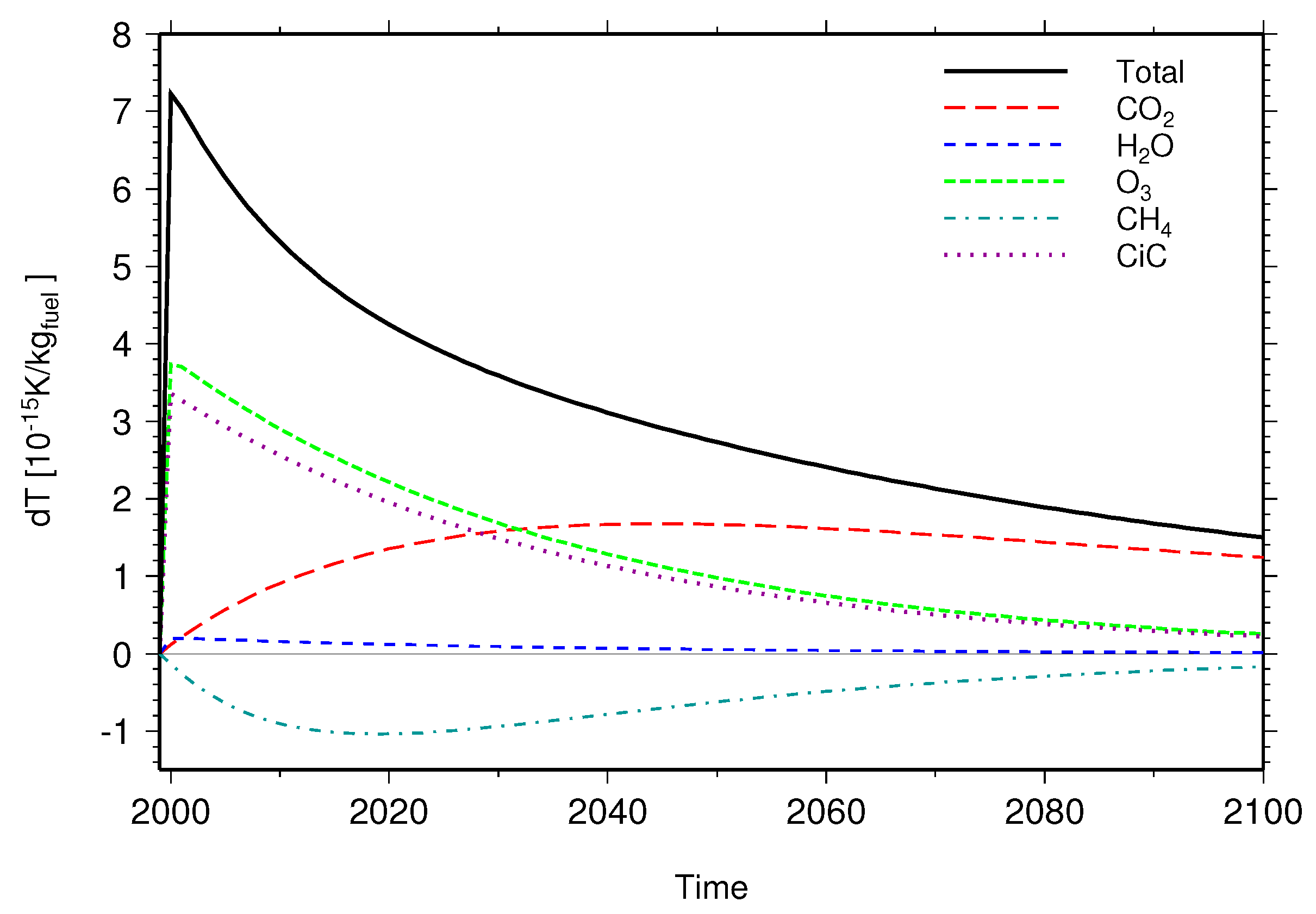
The provoked atmospheric perturbations alter the global average temperature on different time scales. Figure 1 exemplary shows the temporal evolution of global average temperature change $dT\left(t\right)$ for the forcing agents resulting from a one-year pulse emission in 2000 based on the REACT4C (Reducing Emissions from Aviation by Changing Trajectories for the benefit of Climate) emission inventory [31]. While the perturbations with short lifetimes (e.g., contrails and O${}_3$) decay relatively fast, long-lived components (e.g., CO${}_2$ and CH${}_4$) show a considerable impact over decades, even centuries (CO${}_2$). While the RF of CiC was the highest in Table 1, the temperature change of ozone is larger than that of CiC due to the different climate sensitivities: we assume for O${}_3$ climate sensitivity of 1.0 K·W${}^{-1}·$m${}^2$ and for CiC 0.43 K·W${}^{-1}·$m${}^2$ according to Ponater et al. [32]. These values are based on a few studies only and, hence, require further research.

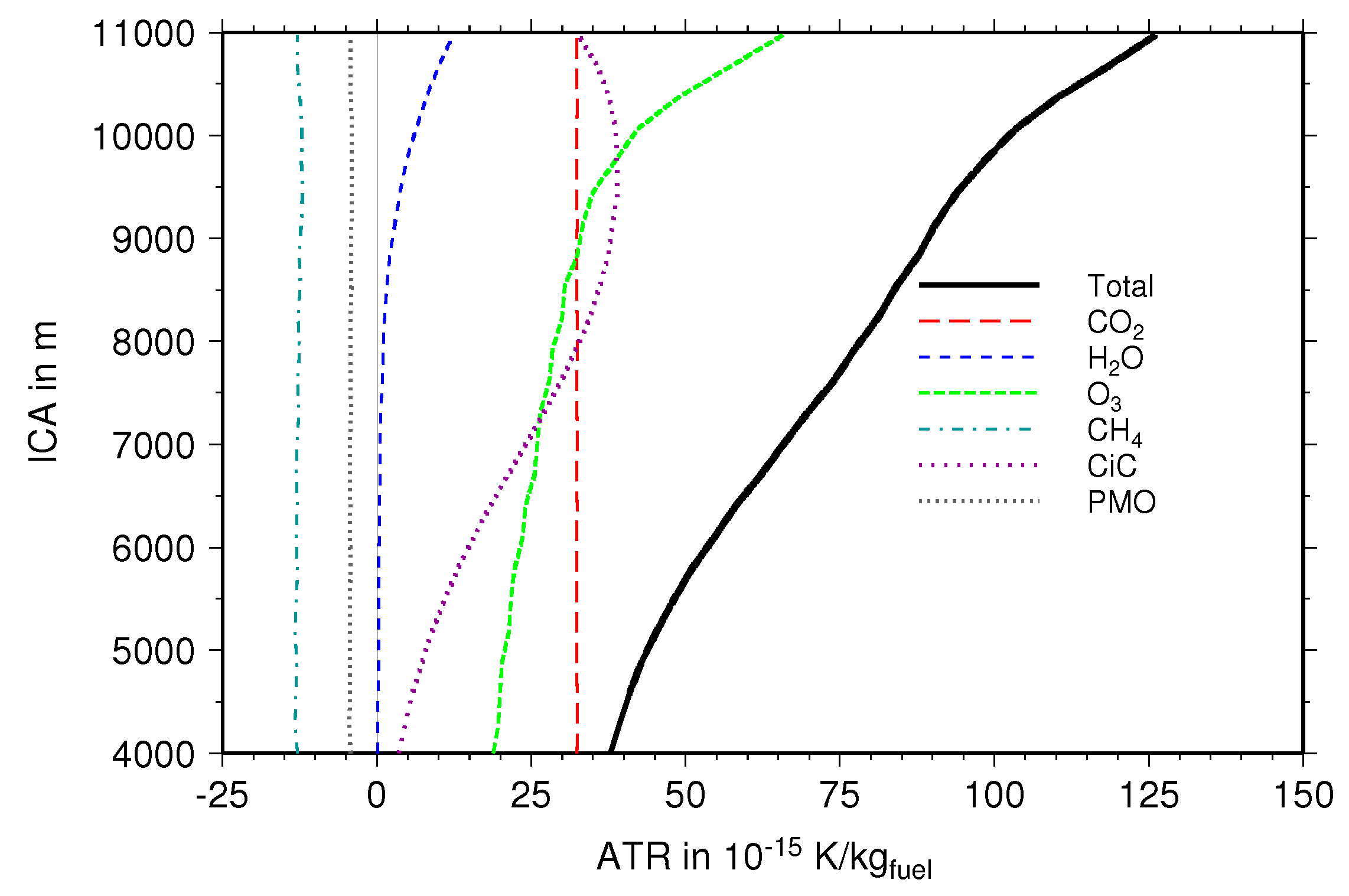
As the global average temperature response has a closer relation to weather events and climatic consequences than RF, it is more suited to measuring the future anthropogenic climate impact. The atmospheric response to the different emitted compounds further not only varies with time, but also depends on the locus of emission and underlying atmospheric conditions. Consequently, this compound-specific spatial dependency needs to be considered in the applied climate response model in order to correctly reflect the impact from aviation’s emissions. In this study, we use the climate response model AirClim [9,33,34,35,36], which analyzes the climate impact of CO${}_2$, H${}_2$O, CH${}_4$, O${}_3$ (short and long-lived) and CiC. AirClim considers the altitude and latitude dependency of the non-CO${}_2$ emissions, but is nevertheless computationally efficient to analyze the climate impact over a long time period (e.g., 100 years).

3. Model Description

The discussion about the climate impact of aviation shows that the systematic assessment of changes to current aircraft design and operations requires an adequate level of model fidelity and expertise to capture the relevant interdependencies among aircraft and engine performance, emissions, climate change and economics. Such a comprehensive simulation and analysis approach was developed in the DLR project CATS [14,37,38,39]. The integration framework, data model and disciplinary analysis models are provided by several DLR institutions and academia. The plausibility of the overall simulation results is ensured by the involved experts in a collaborative way. The superscript behind each model name shows the institute that provides the model and expertise. The list of all involved institutes is provided at the end of this article. These experts are usually not situated at the same location, but are regionally distributed. This leads to the need for a distributed design and analysis environment that links the required disciplinary analysis models and provides a means for remote triggering, overall process control, convergence monitoring and optimization. The CATS simulation workflow is based on the integration framework Remote Component Environment${}^{vii}$ (RCE) in combination with the Chameleon Suite${}^{vii}$ to link the different models [40]. The central data model Common Parametric Aircraft Configuration Schema (CPACS)${}^{ii}$ is used for flexible and efficient data exchange [41,42,43]. Both components are developed by DLR and available open source also to external research and industry institutions [44]. 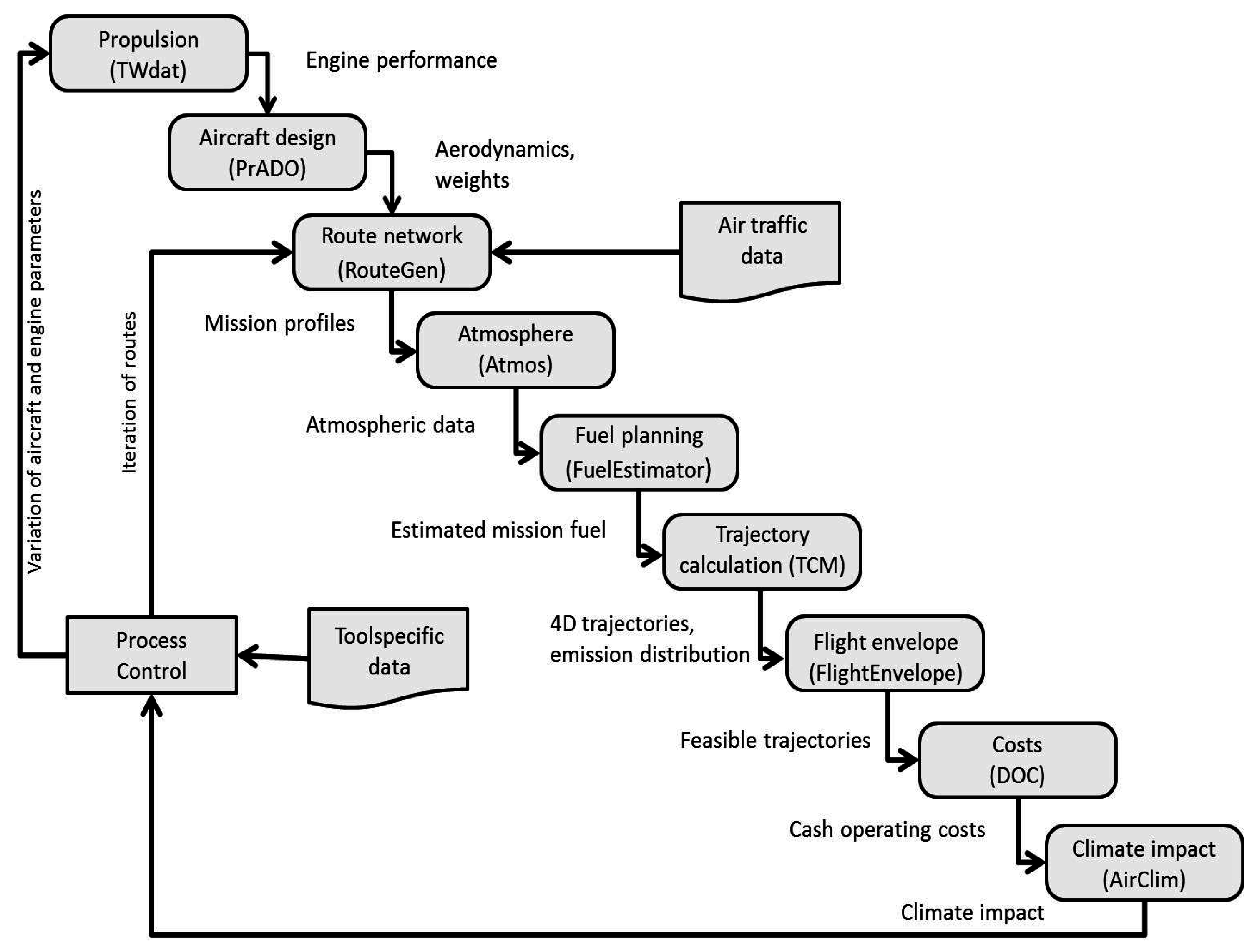Figure 2 shows the CATS simulation workflow with integrated analysis models and iteration paths for varying routes and/or aircraft design changes. Depending on the scope of studies, different process control scripts are activated for parameter variation or optimization studies. The calculation procedures in the CATS simulation workflow are as follows: the surrogate database model TWdat${}^{iii}$ provides engine performance tables for several generic engines representing today’s technology, as well as possible future propulsion concepts, which are pre-calculated by the well-established thermodynamic cycle program Varcycle${}^{iii}$ [45] and fitted to real engine data. These performance tables contain thrust and fuel flow characteristics, as well as emission indices from NO${}_{\mathrm{x}}$, soot and CO [46].

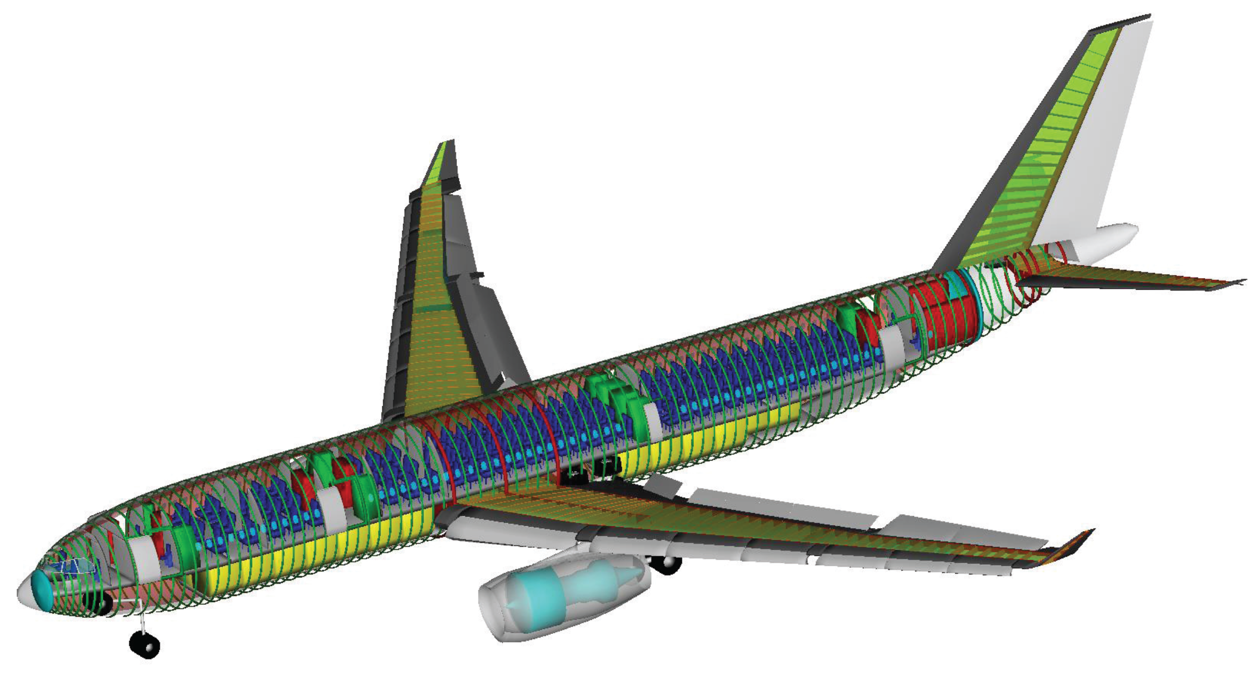
The multi-disciplinary aircraft design tool PrADO${}^{viii}$ (Preliminary Aircraft Design and Optimization) is applied to calculate the flight performance and technical characteristics of actual and novel aircraft configurations. PrADO comprises physical models with empirical extensions for aerodynamics, structural sizing, weight prediction and flight performance, including trim calculations and geometry description [47]. The tool also captures the influence of aircraft subsystems on engine performance through bleed air and shaft power extraction. The physics-based sub-models in PrADO, especially for structural sizing and aerodynamics, allow also the evaluation of aircraft configurations that are not covered by statistical relations, such as, e.g., a high aspect ratio wing configuration. Without any calibration on the given reference (real) data, PrADO typically provides estimates for the overall aircraft characteristics (aircraft weights, aerodynamic performance, etc.) in the range of 5%–10% for classical tube and wing configurations, which is, in the context of preliminary aircraft design, a good error margin.

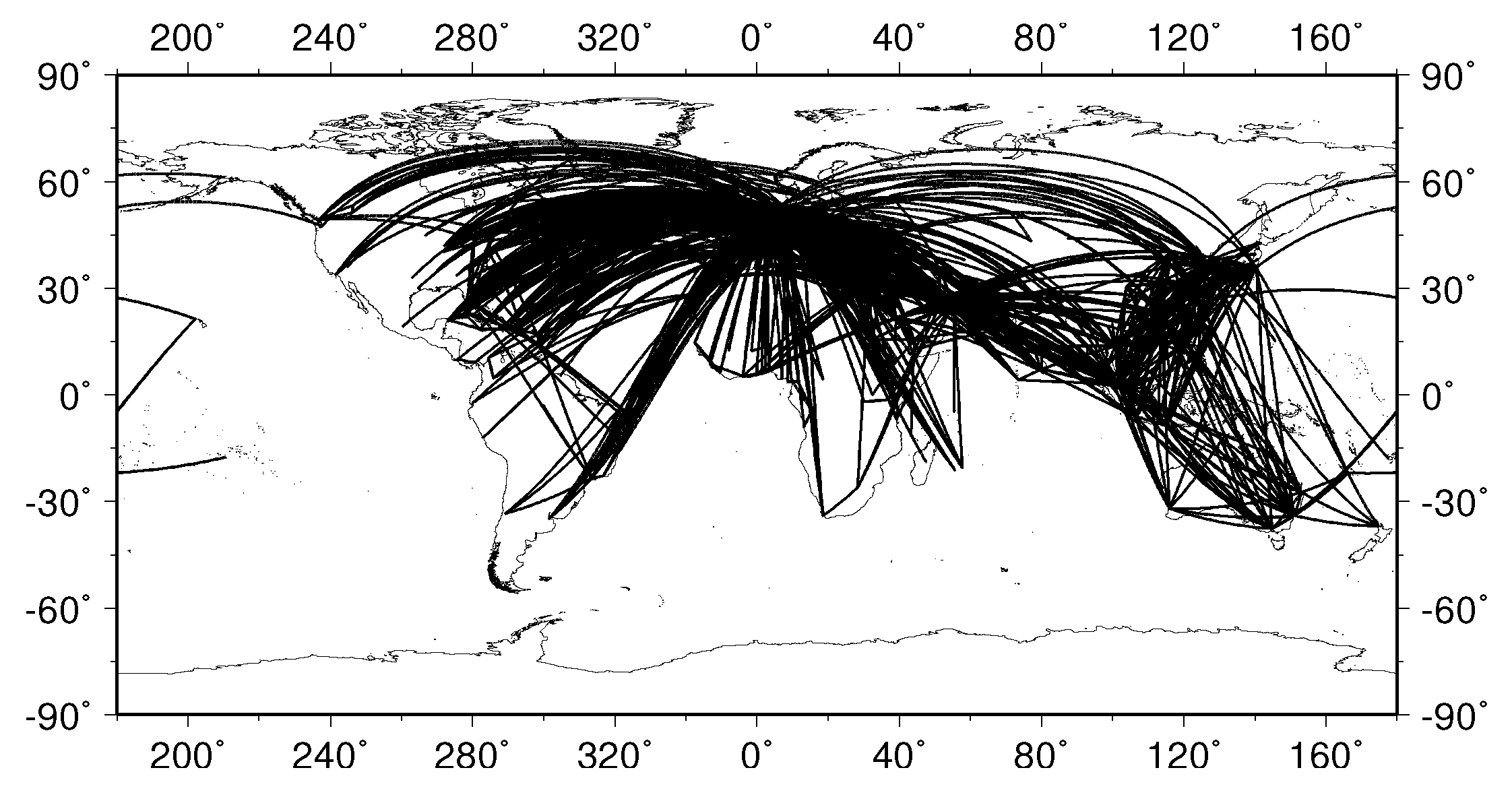
The preliminary flight preparation models RouteGen${}^{ii}$ and FuelEstimator${}^{ii}$ provide relevant data concerning the route description and mission profile (location of airport pairs, vertical and lateral flight path and annual flight frequencies), estimated mission fuel and resulting payload limitations for all analyzed routes [14].

Annual average atmospheric data along each route, including temperature, pressure and relative humidity (for EI${}_{\mathrm{N}{\mathrm{O}}_{\mathrm{x}}}$ (emission index of NO${}_{\mathrm{x}}$) correction) as a function of latitude and altitude are provided by the model Atmos${}^i$. Therefore, we use the five-year mean of the DLR climate-chemistry model E39/CA (ECHAM4.L39(DLR)/CHEM-ATTILA) output.

The Trajectory Calculation Module (TCM)${}^{ii}$ is applied to calculate the four-dimensional (latitude, longitude, altitude, time) trajectory and corresponding emission distributions [49,50]. TCM performs a fast-time simulation that integrates the relevant flight conditions based on the BADA (Base of Aircraft Data) total energy model [51]. Input data comprise the mission parameters, such as vertical profile and horizontal flight path definitions, the aircraft weight breakdown, as well as engine and aerodynamic performance tables for different high-lift configurations provided by TWdat and PrADO. This also enables the flight performance and trajectory simulations of novel aircraft concepts. The flight path is defined by given lateral waypoints, whereas the vertical profile consists of several segments, each characterized by specific target aircraft state conditions that are derived from standard flight procedures.

The FlightEnvelope${}^{ii}$ checks for each calculated trajectory whether the aircraft specific flight performance envelope is violated with regard to stall, buffet limits or cruise altitude capability. In case of such a violation, the concerning trajectory is disregarded in the simulation [14].

For each trajectory without such a violation, the COC (cash operating costs) per flight are evaluated by the DOC${}^{ii}$ (Direct operating cost) model, which includes the costs for fuel, crew, maintenance, navigation and landing fees [52].

The climate impact of each flight is assessed with the climate response model AirClim${}^i$ [9,33,34,35,36]. AirClim is designed to be applicable to aviation studies, considering the impact of the altitude and latitude of emission on the climate impact of CO${}_2$, H${}_2$O, CH${}_4$, O${}_3$ (short- and long-lived) and CiC. The model comprises latitude- and altitude-dependent response functions of a climate-chemistry model from the emission to RF, resulting in an estimate in near surface temperature change. Combining aircraft emission data with a set of previously-calculated atmospheric perturbations, AirClim calculates the RF and resulting temporal evolution of global near surface temperature change over a specified time horizon. The pre-calculated data are derived from 85 steady-state simulations for the year 2000 with the DLR climate-chemistry model E39/CA, prescribing normalized emissions of NO${}_{\mathrm{x}}$ and H${}_2$O at various atmospheric regions [9]. An overview of the latitude and altitude dependency of the climate impact of different emissions can be found in the appendix of Dahlmann et al. [36]. As there are still many uncertainties in the calculation of the climate impact of air traffic [1], AirClim includes a Monte Carlo simulation and analyzes relative differences between scenarios (described in Section 4) in order to derive a reliable assessment of climate impact mitigation potentials [36].

The developed model workflow is extendable to other climate impact assessments of air traffic through the integration of additional analysis models via the central data model CPACS and the flexible design framework RCE/Chameleon.

4. Evaluation Methodology

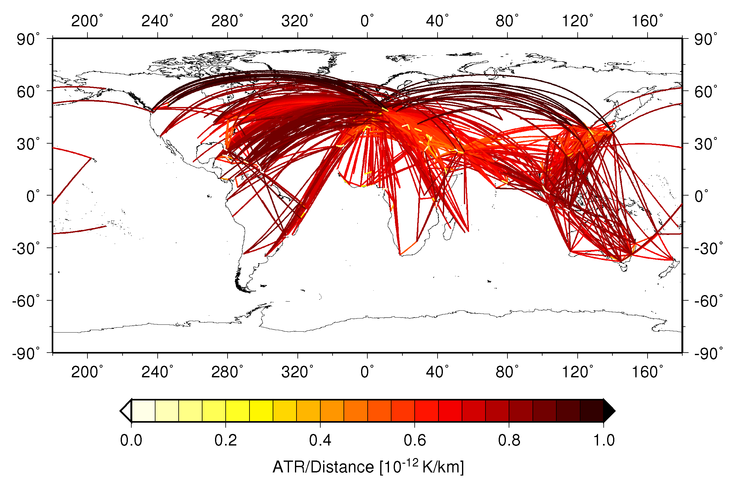
As outlined above, changes of the current cost-optimized state of air transport towards reduced climate impact often cause cost penalties due to increased fuel burn or travel time. An evaluation of possible climate impact mitigation strategies should be conducted as a cost-benefit analysis that allows for the identification of the most cost-efficient measure. In this sense, the present study applies the COC for the economic assessment and the ATR (average temperature response) [13] as the climate impact metric for each simulated flight. ATR is the average global surface temperature change dT(t) over a defined time horizon H according to Equation (1):

$${\mathrm{ATR}}_H=\frac{1}{H}\underset{t}{\overset{t+H}{\int }}dT\left(t\right)dt$$

(1)

The CATS assessment is split into three sequential analysis steps. First, the climate impact mitigation potential resulting from flight altitude and speed changes with the defined reference aircraft is analyzed on each route individually. Therefore, numerous cruise operating conditions are simulated for each route in the global route network with the outlined simulation workflow and settings. For each route (index i), variations of $M{a}_{cr}$ and initial cruise altitude (ICA) are conducted (see

Table 2. Range of parameter variations (initial cruise altitude (ICA), Mach number at cruise flight ($M{a}_{cr}$)) applied in the present study to derive the operational mitigation potential.

Parameter	Minimum Value	Maximum Value	Step Width
ICA (m)	3965	12,200	305
$M{a}_{cr}$	0.4	0.85	0.01

). For each trajectory (feasible ICA, $M{a}_{cr}$ combination (Mach number at cruise flight), index k), the changes of ATR${}_{i,k}$ and COC${}_{i,k}$ are expressed relative to the route-specific reference trajectory (see Section 5.3).

$${\mathrm{COC}}_{rel,i,k}=\frac{{\mathrm{COC}}_{i,k}}{{\mathrm{COC}}_{i,ref}}$$

(2)

$${\mathrm{ATR}}_{rel,i,k}=\frac{{\mathrm{ATR}}_{i,k}}{{\mathrm{ATR}}_{i,ref}}$$

(3)

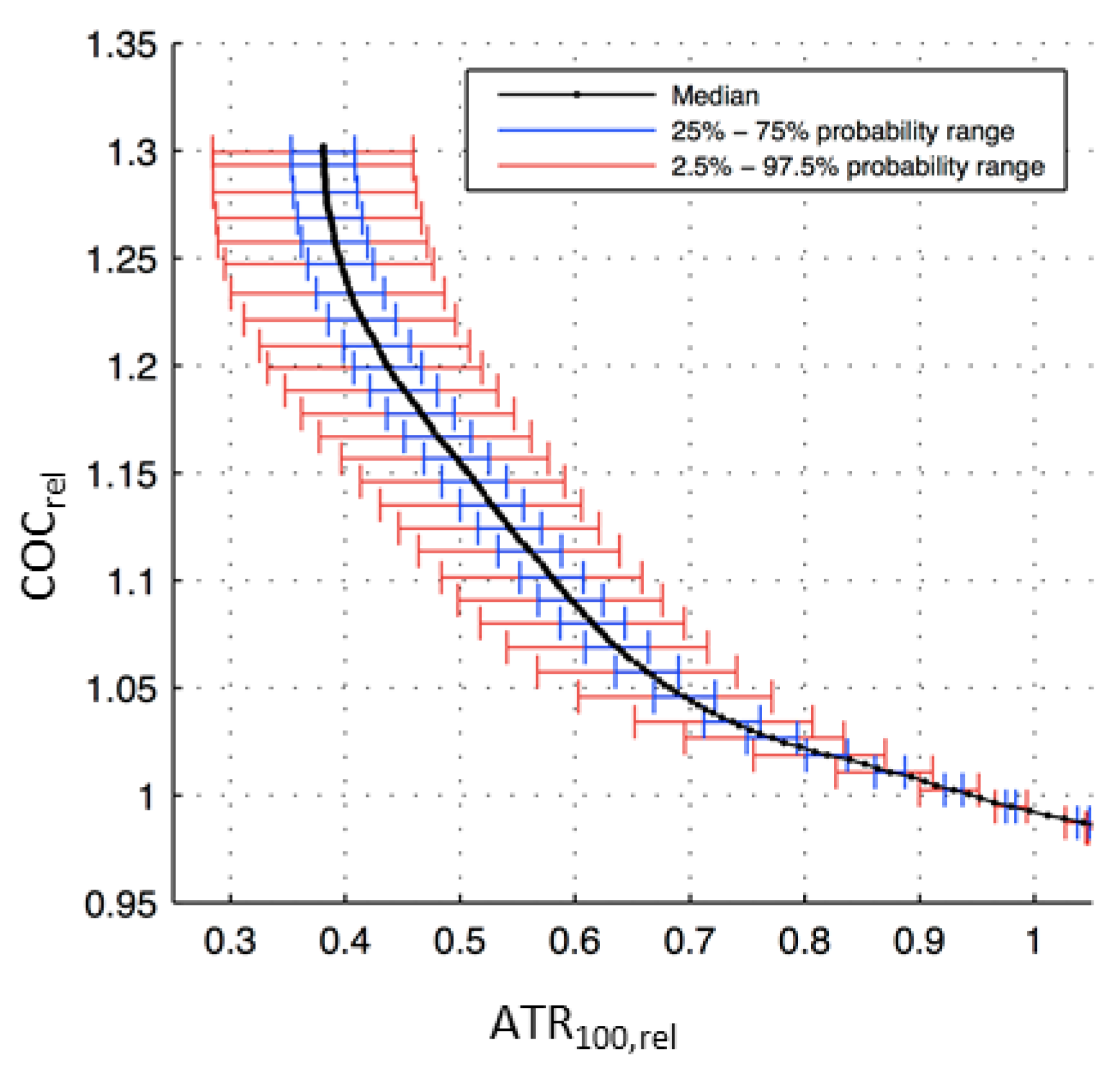
Expressing further the relative changes for all analyzed trajectories (k on route i) as cost-benefit ratio ATR${}_{rel,i,k}$ vs. COC${}_{rel,i,k}$ provides a Pareto front (P) with ICA and $M{a}_{cr}$ combinations that maximize the mitigation potential for given cost penalties on route i, which is defined as:

$$F:X\subset R^2\to Y\subset R^2$$

(4)

$$f:X=(M{a}_{cr},\mathrm{ICA})\to Y=(\mathrm{ATR},\mathrm{COC})$$

(5)

$$P=\{y=(y_1,y_2)\in Y\mid x\in X:\exists f\left(x\right)=y\wedge \forall x\in X:(f_1\left(x\right)<y_1\vee f_2\left(x\right)<y_2)\}$$

(6)

For the following evaluation steps, only the ICA and $M{a}_{cr}$ combinations on the Pareto fronts are taken into account. The mitigation potential is only given at discrete values of relative cost changes, as interpolation between the given Pareto elements is not possible without the loss of information concerning the calculated confidence interval of ATR. The relative changes of climate impact and COC differ for each route, hence altering the mitigation potential obtained at the given cruise condition. To obtain the mitigation potential for the global route network with n routes (index $all$) at a given global relative cost change COC${}_{rel,i}=x$, every route-specific Pareto front is intersected at the specified value of x and evaluated at the next smaller available Pareto element ${x_i}^{\prime }$. The route-specific relative climate impact reductions ATR${}_i$(${x_i}^{\prime }$) are summed for all n routes after being weighted by the route-specific flight frequency $f_i$ (see Equation (7)). The same approach is applied to determine the resulting global change of COC${}_{rel,all}\left(x\right)$ (see Equation (8)).

$${\mathrm{ATR}}_{rel,all}\left(x\right)=\frac{{\displaystyle \sum _{i=1}^n}{f}_i·{\mathrm{ATR}}_i\left(x_i^{\prime }\right)}{{\displaystyle \sum _{i=1}^n}{f}_i·{\mathrm{ATR}}_{i,ref}}$$

(7)

$${\mathrm{COC}}_{rel,all}\left(x\right)=\frac{{\displaystyle \sum _{i=1}^n}{f}_i·{\mathrm{COC}}_i\left(x_i^{\prime }\right)}{{\displaystyle \sum _{i=1}^n}{f}_i·{\mathrm{COC}}_{i,ref}}$$

(8)

The application of this calculation for all cost changes (x) between the minimum and maximum values of COC${}_{rel,i}$ provides the Pareto front for the global route network and world fleet of the analyzed aircraft (see Section 6).

In the second step, the frequency distribution of cruise flight conditions (i.e., ICA and $M{a}_{cr}$) that corresponds to an accepted global cost change COC${}_{rel,all}$ is assessed to derive new design conditions for future aircraft with reduced climate impact. Therefore, each route-specific Pareto front is intersected at the defined cost change (x) and evaluated for the next smaller available Pareto element on the curve, providing the climate impact reduction ATR${}_{rel,i}$(${x_i}^{\prime }$), as well as the corresponding cruise condition ICA${}_i$(${x_i}^{\prime }$) and $M{a}_{cr,i}$(${x_i}^{\prime }$). Applying this procedure to all routes of the global route network provides the normalized frequency distribution ${\mathsf{\Phi }}_x$(ICA, $M{a}_{cr}$) of cruise conditions (see Equation (9)), where ${\delta }_i$(ICA, $M{a}_{cr}$) indicates the occurrence of a given operating point on the Pareto front of route i at cost penalty x (see Equation (10)). Each occurring cruise condition is weighted with the route-specific absolute climate impact mitigation potential ($=f_i·\left(1-{\mathrm{ATR}}_{rel,i}({x_i}^{\prime })\right)·{\mathrm{ATR}}_{i,ref}$).

$${\mathsf{\Phi }}_x(\mathrm{ICA},M{a}_{cr})=\frac{{\displaystyle \sum _{i=1}^n}{f}_i·(1-{\mathrm{ATR}}_{rel,i}\left(x_i^{\prime }\right))·{\mathrm{ATR}}_{i,ref}·{\delta }_i(\mathrm{ICA},M{a}_{cr})}{{\displaystyle \sum _{i=1}^n}{f}_i·(1-{\mathrm{ATR}}_{rel,i}\left(x_i^{\prime }\right))·{\mathrm{ATR}}_{i,ref}}$$

(9)

$${\delta }_i(\mathrm{ICA},M{a}_{cr})=\left\{\begin{array}{cc}1,\hfill & \mathrm{ICA}={\mathrm{ICA}}_i\&Ma=M{a}_{cr,i}\hfill \\ 0,\hfill & else\hfill \end{array}\right.$$

(10)

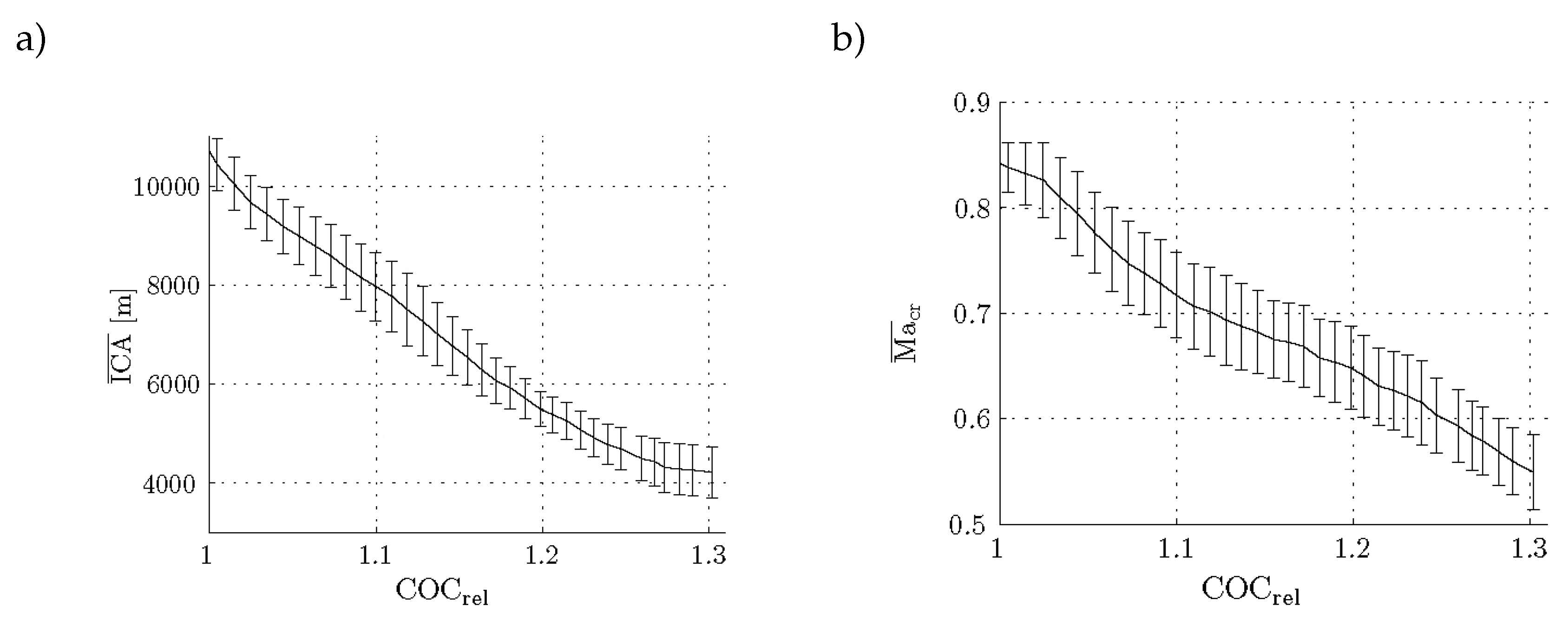
The average $\overline{M{a}_{cr}}$ and $\overline{\mathrm{ICA}}$ result from the frequency distribution ${\mathsf{\Phi }}_x$(ICA, $M{a}_{cr}$) corresponding to a specified cost change x.

$$\overline{\mathrm{ICA}\left(x\right)}=\sum _{\mathrm{ICA},M{a}_{cr}}{\mathsf{\Phi }}_x(\mathrm{ICA},M{a}_{cr})·\mathrm{ICA}$$

(11)

$$\overline{M{a}_{cr}\left(x\right)}=\sum _{\mathrm{ICA},M{a}_{cr}}{\mathsf{\Phi }}_x(\mathrm{ICA},M{a}_{cr})·M{a}_{cr}$$

(12)

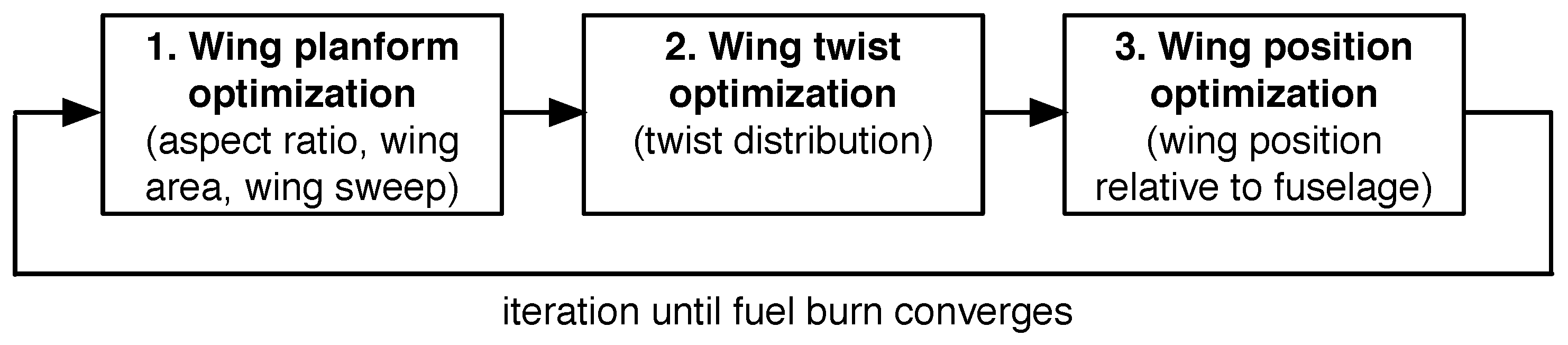
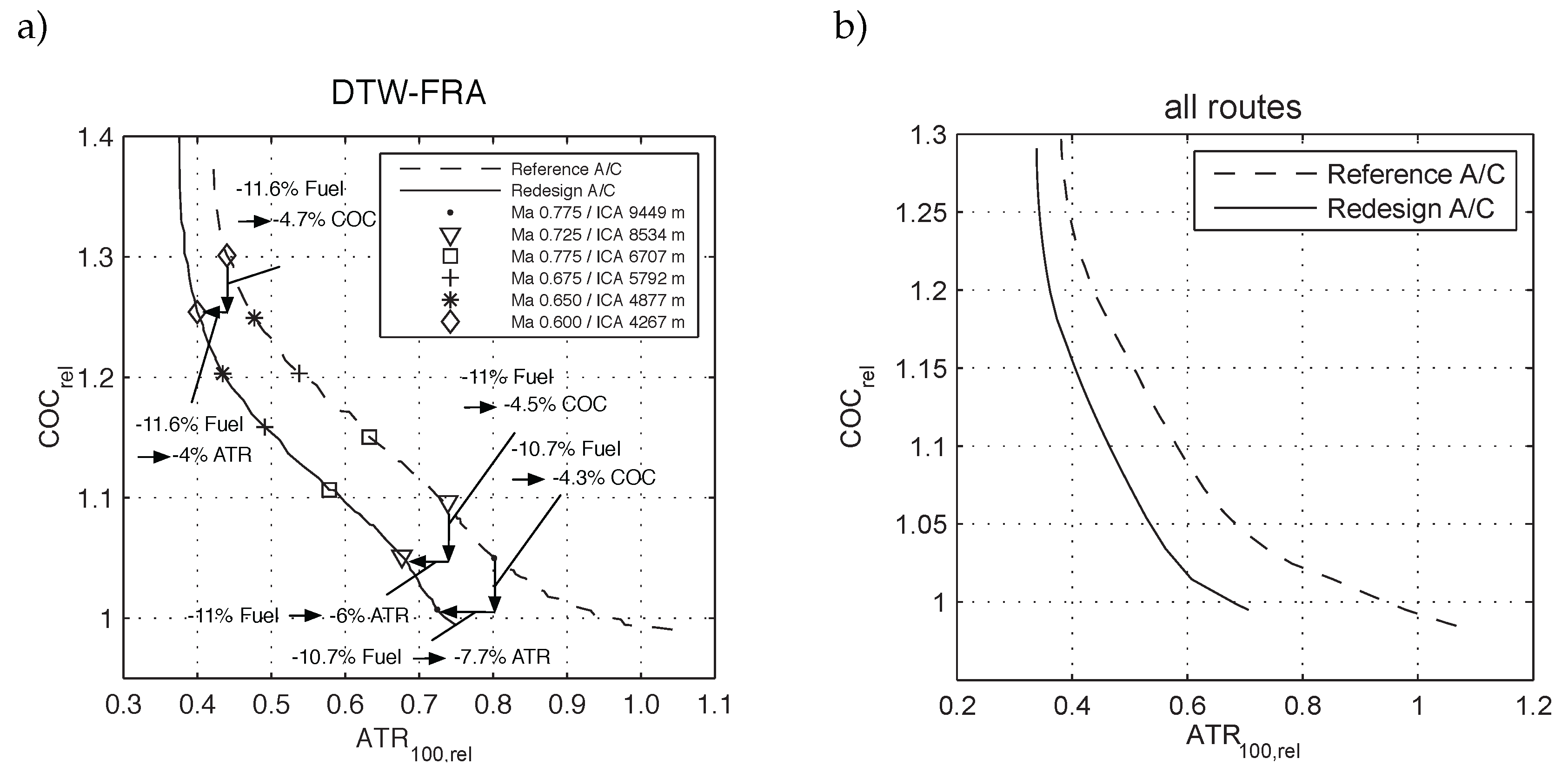
In a third step, the reference aircraft is optimized with respect to fuel burn for the new design conditions and re-assessed with the outlined model workflow in order to derive the additional potential given by aircraft design changes. Combining operational and aircraft design changes provides an estimate for the climate impact mitigation potential and related costs for a future climate-compatible air transport system. In aircraft design studies, the top level aircraft requirements (TLAR) describe the target performance parameters for a new aircraft, including the payload-range capabilities, high and low speed performances, etc. The TLAR further contains the definition of ICA and $M{a}_{cr}$ as target condition for the optimization of the aircraft high-speed performance. Both parameters serve as new design conditions for aircraft configurations, which are optimized with respect to fuel burn for adapted cruise conditions with reduced climate impact. In order to identify the mitigation potential solely rooted in aircraft design changes, the optimization is conducted with a constant technology level, an engine performance map and payload-range capabilities. Based on these requirements, the optimization procedure focuses on the modification of the wing geometry and is organized as an iterative three-step approach. In each step, PrADO calculations (see Section 3) for a set of varying geometry parameters are performed (see Figure 3). Based on this, kriging surrogate models are constructed [53]. The optimal geometry parameter set is then obtained by applying brute-force techniques to the surrogate model.

5. Reference Scenario

Dahlmann et al. [36] and Grewe and Dahlmann [54] demonstrated that the climate impact mitigation potential is best analyzed with respect to a given reference air traffic scenario in order to reduce the uncertainties related to the assessment of component-specific temperature responses. This section describes the reference conditions and assumptions applied for the analyses.

5.1. Aircraft-Engine Configuration

The Airbus A330-200 equipped with CF6-80E1A3 engines is selected as the reference aircraft, as it is the most sold aircraft in the medium- and long-range category, besides the Boeing 777. The external geometry, cabin configuration and structural layout are modeled by PrADO according to the real aircraft. The predicted aircraft component weights and drag polar are fitted to available manufacturer data by corresponding scaling factors. TWdat provides the performance data for the selected engine type. Figure 4 shows the geometry model of the reference aircraft.

Table 3. Top level design requirements for the reference aircraft A330-200 and its model characteristics. PAX: passenger; FAR: federal aviation regulation; L/D: lift-to-drag ratio; TSFC: the specific fuel consumption.

Design Criteria		Model Characteristics
Range with max payload	7860 km	Operational empty weight	115,700 kg
Ferry range	17,000 km	Max take-off weight	221,600 kg
Passengers (3 classes)	253 PAX	FAR take-off field length	2391 m
Max payload	49,000 kg	FAR landing field length	1688 m
ICA	10,000 m	Approach speed	75.5 m/s
Max. cruise altitude	12,500 m	L/D@design conditions	19.9
Design cruise Mach No.	0.82	TSFC@design conditions	0.05728 g/N/h

summarizes the basic model design criteria and performance characteristics of the aircraft. More details can be found from Koch [14]. The following trajectory calculation considers an average passenger load factor of 0.76 and 5000 kg of additional cargo [55], which corresponds to a typical operational payload.

5.2. Global Route Network

The global route network contains all passenger flights operated by the reference aircraft type (A330-200) in 2006, which results in a set of 1178 globally-distributed airport pair connections with corresponding flight frequencies derived from OAG (Official Airline Guide) data [56]. Figure 5 shows the analyzed global route network. As the present study is conducted without any wind influence during trajectory calculations, flight frequencies for outbound and inbound flights between the same origin-destination pairs are bundled. Despite neglecting wind fields, the climate impact of inbound and outbound flights differs, as emission amounts at the beginning are higher than at the end, and emission altitude increases with time.

5.3. Vertical Flight Profile

The modeled vertical flight profile includes several flight phases based on typical air traffic management (ATM) procedures and considers the common speed and altitude constraints during climbing and descending. The cruise phase is modeled as continuous climb cruise with a constant lift coefficient. Although this is a simplification of current flight procedures, it is considered as a valid approximation to a real cruise flight with step climbs, which are normally optimized by flight planning tools considering actual loading conditions and air traffic management restrictions. Such an optimization was infeasible in the scope of the present study.

Each simulated flight trajectory is checked for aircraft-specific flight envelope violations, including speed and altitude limitations, buffeting and stall limits. To derive the reference initial-cruise conditions for each route, real flight plans submitted to Eurocontrol’s Central Flow Management Unit (CFMU) are analyzed. The available data cover three full days of flight movements of the reference aircraft within the initial flight plan zone, which comprises all flights to, from or through European airspace. This results in 1476 flights, which are clustered by mission distance (the great circle between origin and destination) into groups of a 250-km step width. For each flight, the ICA and speed requested by the airline is identified. The reference cruise conditions are thus obtained as median value from the frequency distribution of each cluster [14,48].

5.4. Cost Assessment

The total operating costs (TOC) contain direct operating costs and indirect operating costs (IOC). IOC contains costs for ground installation, merchandise, etc., and roughly represents one third of the TOC [57]. The DOC includes COC (which are used in this study), as well as the costs for ownership. The costs of ownership (depreciation, interests and insurance) are about 20% of the DOC [57] and are not considered in this study, as the impact of flight speed changes on the aircraft utilization is highly dependent on the concrete airline-specific flight plans and airport restrictions. Such an impact evaluation requires detailed flight planning and airline fleet rotation models that were not available for this study.

The COC are calculated for each flight (USD/cycle); the COC represents the cost for fuel, maintenance, crew and fees (landing and navigation). The cost values for labor (25 USD/h) and fees are based on Liebeck et al. [52] and scaled by the average U.S. inflation rate (2.66%) between 1993 and 2006 [58]. The reference average fuel price in 2006 is set to 0.595 USD/kg [59]. The largest regional differences in fuel price (relative to the reference value in 2006) are derived from IATA (International Air Transport Association) fuel price data [60] and found to be within the bounds of −3.7% and +6.4%.

5.5. Climate Impact Assessment

The climate impact evaluation considers sustained emissions over 32 years (2006–2038), which corresponds to the average lifetime of the reference aircraft [55]. The evolution of background emissions of CO${}_2$ and CH${}_4$ follows the IPCC (Intergovernmental Panel of Climate Change) Scenario A1B, which is based on the assumption of an economically-oriented world with balanced use of fossil and renewable energies [61]. The background air traffic scenario for contrail cirrus assessment is based on data from the QUANTIFY emission inventory [62]. The development of the emissions refers to IPCC Scenario Fa1, which is a reference scenario developed by the ICAO (International Civil Aviation Organization) Forecasting and Economic Support Group (FESG) with mid-range economic growth from IPCC (1992) and technology for both improved fuel efficiency and NO${}_{\mathrm{x}}$ reduction [15]. The ATR is calculated for the time frame of H = 100 years (ATR${}_{100}$) starting in 2006.

6. Results

6.1. Status Quo: Results for the Reference Scenario

Analyzing the reference scenario with the outlined model workflow and settings provides the ATR per route and flown km, as shown in Figure 6. The short-haul routes with flight distances below 1000 km show a lower ATR per km, which comes from lower cruise altitudes and resulting lower impacts of O${}_3$, H${}_2$O and CiC. Flights with distances above 1000 km show ICAs between 10,000 m and 12,000 m.

The ICA decreases for longer flight distances due to the increased aircraft take-off weight. However, the average cruise altitudes for long-range flights are very similar for all flight distances as the altitude difference between the start and end of cruise increases with an increase of flight distance, compensating thus the lower ICA. In combination with the fact that the average tropopause altitude decreases towards higher latitudes, flights at a given altitude cause a larger climate impact at higher latitudes due to the increased impacts from H${}_2$O and reduced depletion rates of CH${}_4$. The opposite is observed for the flights conducted at lower latitudes, where the tropopause is on average above typical cruise altitudes. An exception to this pattern is observed for the flights between Europe and North America, which exhibit a lower climate impact than the flights between Europe and Central America. The large amount of flights in the north Atlantic region leads to saturation effects of CiC and impacts the route-specific climate impact in the applied climate response model [34]. The same effect is observable on highly-frequented routes in southwest Asia.

6.2. Climate Mitigation Potential Given by Altered Cruise Conditions with Current Aircraft

The largest potential to reduce climate impact is for long-range flights, which provide the highest flexibility for operational changes. Among the different flight phases, the cruise phase contributes most to the climate impact of each flight due to its altitude and its share of mission fuel and emitted pollutants. Additionally, the cruise phase presumably offers the highest flexibility for altitude (and speed) changes, compared to other flight phases that are more restricted by ATM constraints. To quantify the climate impact mitigation potential for current aircraft, numerous flight trajectories under different cruise operating conditions are simulated for each route in the global route network. Table 2 shows the range parameter for ICA and $M{a}_{cr}$. ATR and COC were analyzed for each combination of $M{a}_{cr}$ and ICAs (trajectory). Note that the wide ranges of ICA and $M{a}_{cr}$ values are chosen to investigate the maximum potential of climate impact reduction over the full range of feasible cruise flight conditions.

Figure 7 shows the resulting Pareto front (black line) for the route Detroit-Frankfurt (DTW-FRA) as an example. The Pareto front shows a considerable potential to reduce the climate impact of air traffic with small to moderate increased COC. Figure 8 depicts the resulting Pareto front ATR${}_{rel,all}$ vs. COC${}_{rel,all}$ for all analyzed routes operated by the reference aircraft. Most route-specific reference cruise conditions are not part of the Pareto front. Hence, it is possible to reduce the climate impact without a COC increase until the analyzed ICA and $M{a}_{cr}$ combination becomes part of the Pareto front. Summed for all routes, this effect provides a COC neutral ATR reduction of 5% relative to the reference conditions. However, the magnitude of this effect depends on the applied model assumptions and sensitivities, like the increase of fuel burn with Mach number with altitude vs. climate impact reduction with altitude.

The climate impact in terms of ATR of the different climate agents per kg consumed fuel with the dependency of ICA is exemplarily shown in Figure 9 for the route DTW-FRA. It shows that the combined climate impacts reach a minimum at the lowest flight levels and are largest for flights in the stratosphere, mainly because of large contributions from O${}_3$ and H${}_2$O. The climate impact of CiC is highest in the upper troposphere and smaller in the dry stratosphere and in the warmer lower troposphere, but the differences are not large enough to cause a secondary minimum in the stratosphere, in the applied climate response model. A discussion of the reliability of the resulting altitude dependency of the climate impact can be found in Section 8.

Table 4. Mitigation potentials and efficiencies relative to the reference cruise conditions. Related average $\overline{\mathrm{ICA}}$ and $\overline{M{a}_{cr}}$ combinations are derived from the frequency distribution resulting at a given COC increase.

COC Increase (%)	ATR Reduction (%)	Mitigation Efficiency	$\overline{\mathbf{ICA}}$ (m)	$\overline{{\mathit{Ma}}_{\mathit{cr}}}$
neutral	5	-	11,278	0.814
1	11	11.0	10,188	0.836
5	31	6.2	9065	0.783
10	42	4.2	7974	0.717
20	56	2.8	5460	0.649
30	62	2.1	4221	0.549

summarizes the resulting ATR${}_{rel,all}$ values for selected cost penalties (COC${}_{rel,all}$) with corresponding $\overline{\mathrm{ICA}}$ and $\overline{M{a}_{cr}}$ values derived from the respective frequency distributions. Table 4 further highlights that the mitigation efficiency, which expresses the ratio of achievable ATR reduction per COC increase, is especially favorable for small COC changes. For a 10% COC change, the climate impact can be reduced by 42%. While the climate impact decreases with decreasing altitude (Figure 9), the COC increases because of increased fuel consumption and longer flight times. Calculating the average $\overline{\mathrm{ICA}}$ and $\overline{M{a}_{cr}}$ values for each COC increment provides Figure 10, which depicts decreasing cruise altitudes and Mach numbers for increasing cost penalties.

As discussed above, current aircraft are optimized for today’s typical cruise conditions. The operation at lower altitudes and speeds, hence under the off design conditions, causes performance losses that result in increased fuel burn and mission times. Figure 11 depicts the evolution of average mission fuel and mission time values (flight frequency weighted fleet average) as a function of increasing COC (and related ATR) changes.

The figure highlights that the climate impact can be reduced, although fuel burn and the related CO${}_2$ impact are increasing. This results primarily from the reduced impact of NO${}_{\mathrm{x}}$ and CiC at lower altitudes in the present model [34]. On the other side, the increase of mission time and fuel raises the COC per flight. As fuel cost plays a considerable role in airline economics, it is therefore essential to minimize the fuel-burn penalty experienced by current aircraft operated at lower cruise altitudes and Mach numbers through redesigning the aircraft for these new cruise conditions. Reducing the fuel penalty will lead to an additional climate impact reduction due to decreased CO${}_2$ and NO${}_{\mathrm{x}}$ emissions.

6.3. Climate Mitigation Potential Given by Aircraft Design Optimization

The present study exemplarily considers the 10% COC penalty case for aircraft optimization studies. Analyzing the corresponding cumulated frequency distribution of cruise altitudes and speeds reveals that the reference aircraft is operated on average at $\overline{\mathrm{ICA}}$ = 7974 m and $\overline{M{a}_{cr}}$ = 0.717 [14]. The reference configuration is thus optimized with respect to fuel burn for ICA${}_{Design}$ = 8000 m and $M{a}_{cr,Design}$ = 0.72 with PrADO and TWdat. The maximum operating altitude is set to 10,500 m and the maximum operating speed to $Ma$ = 0.78. The optimization procedure focuses on the modification of the wing geometry while maintaining important performance characteristics of the reference aircraft (i.e., payload, range, control and stability margins, airport restrictions). Based on this requirements, the fuselage and cabin layout are kept identical to the reference aircraft. Instead, the wing sweep, aspect ratio, wing area and spanwise twist distribution are optimized for the new operating conditions. Further, the leading edge (LE) sweep angle and area of the vertical and horizontal tail planes are adapted according to the wing planform changes assuming a constant tail volume coefficient and identical relative sweep changes. Figure 12 depicts the geometrical changes of the redesigned configuration in comparison to the reference aircraft.

Table 5. Key design parameters for the reference and redesigned aircraft under initial cruise conditions. LE: leading edge; HTP: horizontal tail plane; VTP: vertical tail plane; OWE: operational empty weight; MTOW: maximum take-off weight; TOFL: take-off field length; LFL: landing field length.

Geometry	Reference	Redesign
Wing area (m${}^2$)	362	360
Wing span (m)	60	71
Wing LE sweep angle ($°$)	32	22
Wing aspect ratio (excluding Winglets)	9	13
HTP area (m${}^2$)	72	59
HTP LE sweep angle ($°$)	34	24
VTP area (m${}^2$)	53	64
VTP LE sweep angle ($°$)	44	31
Performance	Reference	Redesign
OWE (t)	116	120
MTOW (t)	222	224
FAR TOFL (m)	2391	2249
FAR LFL (m)	1688	1796
Approach speed (m/s)	76	74
L/D@design conditions	20	23
Lift coeffcient@design conditions	0.466	0.463
TSFC@design conditions (kg/N/h)	5.728 × 10${}^{-2}$	5.827 × 10${}^{-2}$

shows key design parameters for the reference and redesigned aircraft operated at ICA = 8000 m with $Ma$ = 0.72 on the design mission [14].

The redesigned configuration shows a decreased leading edge sweep angle of the wing, horizontal and vertical tail plane according to the lower Mach number (Table 5). The wing span increases at nearly constant wing area, which leads to the increased aspect ratio and improved aerodynamic efficiency (lift-to-drag ratio (L/D)) by 15%, but also increased wing weight. According to the empirical relations applied during the optimization, the area of the horizontal tail plane (HTP) decreases due to the increased lever, whereas the vertical tail plane (VTP) area increases due to the increased wing span and engine lever. The fuselage weight decreases due to the lower pressure difference under the new design cruise conditions. In total, the operational empty weight (OWE) increases by 4%. Despite the increased OWE, the improved aerodynamic efficiency leads to reduced thrust required during cruise flight. The specific fuel consumption (TSFC) increases slightly by 1.7% as a result of engine performance losses at the new cruise conditions. In combination, both effects lead to a reduction in mission fuel of 11% (on its aircraft design mission trajectory) compared to the reference aircraft operated at the new design mission.

The climate impact mitigation potential for the redesigned aircraft operated at lower cruise altitudes and speeds is determined in analogy to the reference aircraft. The cruise conditions are varied for each route according to

Table 6. Range of ICA and $M{a}_{cr}$ variations applied in the present study to derive the operational mitigation potential of the redesigned aircraft.

Parameter	Minimum Value	Maximum Value	Step Width
ICA (m)	3965	10,500	305
$M{a}_{cr}$	0.4	0.78	0.01

.

Computing the COC and ATR changes for each trajectory relative to the route-specific reference trajectory shows a considerable improvement in costs and climate impact due to the increased fuel efficiency compared to the reference aircraft. Figure 13 depicts the Pareto fronts for the reference and redesigned aircraft resulting for the route DTW-FRA and the global route network.

The comparison of the selected cruise conditions for DTW-FRA shows that the fuel-burn improvement of 10%–11% leads to a 4%–5% reduction of COC, which is in good agreement with the average share of fuel costs on total COC (Figure 13a). The fuel-burn reduction further reduces ATR by 4%–8% (depending on ICA) due to the lower amounts of emitted pollutants. The trends observed for DTW-FRA are also visible in the Pareto front for the global route network (Figure 13b). It shows that for the selected 10% COC penalty, the ATR reduction increases from 42%–54%. Considering the importance of economic efficiency for the airlines, it is rather interesting to keep the COC penalty as low as possible. In this sense, the redesign of the reference aircraft for lower cruise altitudes and speeds allows the cost-neutral reduction (in terms of COC) of ATR by 32% relative to typical current cruise operations. To achieve this, the redesigned aircraft is on average operated at $\overline{\mathrm{ICA}}$ = 9932 m with $\overline{M{a}_{cr}}$ = 0.774.

Table 7. Climate impact mitigation potentials and efficiencies for the reference (Ref.) and redesigned aircraft expressed relative to the reference scenario. Related fleet average $\overline{\mathrm{ICA}}$ and $\overline{M{a}_{cr}}$ combinations are derived from the frequency distribution resulting at the given COC penalty.

COC Increase (%)	ATR Reduction		Mitigation Efficiency		$\overline{\mathbf{ICA}}$		$\overline{{\mathit{Ma}}_{\mathit{cr}}}$
	(%)				(m)
	Ref.	Redesign	Ref.	Redesign	Ref.	Redesign	Ref.	Redesign
neutral	4	32	-	-	11,278	9932	0.814	0.774
1.0	12	37	12	37.0	10,188	9637	0.836	0.771
5.0	32	46	6.4	9.2	9065	8562	0.783	0.728
10	42	54	4.2	5.4	7974	7408	0.717	0.682
20	56	64	2.8	3.2	5460	4948	0.649	0.613
29.1 (max)	62	66	2.1	2.3	4221	4334	0.549	0.511

summarizes the resulting ATR${}_{rel,all}$ values for the selected COC${}_{rel,all}$ with corresponding average $\overline{\mathrm{ICA}}$ and $\overline{M{a}_{cr}}$ values derived from the respective frequency distributions.

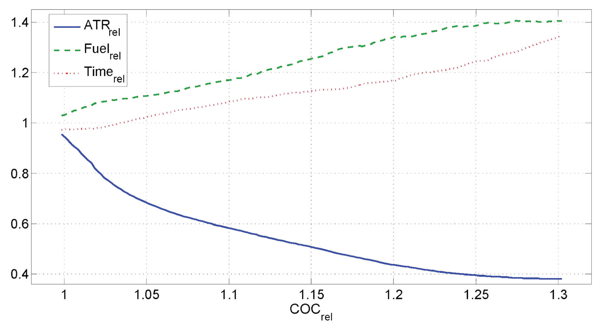
7. Impact of Increasing Fuel Prices on Mitigation Potential and Design Conditions

The considered fuel price directly influences the cost-efficiency of the achievable climate impact mitigation potential ATR${}_{rel,all}$ through COC${}_{rel,all}$. It further has a direct impact on the ICA, $M{a}_{cr}$ frequency distribution and resulting aircraft design conditions that correspond to a selected cost penalty. To quantify the sensitivity of the mitigation potential for the reference aircraft and aircraft design conditions, the fuel price is varied in bounds between 0.9- and three-times the reference fuel price in 2006 (0.595 USD/kg) [59], by using a fuel cost factor (FCF). Even for high fuel price scenarios expected in the future, the climate impact mitigation potential and mitigation efficiency remain favorable (

Table 8. Mitigation potentials and efficiencies at COC${}_{rel,all}$ = 1.1 with corresponding average cruise conditions ($\overline{\mathrm{ICA}}$, $\overline{M{a}_{cr}}$) for selected fuel price factors.

Fuel Cost Factor	ATR Reduction (%)	Mitigation Efficiency	$\overline{\mathbf{ICA}}$ (m)	$\overline{{\mathit{Ma}}_{\mathit{cr}}}$
0.963 (min 2006)	42	4.2	7930	0.718
1.0 (Ref. 2006)	42	4.2	7974	0.717
1.064 (max 2006)	42	4.2	8020	0.717
1.5	40	4.0	8320	0.713
1.67 (average 2012)	40	4.0	8386	0.711
2.0	39	3.9	8520	0.707
2.5	39	3.9	8635	0.700
3.0	38	3.8	8713	0.695

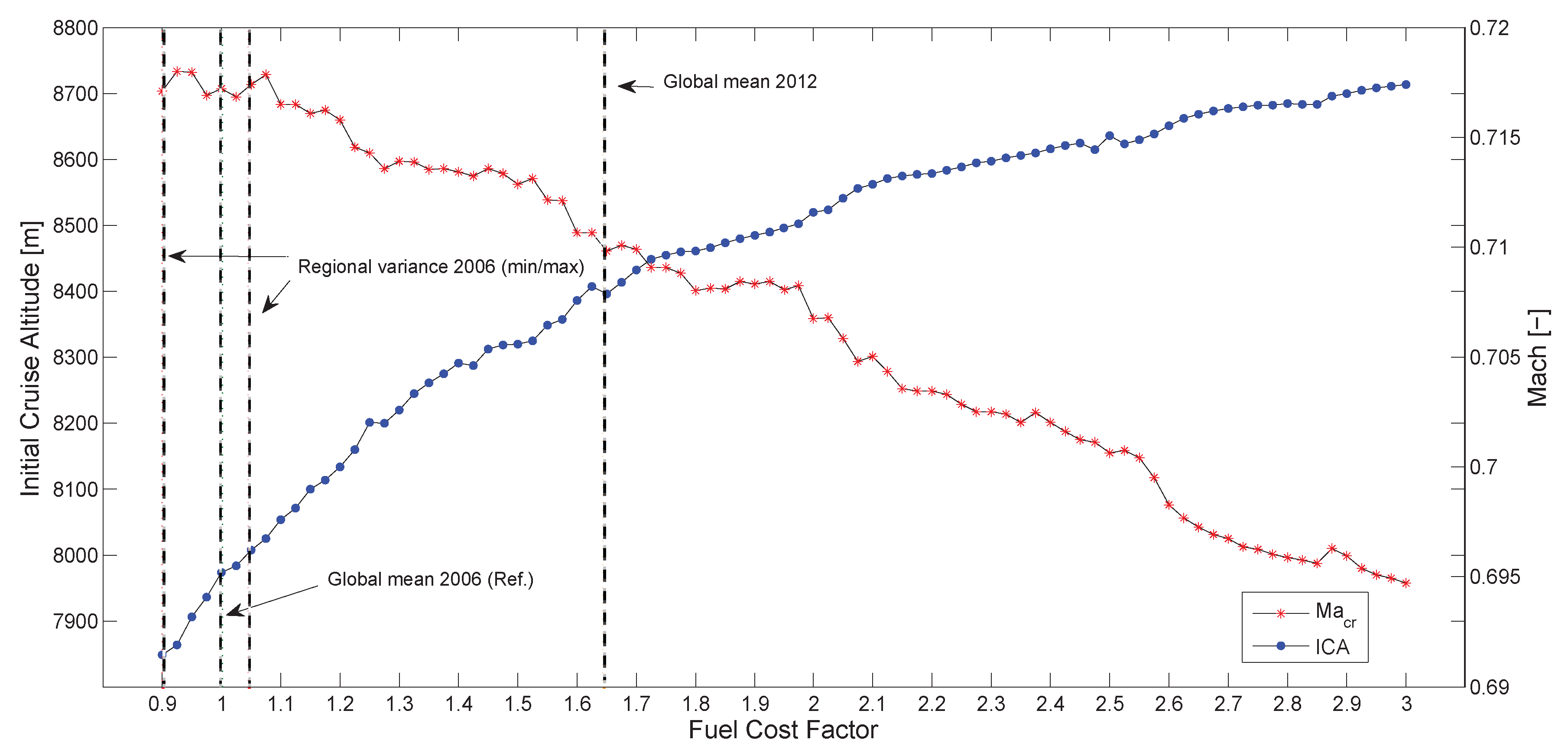
). Analyzing the deviation of ATR${}_{rel}$ at COC${}_{rel,all}$ = 1.1 for a fuel cost factor of three reveals that the mitigation potential only changes by 3.5%. The next step is to analyze the impact of the increasing fuel prices on the design conditions for future aircraft. Figure 14 depicts the evolution of cruise conditions that correspond to the COC${}_{rel,all}$ = 1.1 case as a function of the fuel price. With increasing fuel price, the $\overline{\mathrm{ICA}}$ increases, and $\overline{M{a}_{cr}}$ decreases as increasing ICA and decreasing $M{a}_{cr}$ reduce drag and therewith fuel consumption. Table 8 summarizes the mitigation potentials and efficiencies for selected fuel price factors. The regional fuel price factors in 2006 (+6.4%, −3.7%) [60] are used to verify the robustness of the chosen reference scenario, evaluating the change of the climate impact mitigation potential and corresponding cruise conditions. Analyzing the average cruise conditions found for COC${}_{rel,all}$ = 1.1 shows that $\overline{\mathrm{ICA}}$ varies between 7930 m and 8020 m, while the corresponding $\overline{M{a}_{cr}}$ varies between 0.717 and 0.718. The regional fuel price fluctuations (in 2006) thus have very little impact on the identified climate impact mitigation potential and corresponding cruise conditions applied to actual aircraft design studies.

8. Discussion

The identified mitigation potential depends on the assumptions and sensitivities of the climate response model and operating costs model. To account for the uncertainties concerning the climate response model, we performed a Monte Carlo simulation to consider the uncertainties of different ratios of one climate agent to the total impact [36]. Only trajectories that differ statistically significantly (97.5%) from the reference trajectory are used for further analyses. A considerable part of the uncertainties concerning the climate impact of aviation is hereby taken into account. Remaining uncertainties, which are not covered in the Monte Carlo simulation, are, e.g., the dependency of climate impact on the flight altitude, unresolved atmospheric effects, such as the effects of aerosols on contrails and clouds, and the dependencies of aviation effects on weather situations.

The effects of cruise altitude variations by 2000 ft up and down, respectively, were investigated by the means of complex atmosphere-chemistry models and compared to results obtained with AirClim [36]. All models provide qualitatively the same results, except for methane, where the altitude dependency differs in sign. Grewe and Dahlmann [35] compared the altitude dependency of aviation effects (O${}_3$, H${}_2$O and CiC) to results from Köhler et al. [63] and Rädel and Shine [64] and also found a good qualitative agreement.

There are other non-CO${}_2$ effects not included in this study, as those are much more uncertain. For example, Gettelman and Chen [65] and Righi et al. [28] found effects of aerosols on lower-altitude clouds. They indicate that these effects may be substantial, but also that there are large uncertainties in their quantification.

AirClim provides an annual average response based on simulations over a time horizon of five years with individual weather situations and the related climate impact of aircraft emissions. The calculated climate impact thus implicitly includes weather patterns, but there is no possibility to resolve the response on specific weather situations. AirClim is thus rather applicable for the assessments of long-term mitigation strategies, such as new aircraft concepts, which are designed independently of specific weather situations. In contrast, the assessment of mitigation strategies targeting daily operations, e.g., strategies, such as contrail avoidance or more general avoidance of climate-sensitive regions, rather requires climate impact calculations that consider actual weather situations, such as CoCiP (Contrail Cirrus Prediction Tool) [66] or REACT4C [10].

The identified mitigation potential is based on cash operating costs only, which includes the costs for fuel, crew, maintenance, navigation and landing fees, but does not include costs of ownership (depreciation, interests and insurance). The reduced flight speeds have an impact on the direct operating costs through impacts on the flight schedule and potentially reduced transportation work conducted in the analyzed period. Options to counter this reduction of transport work, such as additional aircraft, are likely to increase the cost of ownership and, thus, DOC. Therefore, the mitigation efficiency will be lower than the values derived in the present study when taking DOC into account.

Passenger acceptance of increased travel times and altered schedules are factors limiting the feasibility and climate impact mitigation potential of the herein analyzed concept. However, additional market-based measures (e.g., analyzed in Scheelhaase et al. [67]) or other climate impact constraints could lead to additional incentives to reduce the climate impact if airlines have to pay for additional climate impact.

Flying at 8000 m thus does not reflect current ATM practice and supposes a flexible ATM for operations with reduced climate impact. In this study, we use meters for analyzing flight altitudes; however, current ATM uses flight level of 1000 ft, which are 305 m. Therefore, our results do represent typically flight levels.

9. Conclusions

We developed a comprehensive simulation and assessment approach with detailed models of various aviation disciplines for the climate impact reduction of aviation in the DLR project CATS. To quantify the climate impact mitigation potential, the developed model workflow was applied for the world fleet of a representative current twin engine long-haul aircraft that is globally operated. Numerous flight profiles were simulated with varying cruise speeds and cruise flight altitudes. For each computed flight trajectory, the changes in ATR and COC are investigated relative to current typical cruise flight conditions obtained from Eurocontrol CFMU data. Based on the resulting ATR and COC changes, Pareto-optimal cruise conditions are derived for each route in the global route network. This shows the route-specific trade-off between the climate impact reduction and the increased COC. Summing the route-specific climate impact mitigation potentials for all routes provides an estimate for the case that all aircraft of the chosen aircraft type are operated globally on flight profiles with reduced climate impact.

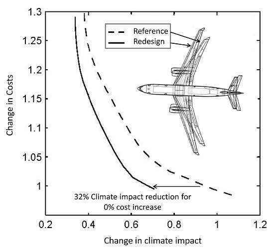
The conducted study shows considerable potential to mitigate climate impact with a small to moderate increase in COC: a 42% ATR reduction for a 10% COC increase or an 11% ATR reduction for a 1% COC increase. The identified mitigation efficiency, which expresses the ratio of achievable ATR reduction for a selected COC increase, is especially favorable at small cost changes.

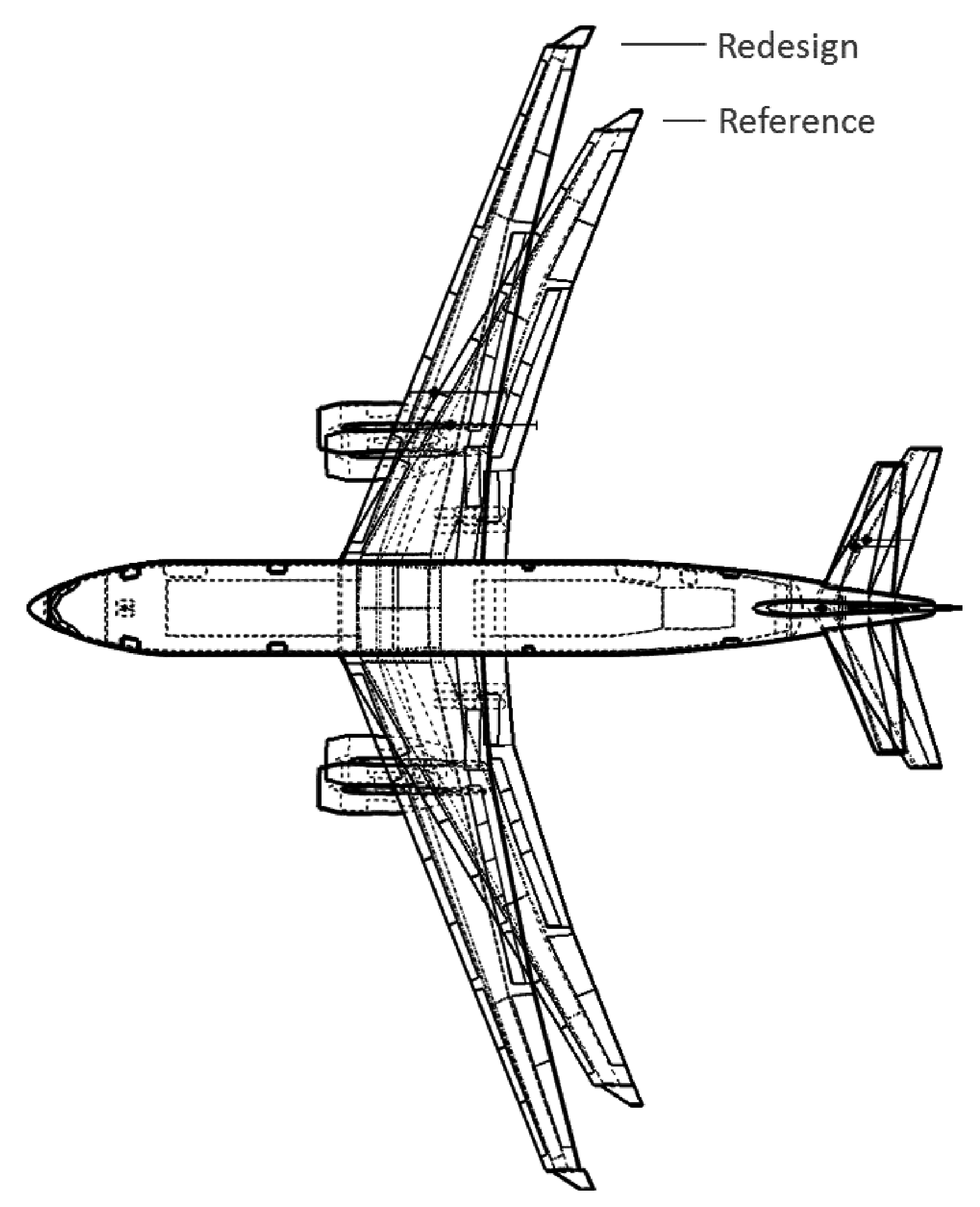
In the second step, average initial cruise conditions ($\overline{\mathrm{ICA}}$, $\overline{M{a}_{cr}}$) are derived for each cost increment on the global Pareto fronts, providing new design conditions for future aircraft that are optimized under cruise conditions with reduced climate impact. Based on this information, the reference aircraft is optimized for cruise conditions corresponding to a COC penalty of 10%. The optimization includes relevant parameters of the wing and tail planes, such as reference wing areas, aspect ratios, LE sweep angles and span-wise twist distributions. To quantify solely the impact of aircraft design changes, the technology level and payload-range capabilities of the reference aircraft are kept constant during the optimization process. The redesigned aircraft shows a fuel-burn improvement of 11% relative to the reference aircraft for the same mission. This fuel improvement allows the reduction of the COC penalty by 4%–5% and an increase of the climate impact mitigation potential by additional 4%–8% depending on the cost penalty. Replacing the entire A330-200 fleet by the redesigned aircraft that is optimized for ICA = 8000 m and $M{a}_{cr}$ = 0.72 allows a climate impact reduction of 32% without an increase of COC. This shows that the combination of lower cruise altitudes and speeds with aircraft design optimization enables the cost-efficient mitigation of aviation-related global warming.

Since the results depend on the fuel price, the present study includes a sensitivity study concerning the impact of increasing fuel prices on the mitigation potential and design conditions. However, the results show that the mitigation potential remains favorable even for high fuel prices expected in future traffic scenarios. The results further showed that the chosen reference scenario has low sensitivity with regional fuel price fluctuations. This provides the robust design conditions for aircraft optimization studies. Nevertheless, the identified mitigation potential depends on the sensitivities of the climate response model and assumptions concerning operating costs. Changing assumptions or new research results in climate impact simulations could change the climate mitigation potential. The results discussed here clearly show the potential of developing a cost-efficient and climate compatible air transport system. The developed simulation workflow provides an ideal basis for future research with increased scope and/or level of fidelity. In this sense, the conducted analyses should be extended to the additional analyses considering further interdependencies between the different air traffic areas. It is for example important to estimate the impact of reduced flight speeds and flight altitudes on airline fleet utilization and related costs, passenger acceptance and air traffic management constraints, such as airspace capacity. Among others, these aspects will be addressed in the DLR research project WeCare (2013–2017).