
Continuation Methods for Nonlinear Flutter

Boreal Racing Shells, Seattle Rowing Center, 1116 West Ewing Street, Seattle, WA 98119, USA
Aerospace 2016, 3(4), 44; https://doi.org/10.3390/aerospace3040044
Submission received: 27 October 2016
/
Revised: 3 December 2016
/
Accepted: 5 December 2016
/
Published: 9 December 2016
(This article belongs to the Special Issue Feature Papers in Aerospace)
Abstract
:Continuation methods are presented that are capable of treating frequency domain flutter equations, including multiple nonlinearities represented by describing functions. A small problem demonstrates how a series of continuation processes can find all limit-cycle oscillations within a specified region with a reasonable degree of confidence. Curves of the limit-cycle amplitude variation with velocity, indicating regions of stability and instability with colors, give a compact view of the nonlinear behavior throughout the flight regime. A continuation technique for reducing limit-cycle amplitudes by adjusting various system parameters is presented. These processes are economical enough to be a routine part of aircraft design and certification.

1. Introduction
In the commercial airplane industry certification that an aircraft is free from flutter instabilities is a major aspect of design and modification, requiring numerous analyses to cover the entire range of flight conditions and design parameters. Because it is impossible to analyze all flight conditions, such as altitude, speed, fuel loading and payload, limited sets of conditions are analyzed, often relying on engineering judgment to pick the important conditions. To do the many analyses required, techniques are typically limited to linear, frequency domain methods, using finite-element models reduced with low-frequency free-vibration modes and linear unsteady aerodynamics from the doublet-lattice method.
Linear flutter equations assume infinitesimally small displacements; nonlinear flutter equations are far more realistic, allowing for limit-cycle oscillation (LCO), self-excited, constant amplitude oscillations that may be harmful or merely ride-quality problems depending on the amplitude. The additional information provided by nonlinear analyses is important to the design of commercial aircraft and should become a routine part of industrial flutter analyses.
Continuation methods, a class of methods for solving parameterized nonlinear equations [1], when applied to linear flutter equations have proven advantageous for covering the range of flight conditions by allowing for continuous variations in parameters, thereby reducing the number of discrete conditions necessary [2]. For example, interpolating mass matrices at several fuel loadings allows tracing the variation of flutter points with fuel loading in a continuous fashion. The success of continuation methods in treating linear flutter equations is due to the fact that in spite of the term linear flutter, the equations are nonlinear in several parameters, but linear in the generalized coordinates (g.c.). Thus, it is a small step to extend continuation methods to treat nonlinear flutter equations, identifying LCOs and tracing the variation of amplitude with parameters, such as velocity.
Single nonlinearities, for example free play or bilinear stiffness in one discrete degree-of-freedom, have been studied for many years [3,4]. A single nonlinearity modeled with a describing function is readily treated with linear flutter techniques, since the generalized coordinates can be normalized to satisfy the amplitude of the single generalized coordinate. Multiple nonlinearities present a conceptually more difficult task because of the need to simultaneously adjust the generalized coordinates so that they and the resulting nonlinearities satisfy the flutter equations. Various schemes have been proposed to address this problem [5,6]. Here, it is shown how a continuation method designed for linear flutter analysis can also be used with multiple nonlinearities with minor modifications. The result is a method that is straightforward, efficient and familiar to flutter engineers.
Following a brief summary of the continuation method presented in [2] and its application to nonlinear flutter equations, a small problem is used to illustrate the search for limit cycle oscillations. With a series of continuation processes, the region of interest is covered with a grid of curves that find almost all LCOs in the region. Because of the sparsity of the grid, an LCO is missed, but is discovered using a continuation method that traces an optimal path toward a limit cycle. Starting from the limit cycles encountered, curves of LCO amplitude versus velocity are traced with continuation. From one of these curves at a specified velocity, the optimal-path continuation method is used to reduce the LCO amplitude by adjusting gains and phases in a simple control system.
2. Continuation Method
Continuation methods solve systems of nonlinear equations that are functions of more variables than equations, at discrete points over a range of the variables while maintaining continuity in the nonlinear functions. Continuity in flutter equations is important because there are always multiple solutions, known as aeroelastic modes, which occasionally become close and difficult to distinguish.
The problem to solve is:
starting from a known solution and varying the independent variables through the desired range. is the dimensionality of the solution: curves (1); surfaces (2); volumes (3), etc. The focus here is on curves: .
The continuation method chosen to solve this is known as a pseudo-arc length method [1] with a minimum-norm corrector. At step j, the next point is predicted using the tangent to the curve and the known solution :
where the stepsize α is an approximate distance along the curve, hence the name pseudo-arc length. Starting with the prediction , the corrector iterates to find the solution using a Newton-like method, computing corrections satisfying:
and setting:
where:
is the Jacobian matrix of derivatives of with respect to . The tangent vector () is characterized by:
where τ is the arc length along the curve.
Equation (3) is an underdetermined linear system that has an infinity of solutions; the smallest such solution can be computed by factoring the transposed Jacobian into an orthogonal matrix times an upper-triangular matrix :
known as a QR factorization. Substituting Equation (7) into Equation (3) yields the minimum-norm solution [7] (p. 300):
Corrector iterations continue using Equations (3)–(8) until suitable convergence criteria are met, for example for some absolute tolerance and relative tolerance :
In preparation for the next predictor step, the tangent is computed from the ( matrix in Equation (7), a by-product of the QR factorization. is an orthogonal matrix spanning the null space of the Jacobian,
An arbitrary vector is projected onto the null space with:
where is the identity and to satisfy Equation (6). If , consists of one column, the projection only determines the sign of the tangent, and a logical choice for the vector to project is the tangent at the previous continuation step to keep the curve tracking in the right direction. In this case, it is not absolutely necessary to do the projection, but it avoids forming (see Section 8) and is necessary for the optimal-path technique (Section 5.6, Section 5.8 and Section 6).
3. Flutter Equations
Treating the flutter equation in the frequency domain has computational advantages over the time domain: the characteristic equation is a system of nonlinear algebraic equations instead of a system of differential equations, which must be integrated at each flight condition. By contrast, the algebraic equations can be solved over a continuous range of flight conditions. The disadvantage is that nonlinearities must be approximated to conform to the harmonic motion assumption, Equation (12).
3.1. Assumed Motion
Linear, frequency domain flutter analyses are based on the assumption that the actual motion of the structure () as a function of time is related to a set of complex generalized coordinates () by:
where Φ is typically a matrix of vibration modes, t is time, is the Laplace variable, ω is the frequency and oscillations are growing, neutral or decaying if the growth factor σ is positive, zero or negative, respectively.
The actual motion in a nonlinear frequency domain flutter analysis does not in general follow this assumption; retaining this assumption results in an a quasi-linear approximation [8]. Describing functions and harmonic balance methods are examples of quasi-linear approximations. Any approximation conforming to these assumptions should work with the methods presented here.
3.2. Equations
Various formulations of the flutter equations have been proposed [9,10,11,12,13]; any of them can be used with the continuation method presented above. A general form of the frequency domain flutter characteristic equations is:
where , , , , and are the () mass, stiffness, gyroscopic, viscous damping, unsteady aerodynamic and control-system matrices, respectively, d is the structural damping coefficient, is the dynamic pressure, is the complex reduced frequency, V is the free-stream velocity, is the free-stream Mach number, a is the sonic velocity and is the complex dynamic matrix.
The related equation:
is a nonlinear eigenvalue problem with solution eigenpair , normalized with the 2-norm of 1.0 and the k-th component real. Contrast this with the generalized-coordinate vector , which is a factor, η times :
This distinction is important when the dynamic matrix is a function of generalized-coordinate amplitudes, particularly when η is small or zero.
3.3. Conversion to Real
The continuation method presented is for real equations and variables; the flutter equations are converted from a set of complex equations to real equations by setting:
so that:
and the 2-norms of the eigenvectors and generalized-coordinate vectors are unchanged:
where is the conjugate transpose.
3.4. Matrix Parameterizations
The matrices in Equation (13) are, in general, not constant; rather, they are assumed to be functions of problem-dependent parameters using various matrix parameterizations. For example, aircraft mass matrices are often parameterized by payload and fuel loading by interpolating matrices at several parameter values. More important for this study, the matrices might be parameterized by generalized-coordinate amplitudes in various ways depending on the matrix and type of nonlinearity. The dynamic matrix is therefore a function of the generalized coordinates and a vector of parameters, such as V, σ, and ω: . Common examples of nonlinearities include structural free play, nonlinear stiffnesses and control systems.
Nonlinear structural elements, such as free play and nonlinear stiffness, can be approximated using describing functions, which conform to the harmonic motion assumption, Equation (12). These stiffness elements are usually modeled with a single degree-of-freedom with no stiffness coupling between it and other degrees-of-freedom [4]. A describing function for bilinear stiffness associated with generalized coordinate j, with stiffness when the displacement amplitude is below δ and when it is above, is:
3.5. Normalization
To make solutions unique, a phase normalization on the generalized coordinates is necessary, for example by constraining the k-th component of to be real:
If in addition η is to be held to a constant value , another equation is added:
Therefore, to trace curves , independent variables must be used if η is allowed to vary, or if it is held constant.
3.6. Continuation Formulations
The independent variables () comprise the variables or , plus enough additional parameters to give an underdetermined system. There are two cases to consider: constant η with variables and variable η with variables.
In what follows, various combinations of velocity, frequency, σ and η are used to demonstrate the solution technique; other parameters are possible, but these three serve to illustrate typical analyses. Each combination of parameters will be named according to which three of these parameters vary; the fourth is implicitly constant. For example, a V-σ-ω analysis traces the variation in σ and ω with velocity, holding η constant, as in a traditional linear flutter analysis, and a V-ω-η analysis traces LCO boundaries, the goal of this study.
3.6.1. Constant η
Solving the flutter equations with the generalized-coordinate norm held to a constant value presents a problem when and possibly numerical difficulties when is small. The vector is known as the trivial solution because even though it is technically a solution, it provides no real information about the behavior of the structure. Yet solutions at are important for determining the stability of the trivial solution, the basis of linear flutter solutions. For this reason, when η is held constant, eigenvectors are used as variables instead of the generalized coordinates. The eigenvector is constrained to unit 2-norm with the addition of an equation like (21): , so there are equations, and three more parameters are necessary for independent variables.
For the demonstration parameters, the equations are:
where is row of the order identity matrix.
3.6.2. Variable η
If η is allowed to vary, the additional normalization Equation (21) is not used, so there are equations: Equation (17) plus the phase normalization (Equation (20)),
and two of the three parameters () are needed.
Two combinations of the three parameters will be of interest, σ-ω-η at constant velocity (used to search for ) with:
and V-ω-η at constant σ (used to trace LCO boundaries):
If the first step in either of these processes starts from a known solution at with:
a modification in the tangent calculation is necessary, because the Jacobian and its null space vectors are then:
The third column of gives the desired greatest increase in η, so the first predicted solution for the σ-ω-η process is:
In addition, an equation should be added to prevent converging to the trivial solution (),
where is the 2-norm of the predicted . For the first step, .
4. Demonstration Problem
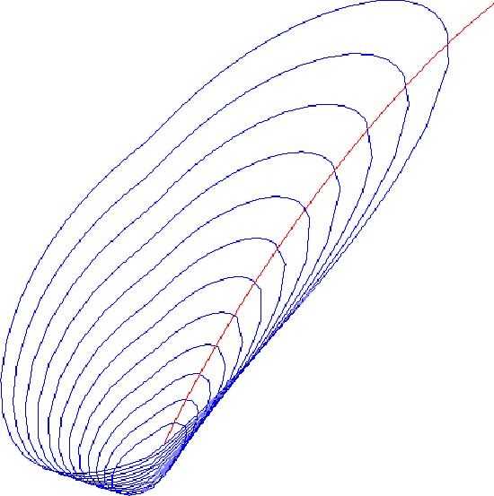
A small, well-known problem illustrates the use of these continuation processes. The model is Example 9-1 in [14], implemented as Example HA145B in finite-element program MSC-NASTRAN [13], with a generalized-coordinate basis of free-vibration modes and doublet-lattice aerodynamics. Bilinear nonlinearities are applied to the first four diagonals of the (diagonal) stiffness matrix using the describing function of Equation (19) with , (hardening) for diagonals 1 and 2, (softening) for diagonal 3 and (softening) for diagonal 4. Figure 1 shows the model wing planform and unsteady aerodynamic grid.
5. Searching for Limit Cycle Oscillations
Limit cycle oscillation is a condition where the structure is oscillating with an amplitude that is neither growing nor decaying; it is in dynamic equilibrium and . On the other hand, is a static equilibrium with stability determined by the sign of σ. The goal then is to find all points within the region of interest where .
The strategy is to find several points where using the formulations of Section 3.6.1 and Section 3.6.2, then use these points to start V-ω-η processes to trace the variation of LCO amplitude with velocity.
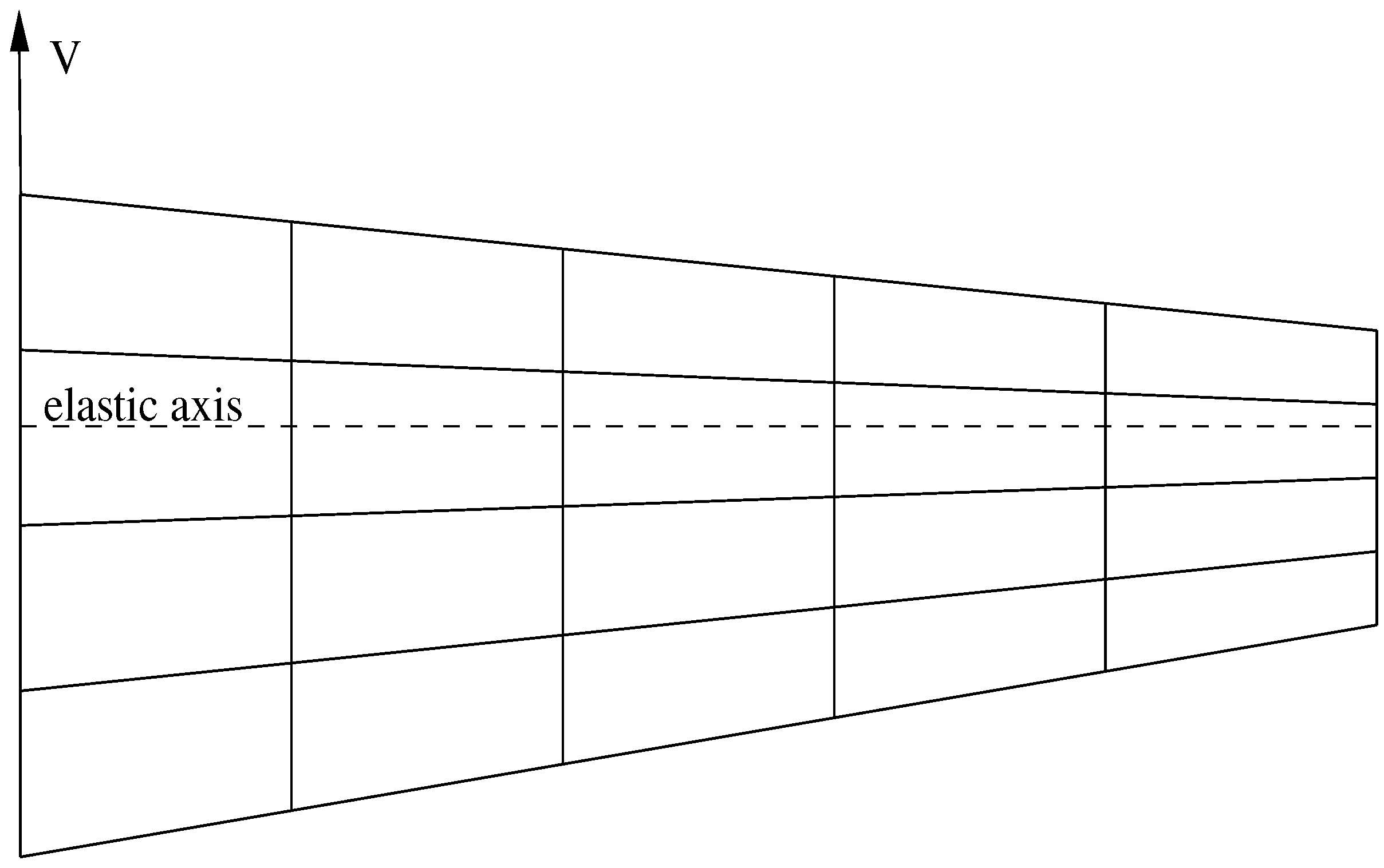
An example of the results of an LCO analysis is shown in Figure 2 where η is plotted against velocity normalized with respect to the maximum velocity of interest, . Ordinarily, η would not be the plot variable of choice; instead, one or more of the nonlinear generalized-coordinate amplitudes would be plotted against velocity, but this choice is problem dependent, so η is used for generality. Of the two curves in Figure 2, only the bottom one extends to , so it is the only one that would be detected in a linear flutter analysis. Detecting the upper curve is why the processes of Section 3.6.1 and Section 3.6.2 are necessary.
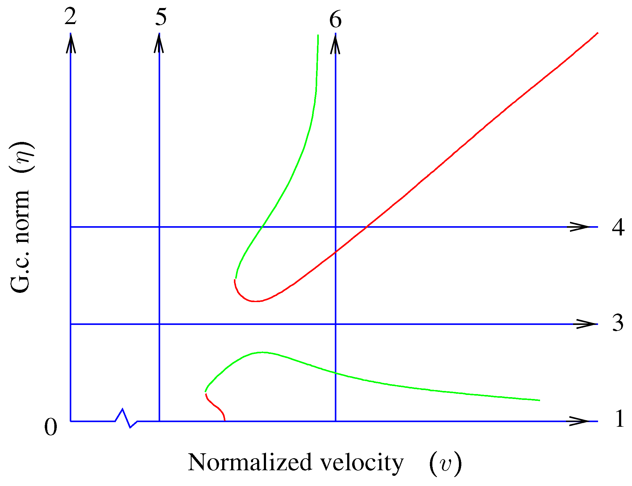
A systematic method for this search is to cover the range with a grid of V-σ-ω and σ-ω-η processes, any of which might encounter points. Figure 3 shows a minimal grid of six lines where horizontal lines are V-σ-ω processes (numbered 1, 3 and 4), and vertical lines are σ-ω-η processes (numbered 2, 5 and 6). Arrows indicate the direction of the continuation processes. Each of these lines represents one or more modes chosen to cover the frequency range of interest.
This set of processes is started from a free-vibration solution, at the origin of Figure 3 (Point 0), with . Two processes are started from this free-vibration solution: Process 1, a V-σ-ω process along the v axis, and Process 2, a σ-ω-η process along the η axis. The remaining vertical and horizontal grid lines are started from these two by interpolating to the desired points.
5.1. Point 0: Free-Vibration
At , the aerodynamic term drops out, and with , is zero for the purposes of evaluating the dynamic matrix . The problem to be solved then is in general the complex nonlinear eigenvalue problem, Equation (14). Under certain conditions, Equation (14) reduces to a polynomial eigenvalue problem [15], or to a generalized eigenvalue problem [16]. For example, in the absence of controls equations, viscous and structural damping and gyroscopics, the eigenvalue problem reduces to the real, generalized eigenvalue problem:
Otherwise, it is usually necessary to resort to nonlinear eigenvalue solution techniques [15].
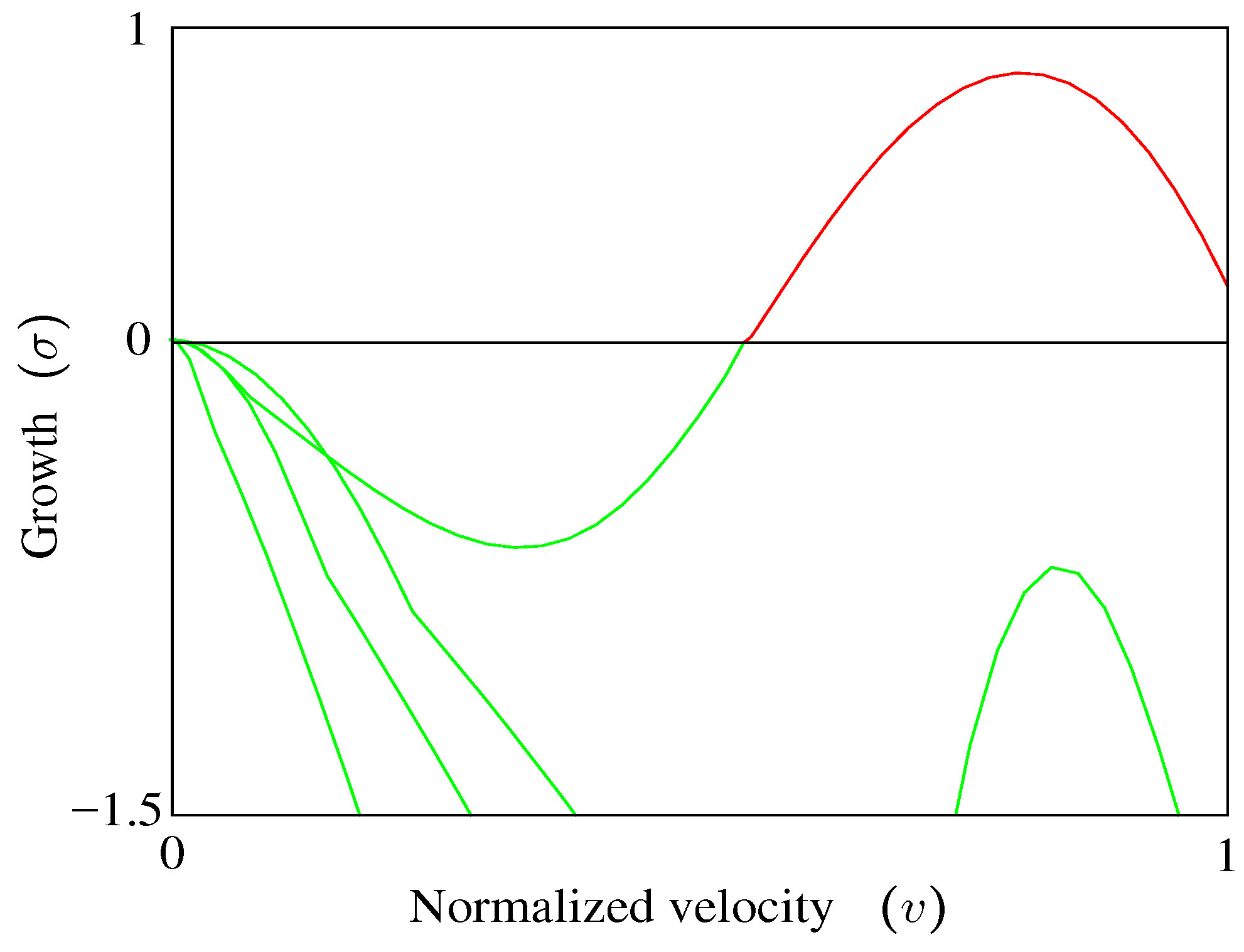
5.2. Process 1: V-σ-ω with
A continuation process along the horizontal axis of Figure 2 is a V-σ-ω process at , solving Equation (22), starting with select eigenvalues and eigenvectors from the free-vibration solution. This is equivalent to a linear flutter solution. Figure 4 shows results for the first four lowest frequency modes with green indicating a stable equilibrium and red unstable.
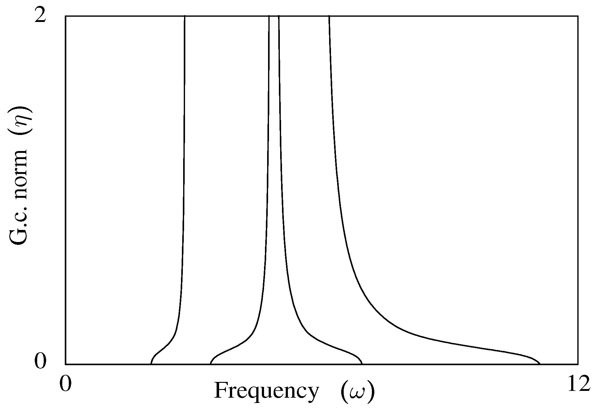
5.3. Process 2: σ-ω-η at
In a σ-ω-η process η is allowed to vary; velocity is held constant; and the Equations are (23) and (23a). With , this process corresponds to the vertical axis of Figure 2. Start points for this process are again select eigenvalues and eigenvectors from the free-vibration solution. At zero velocity, the aerodynamic term drops out, and without viscous or structural damping, for each vibration mode. Only the frequency changes with increasing η, as shown in Figure 5.
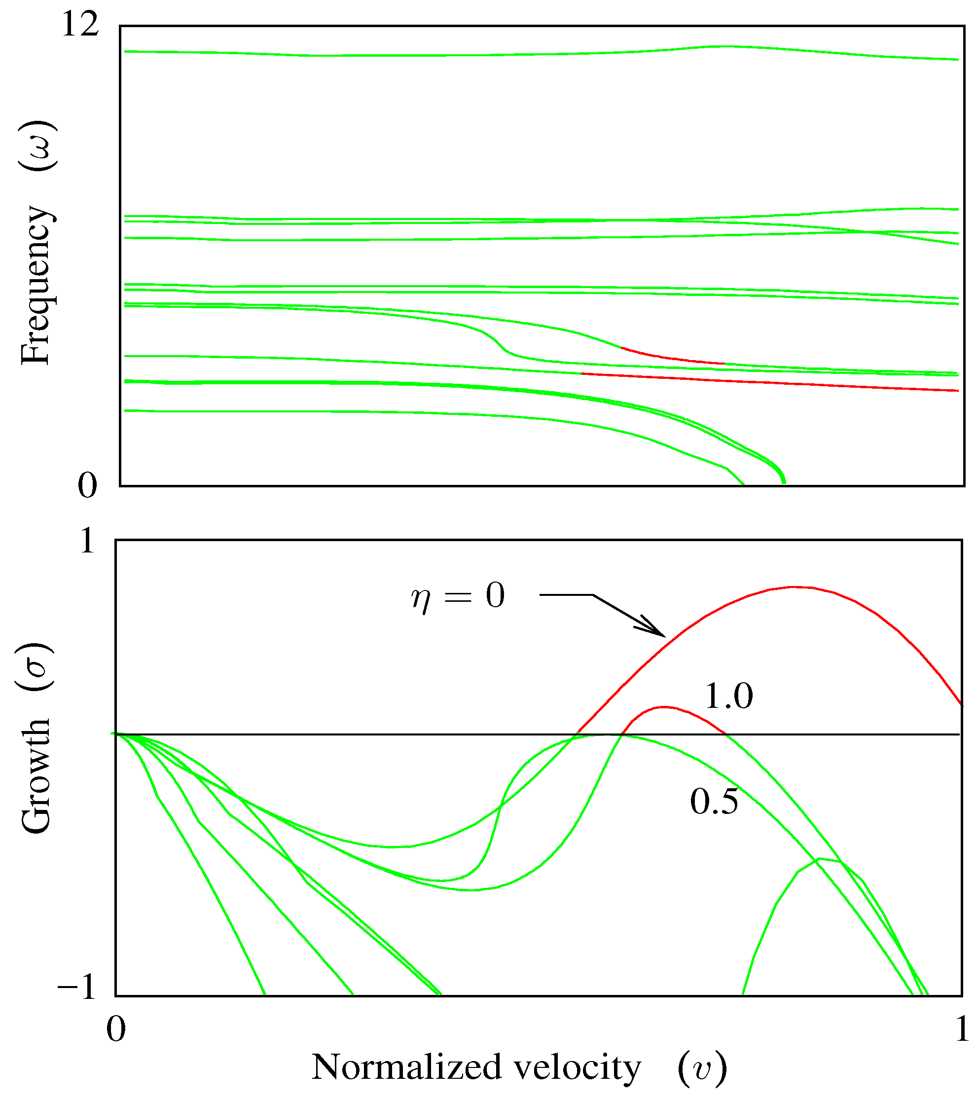
5.4. Processes 3 and 4: V-σ-ω
Horizontal lines 3 and 4 in Figure 3 are V-σ-ω processes starting from Process 2 interpolated to the desired values of η. Figure 6 shows the result of these processes; as before, green indicates stability (negative σ), and red indicates instability. Three levels of η are highlighted for the only mode that crosses . These crossings will be used in the V-ω-η processes of Section 3.6.2 to trace LCO boundaries.
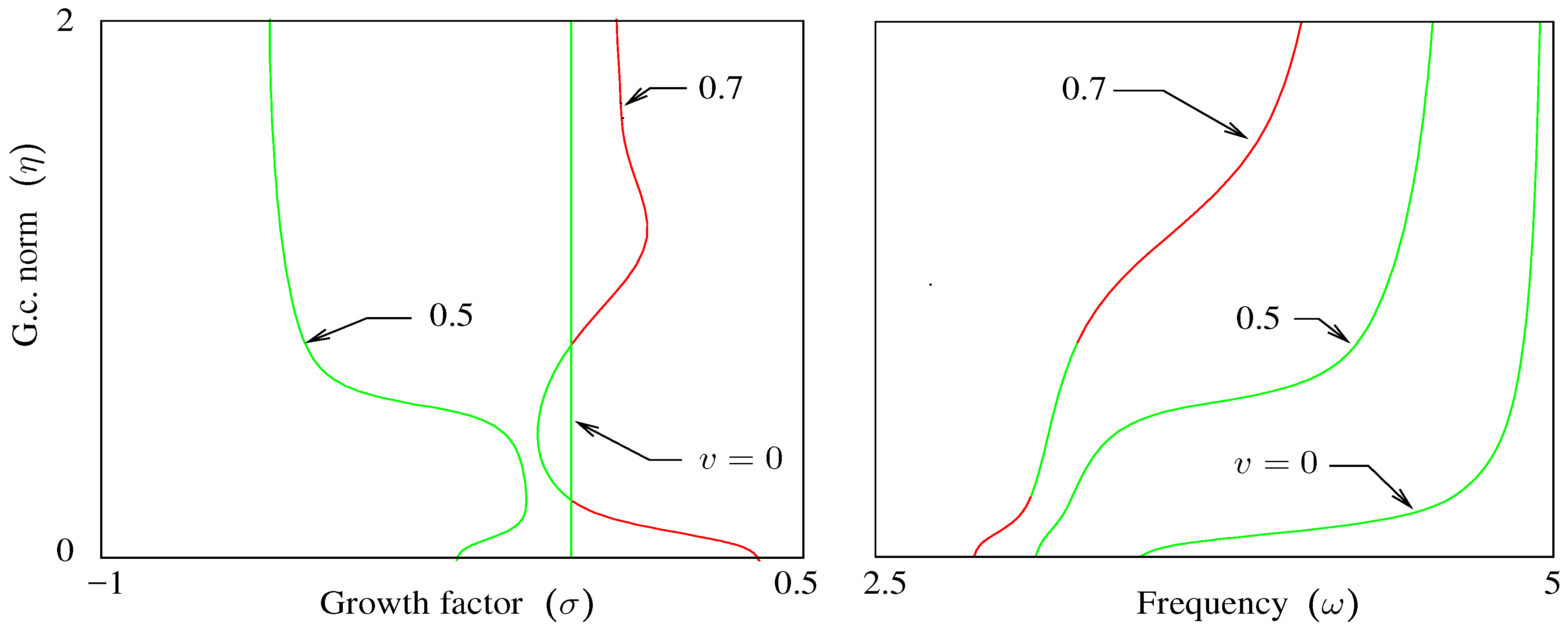
5.5. Processes 5 and 6: σ-ω-η
σ-ω-η Processes 5 and 6 are started by interpolating the curves for each mode traced in Process 1 to the desired velocity. Figure 7 shows σ versus η at three velocities; for clarity, only one of the four modes traced in Process 1 is shown, the only one that encounters LCO.
5.6. Stability of Equilibria
At an LCO, if a small perturbation in the generalized coordinates decreases η and η continues to decrease with time, or if the perturbation increases η and η continues to increase with time, the equilibrium is unstable. On the other hand, if after the perturbation, the generalized coordinates return to the LCO amplitudes, the equilibrium is said to be stable. Mathematically, this means that stability is determined by the sign of the derivative of σ with respect to η: positive indicates instability, and negative indicates stability. This derivative can be computed from the components of the tangent vector corresponding to σ and , recalling Equation (6),
where τ again is the arc length along the curve. These tangent components are available at every step of a σ-ω-η process, but this information is only relevant at . More important is the stability of each point of LCO boundaries, created with V-ω-η processes and Equation (23b). That Jacobian then must be converted to the Jacobian of Equation (23a) by replacing the first column with ,
where:
It is not necessary to actually make this replacement and re-factorize the Jacobian; only the vectors and are of interest because with them, the QR factorization of the transposed Jacobian can be updated [7] (p. 334):
Updating the factorization requires a small fraction of the work required to factorize the Jacobian. From the updated Jacobian, the tangent used in Equation (29) is computed by projecting onto the updated null space with Equation (11):
As η increases or decreases from an unstable equilibrium, the next equilibrium may be stable or unstable. Often, an unstable equilibrium will be followed by a stable one; Figure 7 shows why this is true when the equilibriums are associated with the same aeroelastic mode. That this is not always true will be shown in Section 5.8, where an LCO is discovered associated with a different aeroelastic mode.
5.7. Limit Cycles: V-ω-η Analysis at
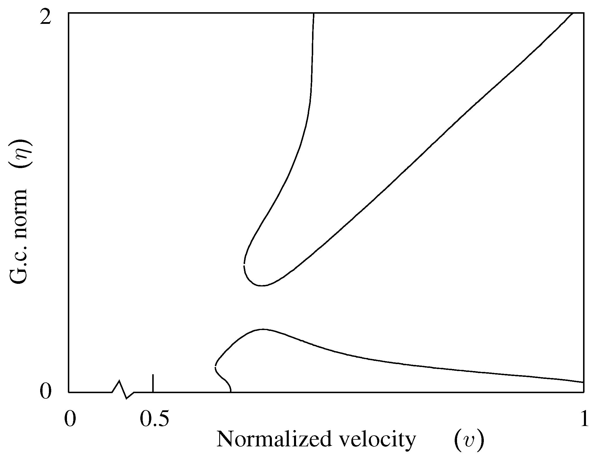
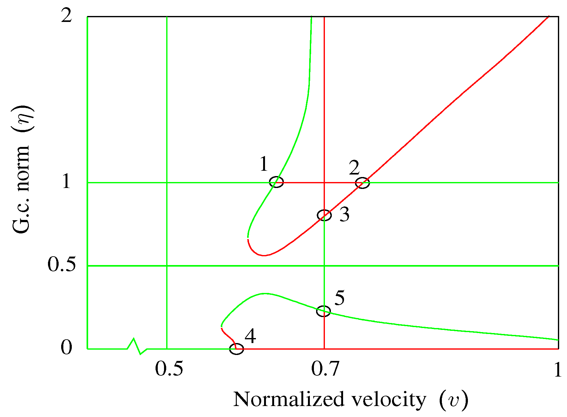
Among the six sets of continuation curves in Figure 6 and Figure 7, there are five points where , at the intersection of the green and red line segments in Figure 8.
These points can be used to start V-ω-η processes, the goal in this exercise, shown as dotted curves in Figure 8. The upper dotted curve could be started from Point 1, 2 or 3; either start point will trace the same curve. Likewise, the lower dotted curve could be started from Point 4 or 5.
5.8. Optimal Path: V-σ-ω-η Analysis
Two of the grid lines in Figure 3 do not cross the axis ( in Figure 6 and in Figure 7), but come close. If all four parameters were allowed to vary instead of holding one fixed and varying the other three, those two continuation processes might have also found limit cycle points. A continuation process where the number of unknowns is greater than the number of equations plus one requires only a minor modification of the continuation process and is in a sense an optimization procedure.
The idea is to allow any number of independent variables greater than the number of equations (m) and to trace a special curve on the surface (or volume, or higher-dimension manifold): the shortest path toward some goal, for example maximizing or minimizing some parameter β. The key to tracing this curve is the tangent to the curve, computed by projecting the vector:
onto the null space of the Jacobian (Equation (11)). Aside from this modification, the continuation process is unchanged.
Here, the goal is , a limit-cycle oscillation, and the equations are:
Assuming the start point is at a negative σ, the tangent vector is computed by projecting:
onto the null space of the Jacobian (Equation (11)).
Figure 9 and Figure 10 show the result of such a process, starting at a mode in Figure 4 that peaks around and and continuing until is encountered.
Then, starting from the point where this curve meets , a V-ω-η process traces a limit-cycle curve shown in Figure 11.
The complete set of LCO curves, with stable and unstable LCO again shown in green and red, is shown in Figure 12.
Note that at in Figure 12, as η increases from the unstable (static) equilibrium at zero, the next equilibrium encountered is also unstable, followed by two stable equilibriums and finally an unstable LCO. A σ-ω-η process would show continuity in two different modes, a three-Hertz mode and a 10-Hertz mode, and each of these would have the usual pattern of stable followed by unstable and vice versa.
6. Decreasing LCO Amplitudes
It is often desirable to reduce the amplitude of limit cycles, whether to avoid structural damage or to improve ride quality. Sometimes, this can be done with structural changes, such as reducing free play or increasing damping; in other situations, such changes might be impractical, and it may be necessary to resort to control systems. In either case, the technique of Section 5.8 can be used to decrease the amplitude of a generalized coordinate undergoing LCO.
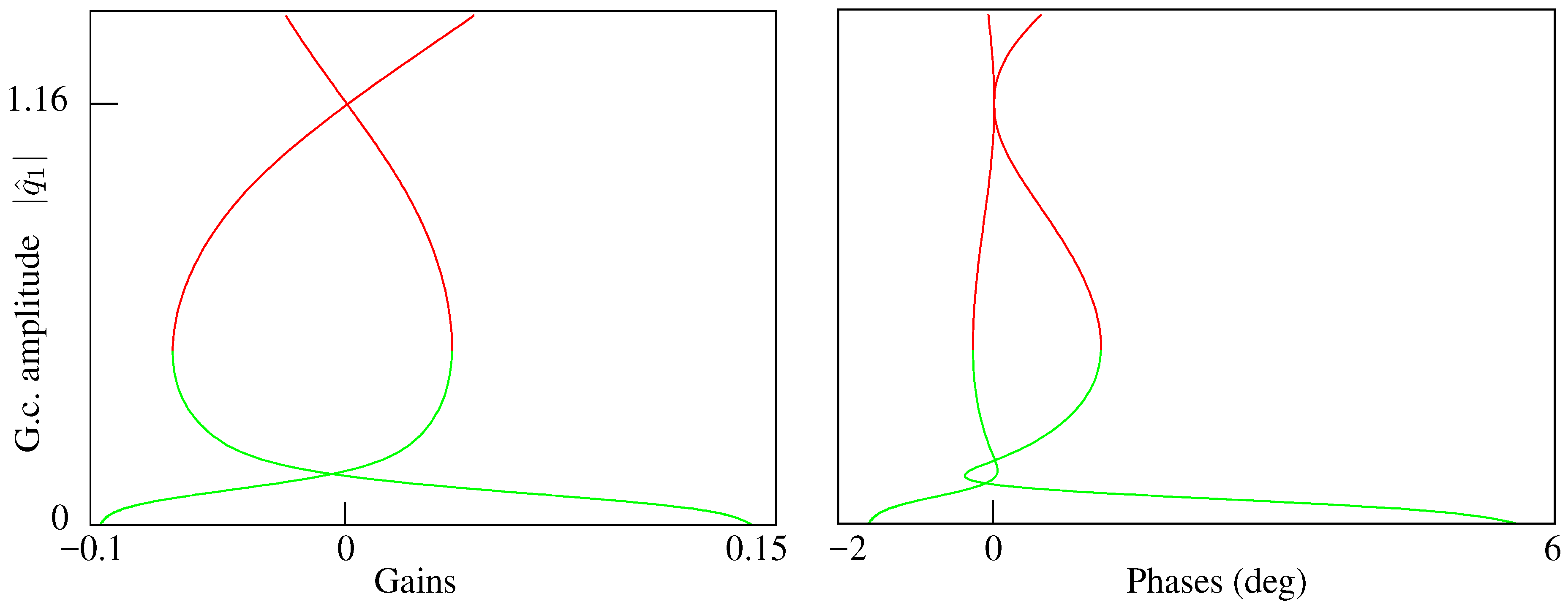
For example, including a simple control system (matrix in Equation (13)) can be used to reduce the amplitude of generalized coordinate 1 in the unstable LCO at normalized velocity 0.8 in Figure 12. Details of the control system are unimportant, as it is just for illustration; it simply feeds back displacement in generalized coordinates 1 and 2 to add stiffness to these coordinates with two complex gains: and . The equation to be solved is as before, Equation (23), with , but now with three more unknowns than equations:
A projection vector pointing towards decreasing is:
Beginning at on the upper curve in Figure 12, where and , the projection vector guides the solution toward , as shown in Figure 13. The stability of the LCO at each point on the curves is computed as in Section 5.6.
7. Bifurcation
When tracing a curve with a continuation method, it is possible to encounter a bifurcation, where two curves cross [1,17]. Other characteristics of a bifurcation, useful in detecting their presence, are a rank-deficient Jacobian matrix and a change in the sign of the determinant of the Jacobian matrix augmented with the tangent vector. It can be shown [1] that a change in the sign of:
indicates that a bifurcation has been passed. A method for computing μ is shown in Section 8 that is economical enough that it could (and should) be done at every step.
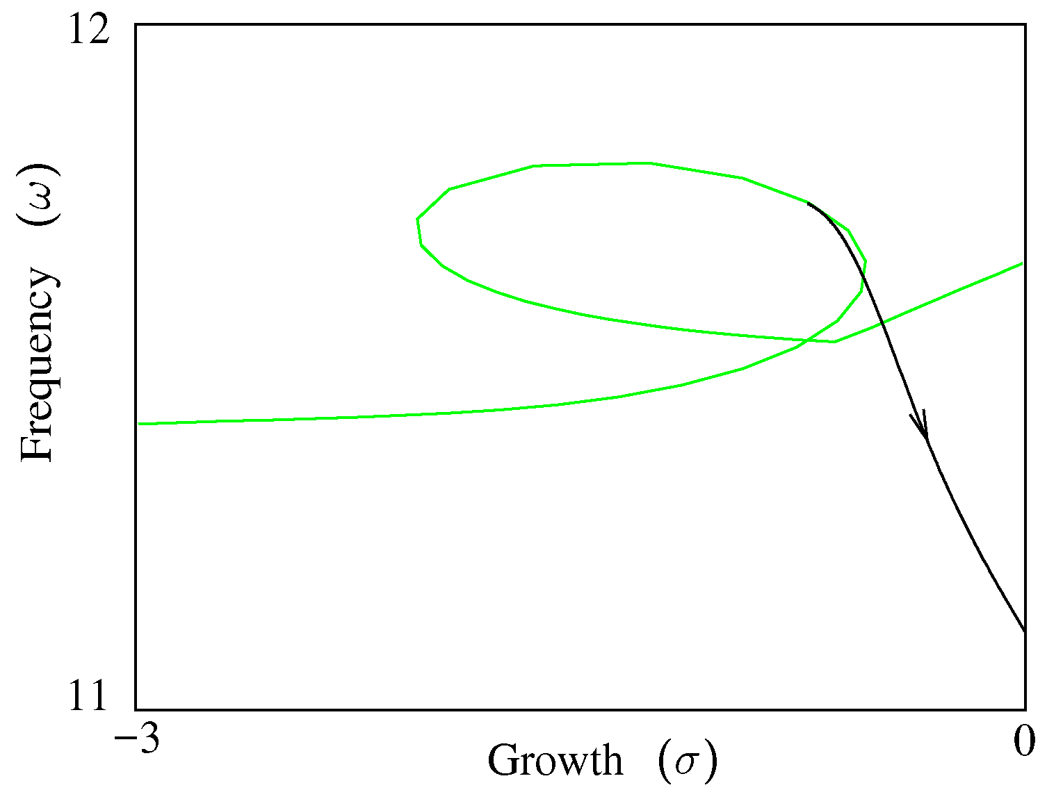
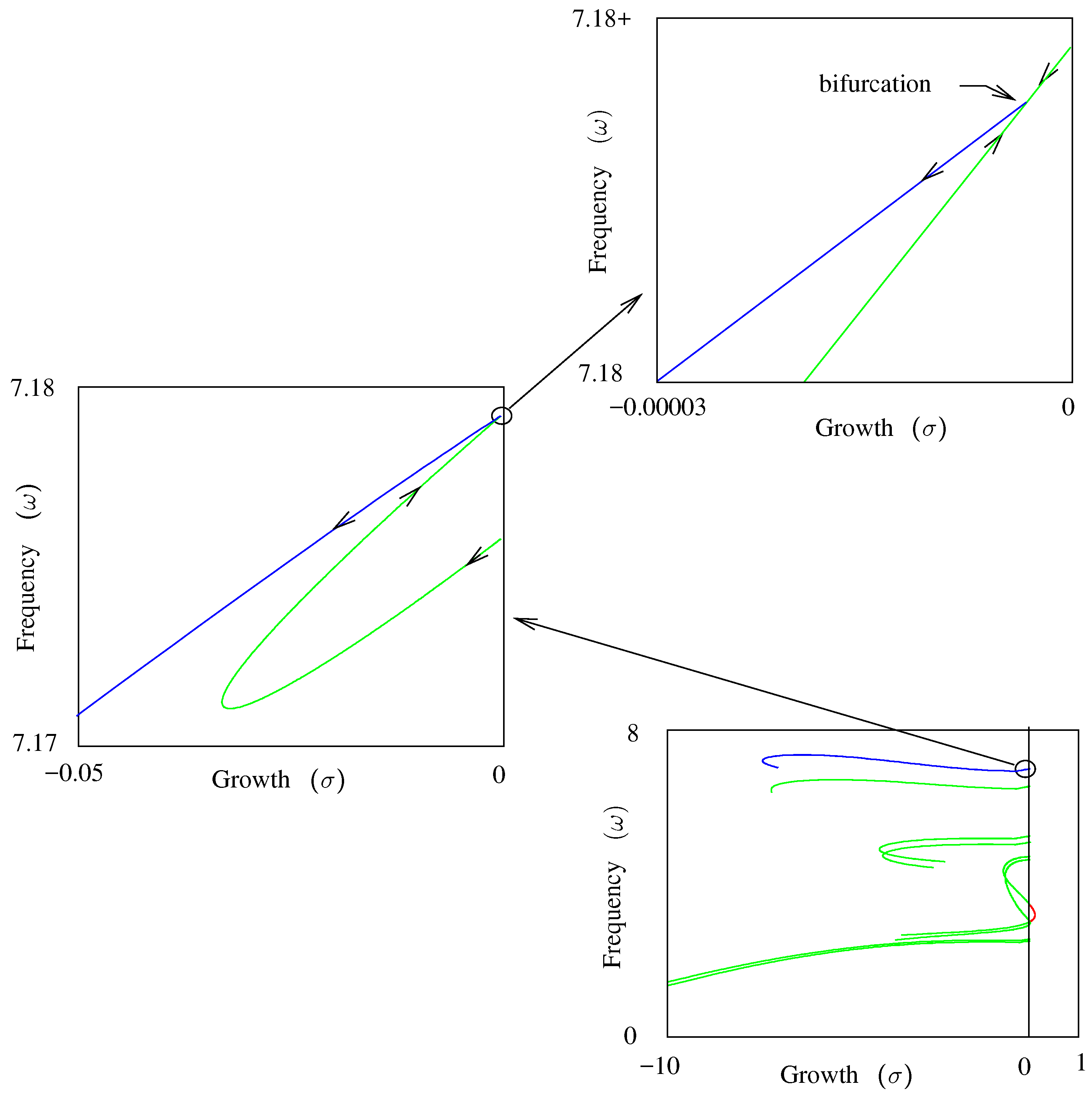
One of the curves in the V-σ-ω process shown in Figure 6 encounters a bifurcation, although it is not evident at that scale. When plotted σ versus ω with an expanded scale, the bifurcation becomes more evident, as shown in Figure 14. Arrows indicate the direction of the positive determinant. Had the bifurcation not been detected, the process would have tracked only the green curve. Detecting the bifurcation and computing the bifurcation tangent allows the blue curve to be traced.
A brief summary of the steps necessary to trace the bifurcation branch is given here; for more detail, see [1,17].
Branching from the bifurcation requires the tangent to the branch curve. For a simple bifurcation at , detected by a change in the sign of , the Jacobian will have one rank deficiency, and the matrix has two columns, some combination of which gives the branch tangent; and another combination continues the original curve.
A singular value decomposition (SVD) [7] (p. 76) of the Jacobian at ,
reveals the rank and is necessary for branching from the bifurcation. The last column of () and the last two columns of ( and ) are left and right null vectors of the Jacobian, and the two tangents emanating from the bifurcation are combinations of these:
where:
One of these tangents is aligned with the original curve, the other with the bifurcation curve. Comparing with the previous tangent determines which is the primary tangent () and the bifurcation tangent ():
8. Programming Considerations
Much of the computational effort in the continuation method is in the factorization of the Jacobian matrix in Equation (7), where QR factorizations are used to solve the underdetermined system. Some continuation methods [1,18] add an equation in the corrector phase to constrain corrections, for example to hold one of the variables constant, creating a square set of linear equations that can be solved using an LU factorization instead of QR. Theoretically, LU is faster than QR; but QR is more stable, and modern computer architectures eliminate the speed advantage [7] (p. 299). QR is also necessary for the optimal-path technique of Section 5.8.
The linear algebra library LAPACK [19] provides several variants of QR factorizations; the preferred routine for efficiency and stability is SGEQP3 [16] (Section 2.4.2.3). None of the QR routines in LAPACK return the and matrices directly; instead, all of the information to create them is returned in the input matrix and a separate array named TAU. The matrix is contained in the upper triangle of the input matrix, and subroutine STRSM solves a set of equations with it. Subroutine SORMQR is provided to multiply or by a vector.
Projecting a vector onto the null space of the Jacobian can be done in LAPACK without actually forming the matrix with two calls to subroutine SORMQR:
that is, call SORMQR to multiply the vector by , zero the first m elements of the result, then call it again to multiply by .
Updating the QR factorization to determine stability with Equation (32) can be done efficiently with the qrupdate package available at [20].
Evaluating the determinant in Equation (39) is simplified by recognizing that the tangent came from the QR factorization, that the determinant of an orthogonal matrix is and that the determinant of a triangular matrix is the product of the diagonals. Furthermore, the tangent and the QR factorization of the Jacobian it was computed from are available from the last corrector iteration, so the desired determinant is:
where k is the number of non-zero elements in the TAU array [21] for LAPACK QR routines, and l is if is positive, −1 otherwise.
Derivatives are an essential part of continuation methods. Accurate derivatives of parameters and matrices with respect to the independent variables are necessary for computing the Jacobian matrix that is used both to iterate to solutions and predict the next solution. Deriving formulas for complicated expressions like Equation (19) can be tedious and error-prone. A technique that eliminates the need for closed expressions for the derivatives and can reduce coding errors is automatic differentiation [22]. This programming technique gives exact derivatives at a cost on the order of evaluating the function itself, in contrast with difference approximations, which are not exact and much more expensive to compute. The autodiff.org [23] website is devoted to automatic differentiation resources.
9. Conclusions
A continuation method capable of treating frequency domain flutter equations with multiple nonlinearities approximated with describing functions has been developed. With it, a set of continuation processes can find with reasonable certainty all limit-cycle oscillations within a desired flight envelope, tracing curves of limit-cycle amplitude versus velocity and indicating stability with colors.
With a small modification to the continuation method, curves can be traced taking an optimal path with respect to any number of parameters toward some goal. This technique was used to seek out a limit cycle that was missed and to reduce limit-cycle amplitudes by adjusting control-system parameters.
Tracing curves with continuation methods, it is always possible to encounter bifurcation. Detecting bifurcation is inexpensive enough that it can be done at every step when tracing a curve; missing a bifurcation risks missing an important curve. When a bifurcation is detected, a straightforward calculation gives the two tangents, which are then used to start continuation processes to trace each curve from the bifurcation.
Conflicts of Interest
The author declares no conflict of interest.
Nomenclature
| a | sonic velocity |
| , | complex and equivalent real dynamic matrices (Equations (13) and (16)) |
| d | structural damping coefficient |
| vector of n real, nonlinear equations | |
| Jacobian matrix of partial derivatives (Equation (5)) | |
| , | row i and column j of matrix |
| , , , | mass, stiffness, gyroscopic, viscous damping, |
| , , | unsteady aero and control-system matrices (Equation (13)) |
| M | , Mach number |
| the number of generalized coordinates | |
| p | , complex reduced frequency |
| 2-norm of vector | |
| q | , dynamic pressure |
| , | complex and equivalent real generalized coordinates (g.c.) (Equations (12) and (16)) |
| , | QR factors of the transposed Jacobian (Equation (7)) |
| , | the real n-vectors and m by n matrices |
| real and imaginary parts of a complex variable | |
| r, γ, δ | bilinear stiffness describing-function variables (Equation (19)) |
| s | Laplace variable |
| tangent vector | |
| V | velocity (true airspeed) |
| maximum velocity of interest (true airspeed) | |
| v | normalized velocity |
| projection vector (Equation (11)) | |
| independent variables | |
| iteration at the continuation step (Equation (2)) | |
| element of vector | |
| complex and equivalent real eigenvector | |
| motion of points of the structure (Equation (12)) | |
| η | 2-norm of the generalized coordinates (Equation (15)) |
| ω | oscillation frequency (imaginary part of the Laplace variable) |
| Φ | transformation from generalized to physical coordinates |
| ρ | fluid density |
| σ | growth factor (real part of the Laplace variable) |
| τ | arc length along a curve |
| transpose |
References
- Allgower, E.L.; Georg, K. Numerical Continuation Methods: An Introduction; Springer Series in Computational Mathematics; Springer: Berlin, Germany, 1990; Volume 13. [Google Scholar]
- Meyer, E.E. Unified Approach to Flutter Equations. AIAA J. 2014, 52, 627–633. [Google Scholar] [CrossRef]
- Shen, S.F. An Approximate Analysis of Nonlinear Flutter Problems. J. Aerosp. Sci. 1959, 26, 25–32. [Google Scholar] [CrossRef]
- Gordon, J.T.; Meyer, E.E.; Minogue, R.L. Nonlinear Stability Analysis of Control Surface Flutter with Freeplay Effects. J. Aircr. 2008, 45, 1904–1916. [Google Scholar] [CrossRef]
- Lee, C.L. An Iterative Procedure for Nonlinear Flutter Analysis. AIAA J. 1986, 24, 833–840. [Google Scholar] [CrossRef]
- Breitbach, E.J. Flutter Analysis of an Airplane with Multiple Structural Nonlinearities in the Control System; NASA Langley Research Center: Hampton, VA, USA, 1980.
- Golub, G.H.; Van Loan, C.F. Matrix Computations, 4th ed.; The Johns Hopkins University Press: Baltimore, MD, USA, 2013. [Google Scholar]
- Gelb, A.; Vander Velde, W.E. Multiple-Input Describing Functions and Nonlinear System Design; McGraw-Hill: New York, NY, USA, 1968. [Google Scholar]
- Hassig, H.J. An Approximate True Damping Solution of the Flutter Equation by Determinant Iteration. J. Aircr. 1971, 8, 885–889. [Google Scholar] [CrossRef]
- Chen, P.C. Damping Perturbation Method for Flutter Solution: The g-Method. AIAA J. 2000, 38, 1519–1524. [Google Scholar] [CrossRef]
- Van Zyl, L.H.; Maserumule, M.S. Divergence and the p-k Flutter Equation. J. Aircr. 2001, 38, 584–586. [Google Scholar] [CrossRef]
- Edwards, J.W.; Wieseman, C.D. Flutter and Divergence Analysis Using the Generalized Aeroelastic Analysis Method. J. Aircr. 2008, 45, 906–915. [Google Scholar] [CrossRef]
- Rodden, W.P. MSC/NASTRAN Handbook for Aeroelastic Analysis; The MacNeal-Schwendler Corporation: Santa Ana, CA, USA, 2009; pp. 357–372. [Google Scholar]
- Bisplinghoff, R.L.; Ashley, H.; Halfman, R.L. Aeroelasticity; Addison-Wesley: Reading, MA, USA, 1955. [Google Scholar]
- Ruhe, A. Algorithms for the Nonlinear Eigenvalue Problem. SIAM J. Numer. Anal. 1973, 10, 674–689. [Google Scholar] [CrossRef]
- Anderson, E.; Bai, Z.; Bischof, C.; Blackford, S.; Dongarra, J.; Du Croz, J.; Greenbaum, A.; Hammarling, S.; McKenney, A.; Sorensen, D. LAPACK Users’ Guide, 3rd ed.; Siam: Philadelphia, PA, USA, 1999. [Google Scholar]
- Meyer, E.E. Continuation and Bifurcation in Linear Flutter Equations. AIAA J. 2015, 53, 3113–3116. [Google Scholar] [CrossRef]
- Rheinboldt, W.C.; Burkardt, J.V. A Locally Parameterized Continuation Process. ACM Trans. Math. Softw. 1983, 9, 215–235. [Google Scholar] [CrossRef]
- LAPACK—Linear Algebra PACKage. Available online: https://www.netlib.org/lapack (accessed on 18 June 2016).
- Hajek, J. Qrupdate. Available online: https://sourceforge.net/projects/qrupdate/ (accessed on 2 September 2016).
- Langou, J. Determinant in QR factorization. Available online: http://icl.cs.utk.edu/lapack-forum/viewtopic.php?f=2&t=1741 (accessed on 14 May 2011).
- Griewank, A.; Walther, A. Evaluating Derivatives: Principles and Techniques of Algorithmic Differentiation, 2nd ed.; Siam: Philadelphia, PA, USA, 2008. [Google Scholar]
- Community Portal for Automatic Differentiation. Available online: http://www.autodiff.org (accessed on 2 September 2016).
Figure 1.
HA145B planform, elastic axis (dashed line), and doublet-lattice grid.

Figure 2.
Typical limit-cycle oscillation (LCO) plot from a V-ω-η analysis.

Figure 3.
Grid (blue) for finding limit cycles. Green means stable, red means unstable.

Figure 4.
Process 1: V-σ-ω analysis with (Green means stable, red means unstable).

Figure 5.
Process 2: σ-ω-η analysis with .

Figure 6.
Processes 1, 3 and 4: V-σ-ω at three η (Green means stable, red means unstable).

Figure 7.
Processes 2, 5 and 6: σ-ω-η at 3 normalized velocities (Green means stable, red means unstable).
Figure 7.
Processes 2, 5 and 6: σ-ω-η at 3 normalized velocities (Green means stable, red means unstable).

Figure 8.
Five start points for LCO curves (Green means stable, red means unstable).

Figure 9.
Optimal path starting from V-σ-ω at (black curve with arrow indicating tracking direction) (Green means stable, red means unstable).
Figure 9.
Optimal path starting from V-σ-ω at (black curve with arrow indicating tracking direction) (Green means stable, red means unstable).
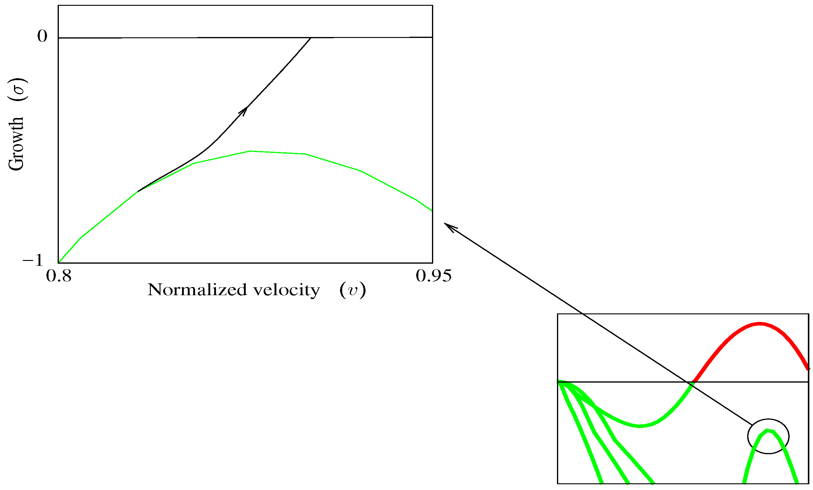
Figure 10.
Optimal path: σ-ω, black curve with arrow indicating tracking direction (Green means stable).
Figure 10.
Optimal path: σ-ω, black curve with arrow indicating tracking direction (Green means stable).

Figure 11.
LCO from the optimal path (black curve with arrow indicating tracking direction) (Green means stable, red means unstable).
Figure 11.
LCO from the optimal path (black curve with arrow indicating tracking direction) (Green means stable, red means unstable).

Figure 12.
Complete LCO boundaries, v-η and v-ω views (Green means stable, red means unstable).
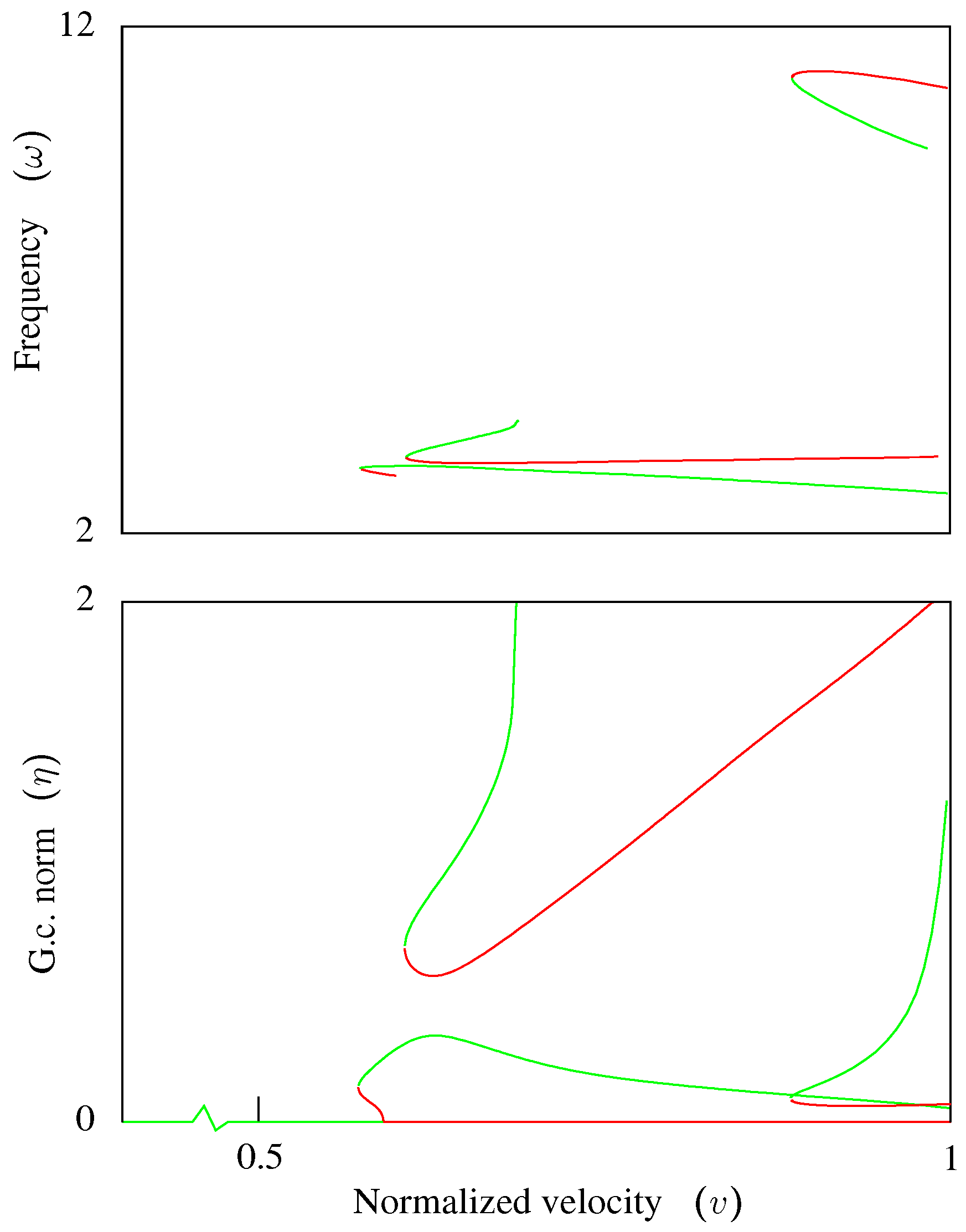
Figure 13.
Reduction of an LCO amplitude with control system parameters (Green means stable, red means unstable).
Figure 13.
Reduction of an LCO amplitude with control system parameters (Green means stable, red means unstable).

Figure 14.
Bifurcation in a V-σ-ω process. Arrows indicate the direction of positive μ, the blue curve arises from the bifurcation (Green means stable, red means unstable).
Figure 14.
Bifurcation in a V-σ-ω process. Arrows indicate the direction of positive μ, the blue curve arises from the bifurcation (Green means stable, red means unstable).
© 2016 by the author; licensee MDPI, Basel, Switzerland. This article is an open access article distributed under the terms and conditions of the Creative Commons Attribution (CC-BY) license (http://creativecommons.org/licenses/by/4.0/).
Share and Cite
MDPI and ACS Style
Meyer, E.E. Continuation Methods for Nonlinear Flutter. Aerospace 2016, 3, 44. https://doi.org/10.3390/aerospace3040044
AMA Style
Meyer EE. Continuation Methods for Nonlinear Flutter. Aerospace. 2016; 3(4):44. https://doi.org/10.3390/aerospace3040044
Chicago/Turabian StyleMeyer, Edward E. 2016. "Continuation Methods for Nonlinear Flutter" Aerospace 3, no. 4: 44. https://doi.org/10.3390/aerospace3040044
Note that from the first issue of 2016, this journal uses article numbers instead of page numbers. See further details here.