Chirp Signals and Noisy Waveforms for Solid-State Surveillance Radars

Abstract

Since the advent of “pulse compression” radar, the “chirp” signal (Linear Frequency Modulation, LFM) has been one of the most widely used radar waveforms. It is well known that, by changing its modulation into a Non-Linear Frequency Modulation (NLFM), better performance in terms of Peak-to-Sidelobes Ratio (PSLR) can be achieved to mitigate the masking effect of nearby targets and to increase the useful dynamic range. Adding an appropriate amplitude modulation, as occurs in Hybrid-NLFM (HNLFM), the PSLR can reach very low values (e.g., PSLR < −60 dB), comparable to the two-way antenna sidelobes in azimuth. On the other hand, modern solid-state power amplifier technology, using low-power modules, requires them to be combined at the Radio Frequency (RF) stage in order to achieve the desired transmitted power. Noise Radar Technology (NRT) represents a valid alternative to deterministic waveforms. It makes use of pseudo-random waveforms—realizations of a noise process. The higher its time-bandwidth (or BT) product, the higher the (statistical) PSLR. With practical BT values, the achievable PSLR using pure random noise is generally not sufficient. Therefore, the generated pseudorandom waveforms can be “tailored” (TPW: Tailored Pseudorandom Waveforms) at will through suitable algorithms in order to achieve the desired sidelobe level, even only in a limited range interval, as shown in this work. Moreover, the needed high BT, i.e., the higher time duration T having fixed the bandwidth B, matches well with the low power solid-state amplifiers of Noise Radar. Focusing the interest on (civil) surveillance radar applications, such as ATC (Air Traffic Control) and marine radar, this paper proposes a general review of the two classes of waveforms, i.e., HNLFM and TPW.

1. Introduction

For any new radar, the waveforms design is a key element, in which conflicting requirements have to be satisfied, i.e., (to mention the main ones), range resolution and accuracy (defined as the degree of conformance between the estimated or measured position and the true position), dynamic range, Multiple-Input Multiple-Output (MIMO) or polarimetric channels orthogonality, Low Probability of Intercept (LPI) [1,2,3], low interference to other apparatuses [4], and best exploitation of the transmitter power with a low (or unitary) crest factor. To mitigate the masking effect of nearby targets [5], the sidelobe level of the autocorrelation function of the transmitted pulse has to reach very low values comparable to the two-way antenna sidelobes in azimuth (typical of marine radars). Waveform design is of paramount interest in weather radar community, as solid-state and phased-array technology is being increasingly used also there. However, in that community the Integrated Sidelobe Level (ISL) is of interest. In this paper, mostly related to man-made targets (planes, ships) the peak sidelobe level is considered. This approach leads to specify the Peak-to-Sidelobes Ratio (PSLR) typically better than −60 dB [6,7]. One way to meet this requirement is the use of sidelobe-suppression filters in reception. However, these sidelobe-suppression filters [8,9] add Signal-to-Noise-Ratio (SNR) losses and an increase of the Doppler mismatch effect.

Alternatively, the optimal design of “chirp” radar waveforms [10,11,12], may be considered. Since the advent of “pulse compression” radar, the “chirp” signal (Linear Frequency Modulation, LFM) has been one of the most widely used radar waveforms. It is well known that, by changing its modulation into a Non-Linear Frequency Modulation (NLFM) [13,14,15], better performance in terms of PSLR can be achieved.

Historically, the design of chirp radar in the Western was made public in the 1960s [16] and, in the Eastern world, in the works (1950s) by Yakov Shirman [17], who received the IEEE Pioneer Award in 2009 “For the independent discovery of matched filtering, adaptive filtering, and high-resolution pulse compression for an entire generation of Russian and Ukrainian radars” [18,19].

The “chirp” theory is well established and is related to the Stationary Phase principle [10,12,20]: for a large enough number of independent samples, or product (also called Compression Ratio, or BT) between time duration T and bandwidth B, the group delay of a LFM signal is proportional to the instantaneous frequency. Moreover, the spectrum of the LFM signal after the matched filtering is quasi-rectangular, with constant amplitude and linear phase in the bandwidth B (and ideally, zero amplitude outside it). Its autocorrelation has a time duration 1/B and an unacceptable PSLR about 13.2 dB below the main peak. The sidelobes can be lowered by using an NLFM law, which can be easily designed by means of the well-known spectral windows [13,20]. However, this method, which relies on the Stationary Phase method, works well when BT is “large” (in practice for BT greater than a few thousands) but becomes less and less effective when BT decreases, as occurs in various civil applications like ATC (Air Traffic Control) radar and marine (or navigation) radar.

A new design method to cope with the sidelobe problem has been presented in [21,22], leading to a kind of Hybrid NLFM (HNLFM) whose amplitude, however, is not constant during the duration T of the signal. Such a requirement creates implementation problems with the widely-used saturated (C-class) power amplifiers. This family of waveforms is enhanced and analyzed in the following.

The power solid-state technology is increasingly used for radar transmitters using microwave transistor amplifiers leading, in most cases, to production/generation power issues. In fact, to achieve the typical medium-range for air or sea surveillance of civil targets, i.e., about 90 to 110 km (50 to 60 NM, Nautical Mile), a peak power of a few tens of kW has to be transmitted with a duty cycle around 10%. This power requirement is met by combining about 16 solid-state power modules at the Radio Frequency stage, typically emitting 50 to 100 W each. The pertaining implementation is not easy [23], since it should introduce low losses to minimize the attenuation of the coming through signal. It should also present good isolation between input/output ports so that each module is not influenced by the other, and finally, it should provide a well-matched circuitry to maximize the power transfer without occurring in load pulling. Apparatus size and weight can also increase if a large number of solid-state modules are needed. The high power requirement becomes more problematic if the before mentioned HNLFM signal is used because of its very precise amplitude modulation.

Another method, technically unrelated to the HNLFM, is the Noise Radar Technology (NRT). It represents a valid candidate to overcome the high-power stage issue. It makes use of pseudo-random waveforms, realizations of a Gaussian noise process [24]. The higher their time-bandwidth (or BT) product, the higher their (statistical) PSLR. In fact, since the PSLR is related to how much the waveform is equal to itself, the number of independent samples (with their phases) represents the degree of freedom available to make the correlation sidelobes as low as possible. Using pure random noise, practical BT values are generally not large enough to achieve PSLR. Therefore, the generated pseudorandom waveforms should be “tailored” (TPW: Tailored Pseudorandom Waveforms) at will through suitable algorithms [25] in order to achieve the desired sidelobe level. The suppression can also be applied over a limited range interval, as will be shown throughout this paper. Since the PSLR increases with the signal time duration T (assuming a fixed bandwidth B), we consider a 100% duty cycle operation for NRT with separated transmitting and receiving antennas. Then the architecture considered is a bistatic radar with co-located antennas, with low electromagnetic coupling between them. This architecture allows us to lengthen up the signal to the Waveform Repetition Time (WRT) which is the equivalent of the Pulse Repetition Time (PRT) for pulsed radar. This framework provides some advantages of the TPW approach over the pulsed HNLFM, including:

• the longer time duration allows to lower the transmitted peak power (with respect to an equivalent pulse compression radar) by about a figure of approximately 30 times, keeping unchanged the overall system requirements (e.g., maximum range, range resolution, bandwidth allocation) for the same application;
• the lower transmitted power calls for less solid-state modules to be combined, easing the radar transmitter architecture;
• a large number of quasi-orthogonal waveforms can be transmitted, alleviating mutual interference problems and paving the way for an MIMO operation [26,27].

The drawbacks of TPW include the dual antenna configuration (typical of Continuous Wave (CW) radars) as well as the burden of the real-time computation of the cross-ambiguity function. However, the matched filter approach can be successfully used. Design criteria and ensuing comparison of deterministic and pseudo-random waveforms are shown hereafter.

This paper focuses the attention on two waveform classes: HNLFM and TPW, suitable to be used in (civil) surveillance radar applications, such as ATC and marine radar. Most of this paper is a review of (many) works, some unpublished, by the authors.

The paper is organized as follows: Section 2 describes the deterministic waveforms design and compares classical pulse compression waveforms with the novel ones; Section 3 shows a different approach to pulse compression based on random waveforms (noisy signals) making use of CW operation; finally, Section 4 reports conclusions and future perspectives.

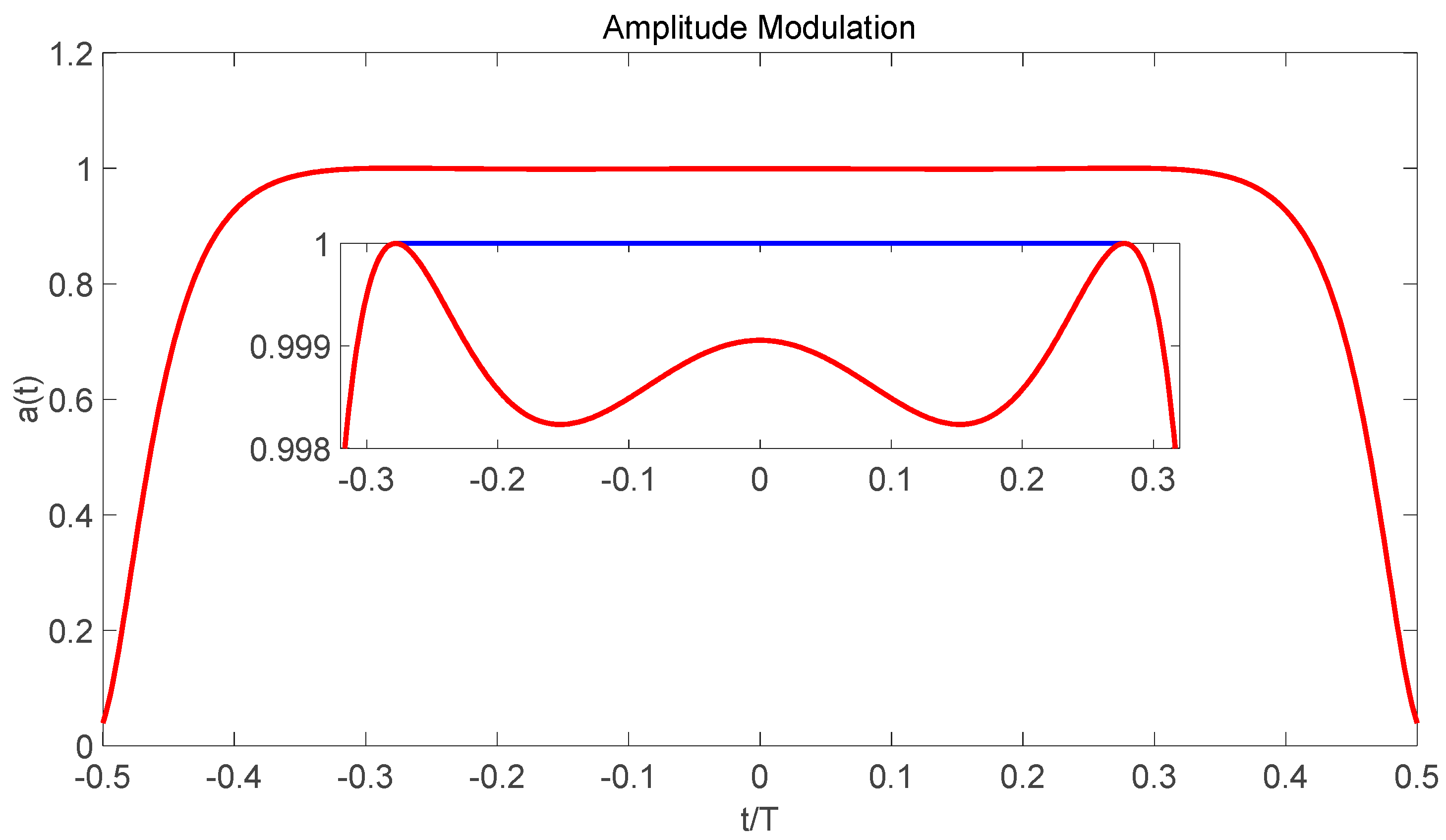
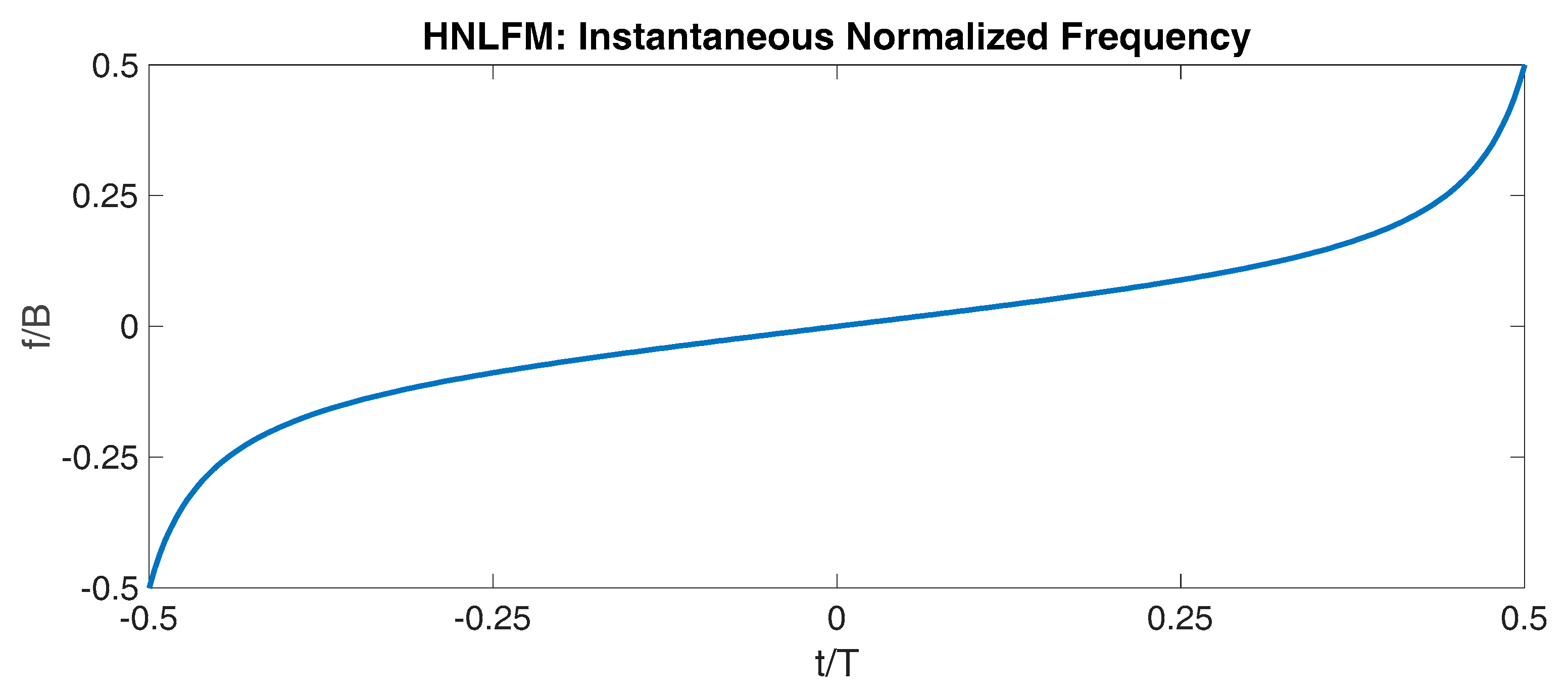
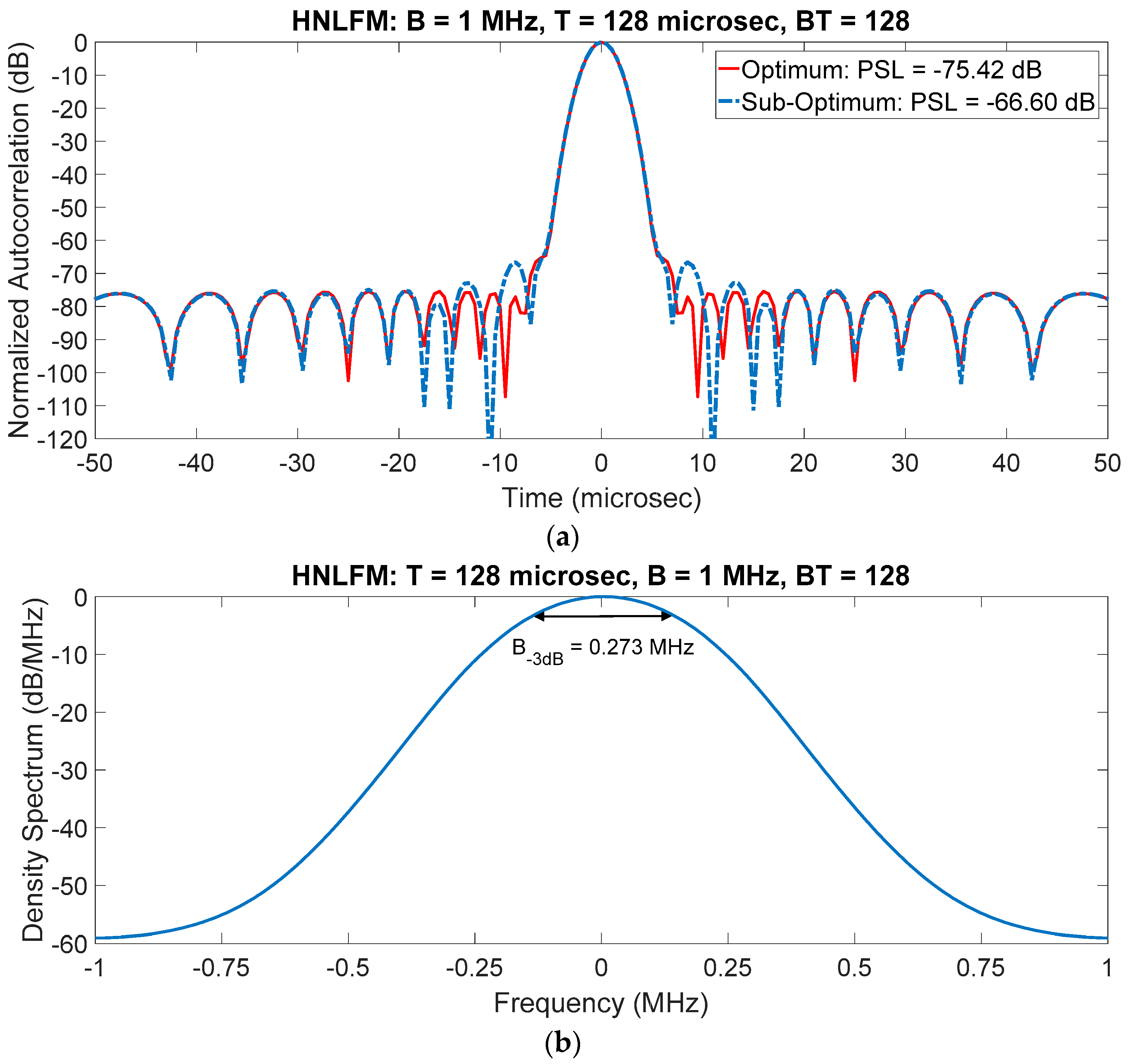
2. Deterministic Waveforms Design

The complex envelope of a generic signal, modulated both in Amplitude and in Phase (AM-PM), is:

$$s\left(t\right)=a\left(t\right)e^{j\mathsf{\varphi }\left(t\right)} ,$$

(1)

where $a\left(t\right)$ and $\mathsf{\varphi }\left(t\right)$ denote respectively the AM and PM modulation. The stationary phase principle [10,16] establishes that, at the instantaneous frequency ${\mathsf{\omega }}_t$ the amplitude spectrum ${\left|S\left({\mathsf{\omega }}_t\right)\right|}^2$ of a given signal $s\left(t\right)$, having the amplitude $a\left(t\right)$, can be approximated as [10]:

$${\left|\mathrm{S}\left({\mathsf{\omega }}_t\right)\right|}^2\cong 2\mathsf{\pi }\frac{a^2\left(t\right)}{\left|{\mathsf{\varphi }}^{″}\left(t\right)\right|} ,$$

(2)

i.e., the energy spectral density at the frequency ${\mathsf{\omega }}_t={\mathsf{\varphi }}^{\prime }\left(t\right)$ (in radians) is larger when the rate of change of ${\mathsf{\omega }}_{\mathrm{t}}$ is smaller. From Equation (2) the amplitude modulation function $a\left(t\right)$ can be evaluated as:

$$a\left(t\right)\cong \sqrt{\frac{1}{2\mathsf{\pi }}{\left|S\left({\mathsf{\varphi }}^{\prime }\left(t\right)\right)\right|}^2\left|{\mathsf{\varphi }}^{″}\left(t\right)\right|} .$$

(3)

However, the validity of the stationary phase approximation depends on the compression ratio BT, and it should be considered reliable only for large BT (in practice, greater than a few thousands). It is less and less effective when a low BT is required, as it happens in various radar applications. Considering the Millett waveform, i.e., a “cosine squared on a pedestal” weighting [13], the output of the Matched Filter (MF) reaches the theoretical PSLR of −42 dB only when BT is greater than about one thousand. For any lower compression ratio, a convenient frequency modulation function (in radians) can be obtained as a weighted sum of the Non-Linear tangent FM term and the LFM one, hence the name Hybrid-NLFM [21,22]:

$${\mathsf{\varphi }}^{\prime }\left(t\right)=\mathsf{\pi }B\left\{\alpha \frac{1}{tg\left(\mathsf{\gamma }\right)}tg\left(\frac{2\mathsf{\gamma }t}{T}\right)+\left(1-\alpha \right)\frac{2t}{T}\right\} ,$$

(4)

where $\alpha \in \left(0, 1\right)$ is the relative weight between the linear and the tangential terms, B is the swept frequency (nearly equal to the signal’s bandwidth), $\mathsf{\gamma }$ is the Non-Linear tangent FM rate and, being $t\in \left[-\frac{T}{2},+\frac{T}{2}\right]$, T denotes the pulse-width.

If $s\left(t\right)$ is a signal with a Gaussian spectrum: ${\left|S\left({\mathsf{\omega }}_t\right)\right|}^2=\exp \left(-\mathsf{\beta }\frac{{\mathsf{\omega }}_t^2}{B^2}\right)$ with $\mathsf{\beta }=1$, using the optimized values of $\mathsf{\alpha }$ and $\mathsf{\gamma }$ as evaluated in [21,22] (i.e., those values that reach the optimum PSLR maximizing the transmission efficiency: $\eta =\frac{1}{T}{\int }_{-T/2}^{+T/2}{a}^2\left(t\right)dt$), the energy loss results as low as 0.58 dB with respect to the case of unity amplitude. Inserting Equation (4) into Equation (3), the amplitude modulation has been evaluated as shown in Figure 1. Zooming around $a\left(t\right)=1$, i.e., in the interval (−0.3, 0.3), some ripples of the relative amplitude order of ${10}^{-3}$ are observed. In Figure 2, the corresponding instantaneous frequency modulation is shown.

Figure 3 shows the PSLR of the matched filter output for the optimized waveform (solid line-circles). With BT decreasing, the approximation due to the principle of the stationary phase becomes worse and worse causing an increase in the PSLR. However, with BT = 64 the PSLR (−51 dB) is still compatible with many applications, and for BT = 128 the PSLR is −75 dB, which is suited to most applications.

These excellent theoretical results (circles in Figure 3) are only possible if the amplitude weighting is the one shown in Figure 1 (red line) with the instantaneous frequency of Figure 2.

In practice, it may be hard to implement the requirement on $a\left(t\right)$, with ripples of the order of 1 over 1000. In general, if a PSLR level of −60 dB is required, a simple rule of thumb tells us that the fidelity of the waveform, in terms of (I, Q) or (Amplitude, Phase) shall be better than 1:1000, or 10 bits, no matter how the waveform is designed. It is widely known—from many practical experiences (unfortunately, not available in the open literature)—that hardware imperfections increase the PSLR with respect to the “ideal” compressed waveform. This means that if the required PSLR is for example −60 dB, the intrinsic level of the waveform (which is our focus) has to be −67 dB, the difference between these figures depending, of course, on the stability/linearity of the hardware. In a recent private communication [28] it is explained that: “In one case, related to a NAVICO civil marine radar using GaN for the solid state amplifier, and a non-linear FM, amplitude-weighted pulse with BT = 150, the measured PSLR is −55 dB, versus the “ideal” −60 dB of the waveform”. So, the effect of hardware is significant but not dramatic, and can be controlled with a careful design.

If the amplitude of the transmitted signal is kept constant (the power amplifier working in saturation) with the instantaneous frequency of Figure 2, the theoretical PSLR increases by about 25–30 dB. An improvement can be obtained using a sub-optimum waveform where the ripples shown in the zoom of Figure 1 are removed imposing $a\left(t\right)=1$ in this interval (dashed line in Figure 1). The PSLR of this “sub-optimum” waveform results only 10–20 dB worse than the optimized signal when $BT\ge 128$ (diamonds-line in Figure 3). Figure 4 shows the half-power pulse width (${\mathsf{\tau }}_{3\mathrm{dB}}$) versus the compression ratio BT. The values are compared with the ones of the LFM, i.e., ${\mathsf{\tau }}_{3\mathrm{dB}}=\frac{1}{B}$.

For $BT=128$ (frequency swept of $B=1 \mathrm{MHz}$ and duration $T=128 \mathsf{\mu }\mathrm{s}$), Figure 5a shows the compressed pulse, while Figure 5b reports its spectrum. The PSLR reaches about −75 dB for the optimum waveform case and −66 dB for the sub-optimum one, still compatible for most applications, e.g., lower than the typical two-way antenna sidelobes in azimuth. The range resolution, i.e., $\mathrm{\Delta }R=\frac{c}{2B_{-3\mathrm{dB}}}$ ($B_{-3\mathrm{dB}}$ representing the −3 dB bandwidth), is about 550 m. It is worth clarifying that the bandwidth of a waveform is very important when spectral limitations apply, which is the case of most civil radar. Of course, bandwidth values only give a rough indication of the range resolution, whose correct numerical value is of course the −3 dB width of the output of the reception filter, either matched or possibly mismatched for some reason.

To improve the resolution, maintaining the same pulse duration, the swept frequency has to be increased, with the only practical limitation being the restricted use of the spectrum.

3. Noise Radar Technology

The HNLFM capability to get very low sidelobes of the compressed pulse is strictly dependent on the ability of the signal generation and amplification chain, including the RF power amplifier, to faithfully reproduce the amplitude modulation of Figure 1, calling for highly linear A-class amplifiers. Moreover, the available bandwidth is not fully exploited because of the particular frequency law of Equation (4), which is the main law responsible for the low sidelobe level.

Noise Radar Technology (NRT) [29,30,31,32,33,34,35] may be a valid alternative to overcome the high-power amplitude modulation issue. NRT makes use of pseudo-random waveforms that are realizations of a Gaussian band-limited random process [24]. These “pure noise” realizations, once generated and stored, are not strictly random anymore as they act as deterministic signals with known PSLR, range resolution and ambiguity function. The number of different possible realizations to be used is theoretically unlimited (modern pseudorandom numbers generator can reach a period of 2¹⁴⁹² [36], as implemented in Matlab generator—practically infinity), so that each radar can operate with its own radar signal, possibly different from the others. Being noisy, the waveforms themselves possess a low enough degree of mutual cross-correlation to pave the way for distributed MIMO operation with a low level of mutual interferences [27] even operating at the same, or nearby, carrier frequency.

For a pure noise waveform, the PLSR value does not strongly depend on the amplitude modulation [24] but, rather, on the Time Bandwidth product BT. The bandwidth being limited by the application context (e.g., about 50 MHz, and 200 MHz as a maximum, for marine radar), BT may be increased at will by selecting a continuous wave (CW) architecture instead of the pulsed one, keeping unchanged the compression processing (computation of the correlation or the ambiguity function) at the receiver side. The power can be significantly lowered with respect to an equal-performance pulse radar architecture.

3.1. Power Budget

Let us consider a typical maximum range of 150 km (80 NM) with a range resolution of 150 m. A comparison between pulsed HNLFM and CW noise radar can be done while keeping the transmitted energy constant. For this purpose, let us consider the saturated HNLFM since the power loss with respect to the optimal amplitude modulation is only 0.58 dB. In a CW architecture, the maximum delay due to range is generally set as one-fourth of the Waveform Repetition Time (WRT), which corresponds to the signal time duration if we neglect the data processing time between consecutive sweeps:

$$\frac{WRT}{4}=\frac{2·R_{\max }}{c} .$$

(5)

For a maximum range of 150 km, it is required that: $\frac{WRT}{4}=\frac{2·150000 \left(\mathrm{m}\right)}{3·{10}^8 \left(\mathrm{m}/\mathrm{s}\right)}=1 \mathrm{ms}$, i.e., $WRT=4000 \mathsf{\mu }\mathrm{s}$, i.e., $4096 \mathsf{\mu }\mathrm{s}$ in order to work with power-of-two values. Knowing the time duration of the noise signal ($WR{T}_{noise}$) together with the HNLFM pulse width ($T_{HNLFM}$), the relationship between the needed peak powers can be evaluated as:

$$P_{noise}=P_{HNLFM}·\frac{T_{HNLFM}}{WR{T}_{noise}} ,$$

(6)

where $P_{noise}$ and $P_{HNLFM}$ are respectively the peak power of CW noise and pulsed radar. With $WR{T}_{noise}=4096\mathsf{\mu }\mathrm{s}$ and $T_{HNLFM}=128\mathsf{\mu }\mathrm{s}$, it results: $P_{noise}=0.03125·P_{HNLFM}$. The equality holds also for the optimal amplitude modulated HNLFM if the 0.58 dB power loss is considered. Equation (6) states that the required power for a CW noise radar is about 15 dB lower than the peak power required for a pulsed radar, keeping unchanged the maximum range. Lowering the transmitted power means less solid-state modules and a straightforward RF power production/generation design.

The generation of M independent pure noise band-limited signals is shown in Figure 6. The ($I,Q$) samples are generated through a white Gaussian random process. The signal to be filtered by the frequency window $H\left(f\right)$ is ${\left\{x_i\right\}}_{i=1}^N$ where $N$ is the number of generated samples and $x_i$ the $i\mathrm{th}$ complex $\left(I,Q\right)$ sample.

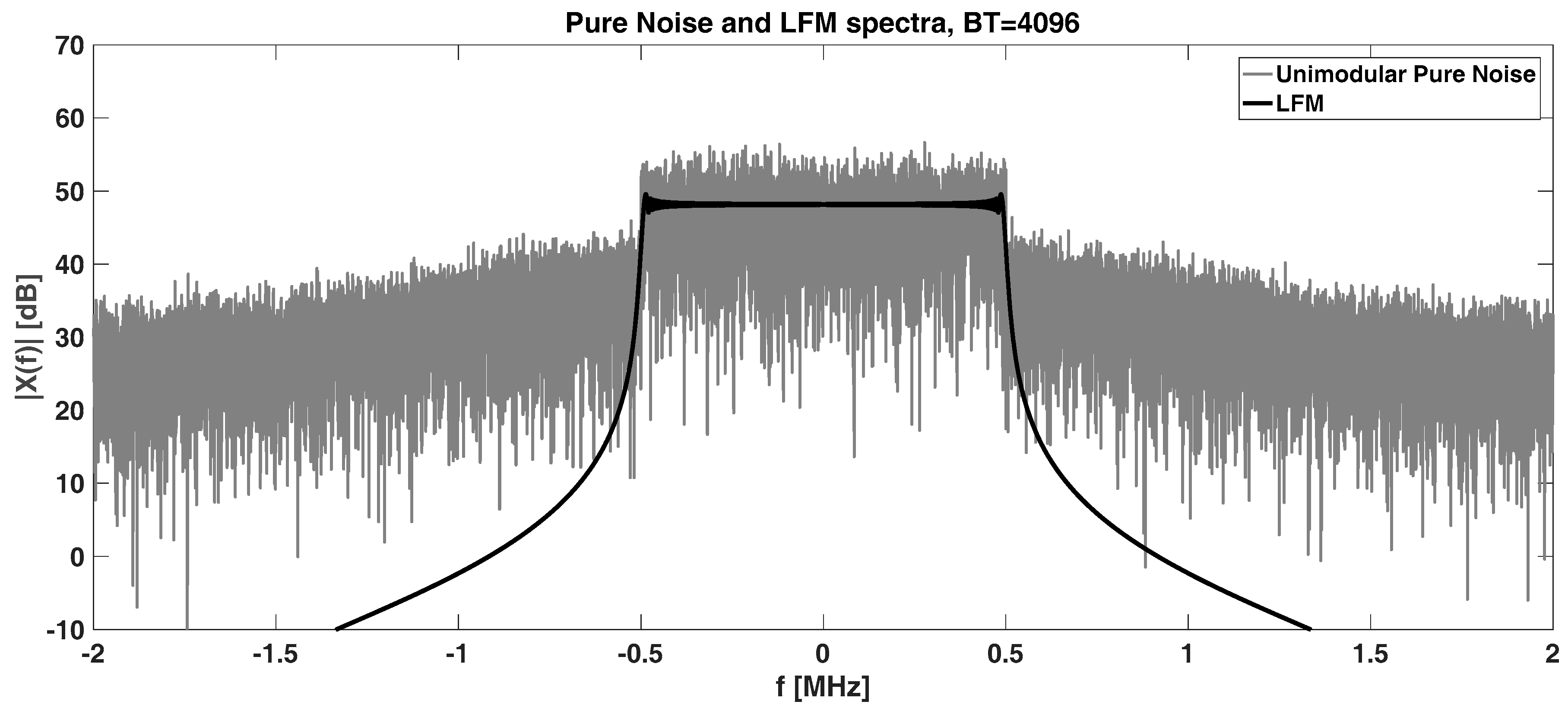
3.2. Unimodular Pure Noise

Being a white process, the signal has to be band-limited with a proper frequency window $H\left(f\right)$ which can be any, e.g., Blackman–Nuttall [37] or simply rectangular. In this paper, we consider the rectangular frequency window to fully exploit the available bandwidth; other windows can be used to gain a slight improvement in PSLR value. After the frequency domain windowing, the signal amplitude is saturated to the maximum (i.e., a unimodular signal is obtained) value through a Zero-Memory-Non-Linear (ZMNL) transformation, while the phase is kept unchanged. Since the $\left(I,Q\right)$ samples come from a random process, at each run, the algorithm provides different realizations having the same average performances in terms of PSLR and cross-correlation level, while the range resolution only depends on the used $H\left(f\right)$. Figure 7 shows the spectrum of the unimodular band-limited pure noise and the spectrum of a LFM signal having the same BT. The 1 MHz bandwidth is fully exploited.

Once compressed by the matched filter, the pure noise and the LFM give a range resolution of $\mathrm{\Delta }R=150\mathrm{m}$ ($1 \mathsf{\mu }\mathrm{s}$) as shown in Figure 8. In the first 5–10 $\mathsf{\mu }\mathrm{s}$, the secondary lobes of pure noise are slightly fluctuating (the PSLR is comparable to the LFM). For far lobes, the PSLR is empirically related to the BT [24] by Equation (7):

$$PSLR=-10\cdot lo{g}_{10}\left(BT\right)+k\left[\mathrm{dB}\right] ,$$

(7)

with $k$ of the order of 10–13 dB, which corresponds, for BT = 4096, to −23 dB (see Figure 8). The cross-correlation level between two independently generated pure noise signals is of the same level as the autocorrelation sidelobes, excluding the central zone. The advantage of the pure noise signal with respect to the HNLFM signal is two-fold: a narrower bandwidth to get the required range resolution and a cross-correlation level at the same value as its autocorrelation sidelobes.

The main reason suggesting the use of noisy signals, beyond the MIMO application, is their capability to be tailored at will to reach better PSLR values, e.g., −60 dB as discussed above.

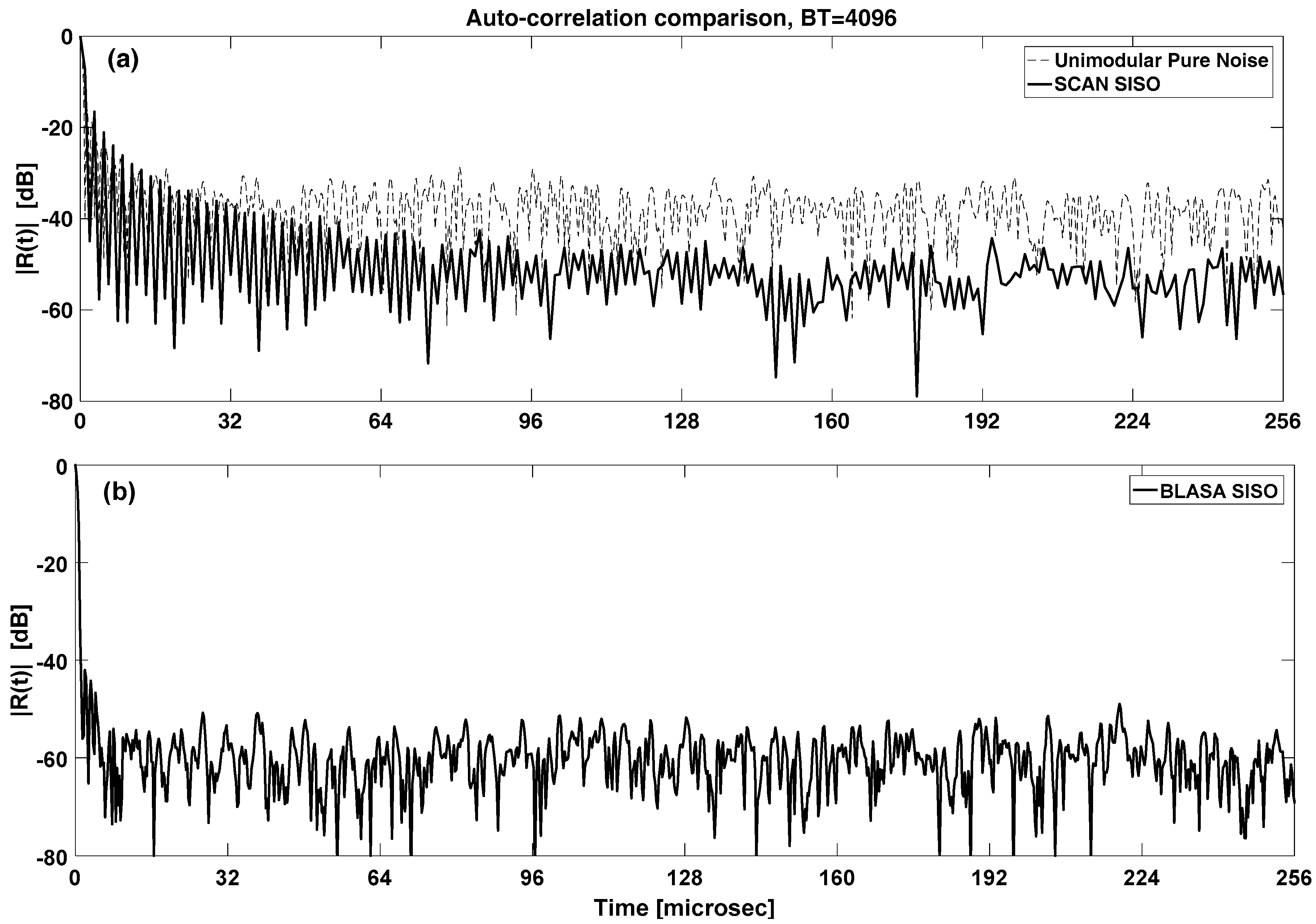
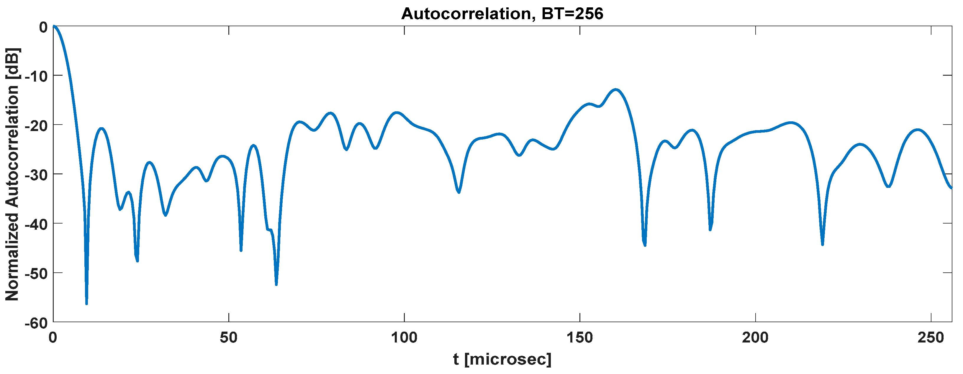
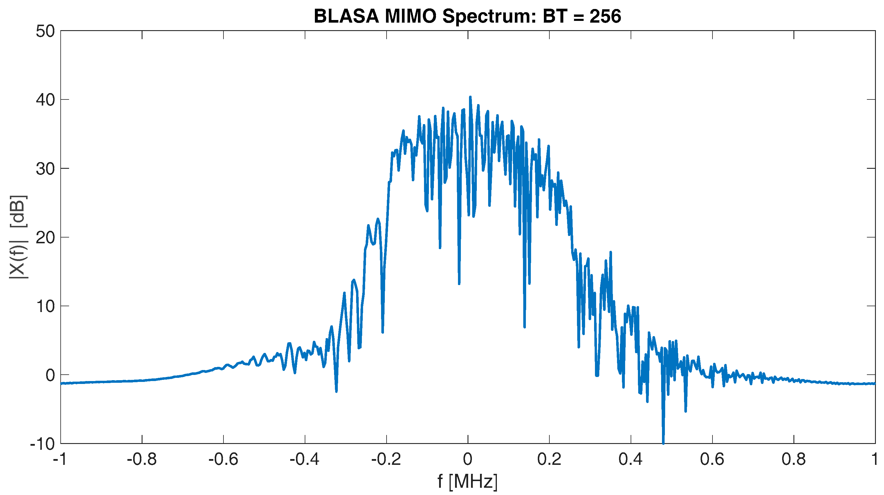
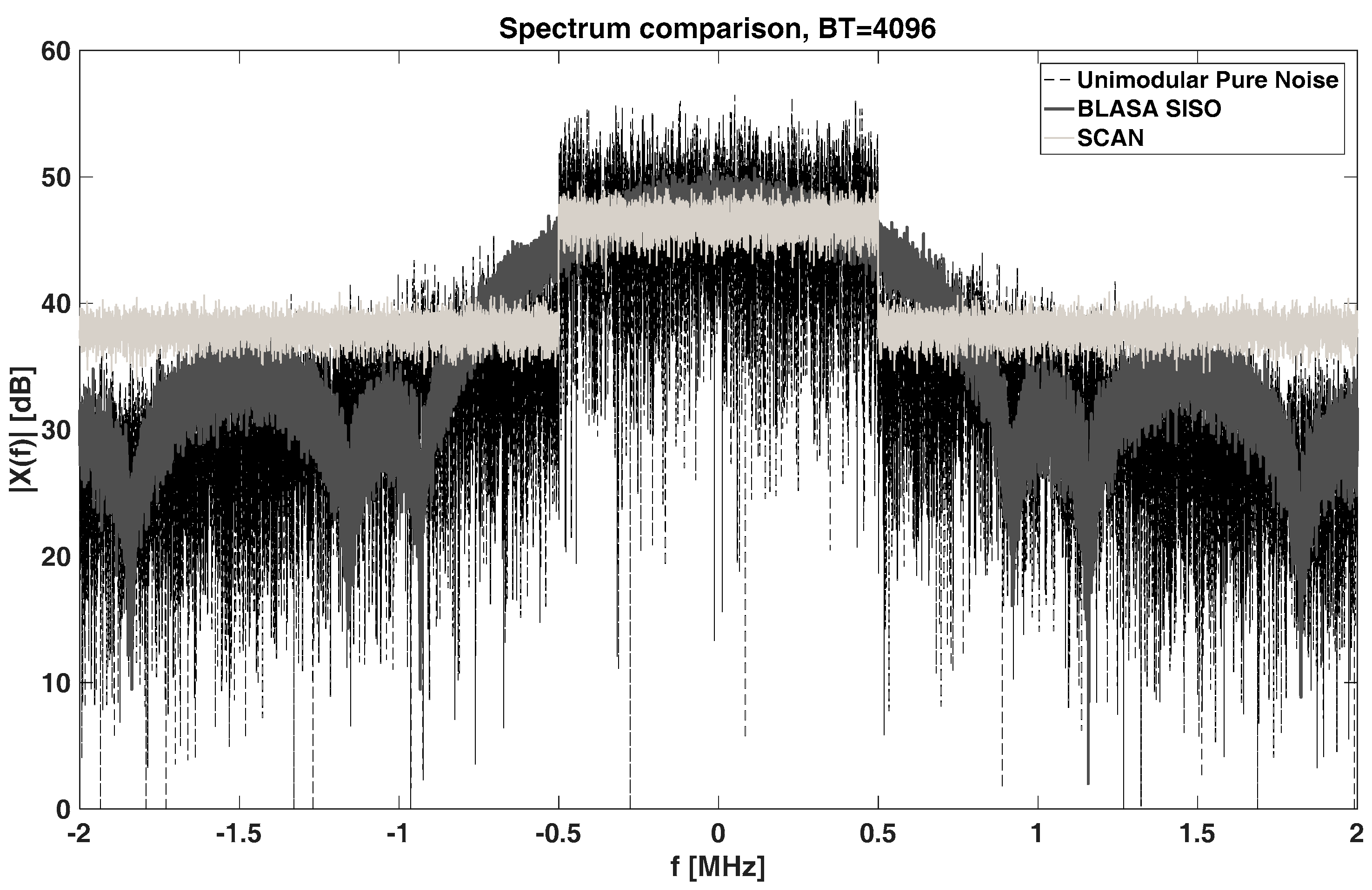
3.3. Range Sidelobe Suppression Algorithms

Many approaches have been used in the past years to cope with the range sidelobe problem, starting from the time (or frequency) weighting of the received signal [10,11], to the modern algorithms able to generate signals with suitable autocorrelation characteristics without the need of sidelobe suppression in reception. The main difference between these two approaches is that, using the generation algorithms, significant complexity is demanded to the generation side in terms of computational burden to achieve a “useful” waveform. In any case, this issue can be trivially overcome by offline generating a large enough set of noisy waveforms ready to be transmitted, and stored in a mass memory [31].

Generally, a noise generation algorithm starts from a random process realization (e.g., the unimodular, band-limited one, see Figure 6) and runs in order to minimize a certain objective function with defined constraints. In this case, the objective function is the PSLR and the constraints are the limited bandwidth and the unity amplitude needed to fully exploit the solid-state amplifier. Often, due to convergence considerations, the Integrated-Side-Lobe (ISL) is minimized instead of the PSLR because the former is an integrated value over all the sidelobe region while the latter is only a local value that can rapidly change point by point.

A well-known sidelobe suppression algorithm family is the Cyclic Algorithm New (CAN) [25] that provides several interesting ways to approach the suppression problem. To suit the algorithm to particular needs, the authors of this paper have developed a new algorithm to generate noisy waveforms having a limited bandwidth and an unimodular amplitude, with the possibility to tune the suppressed zone length depending on the particular application. In the following, some results are shown and discussed, highlighting advantages and drawbacks.

In some applications, the matched filter output is performed by a periodic correlation between the radar return and the reference, which can significantly differ from the aperiodic case. The periodic approach can be considered in the case of FFT implementation, with it being a spectrum product, i.e., a circular correlation. In this paper, only the aperiodic correlation is discussed.

CAN algorithms [25] have been developed both for aperiodic and periodic cases; in general, there are no large basic differences between them. The main idea is to minimize the difference between the obtained and the desired autocorrelation functions through a process that runs cyclically until a stop criterion is satisfied, e.g., the difference between two consecutive steps is less than a given threshold. The constraints to be satisfied within this minimization lead to different algorithms belonging to the CAN family. These constraints can be the unit amplitude, the number of suppressed sidelobes as well as the mainlobe width (i.e., the needed bandwidth) or others.

Especially in MIMO radar configuration, a number of M orthogonal waveforms are required to discriminate, after the matched filter, the m^th signal among the others. For this purpose, the CAN family also provides a “MIMO” version for the algorithms in which the quantity to be minimized is the difference between the obtained and the desired covariance matrix [25], until a stop criterion is reached.

The main drawback of the CAN algorithms is their inability to manage the bandwidth increase, i.e., the mainlobe of the signal generated by using the CAN algorithm is very narrow. In fact, these algorithms prefer a deep sidelobe suppression at the expense of having a full-Nyquist occupied bandwidth, which unfortunately is not suitable for applications in which spectrum regulations must be met. Only one CAN algorithm (Stopband CAN (SCAN) [25]) is able to manage the spectrum constraint. In this study, the SCAN has been applied to generate noise unimodular signals with BT = 4096 and B = 1 MHz. The related aperiodic autocorrelation is shown in Figure 9a. Keeping BT unchanged, the SCAN algorithm improves the PSLR by about 20 dB with respect to the unimodular noise from which the algorithm starts. The mainlobe is kept wide since the SCAN spectrum, shown in Figure 10, is well-shaped within the required 1 MHz bandwidth.

The drawback of the SCAN algorithm is that the sidelobes close to the mainlobe are still quite high. To overcome the issue, the authors have developed the BLASA (Band Limited Algorithm for Sidelobes Attenuation) algorithm whose result is shown in Figure 9b. It comes from the same CAN idea and provides very low sidelobes even in the area close to the mainlobe. It is called “SISO” (Single Input, Single Output) because a single waveform is generated at each run. The BLASA SISO spectrum is shown in Figure 10 and it is still well shaped within the allowed 1 MHz bandwidth, providing a range resolution of 150 m.

Being a “SISO” algorithm, BLASA does not lower the cross-correlation level between two independently generated waveforms. Hence, their cross-correlation is at the same level as the initial unimodular pure noise.

As in the CAN family, even for the BLASA SISO, a “MIMO” version exists which is able to jointly generate a number M of waveforms at each run, i.e., M signals belonging to the same set. The BLASA MIMO has been developed to manage the suppression of both auto and cross-correlation functions, still keeping the bandwidth limited.

Due to the limited number of samples that BLASA MIMO can manipulate, the joint suppression region in cross and auto correlations cannot be as long as the whole length of the pulse. The length of the suppressed zone depends on the number M of the waveforms in the generated set: the lower M, the longer the suppressed length. Moreover, the suppressed zone length depends on the amplitude constraint: it increases if amplitude modulation is allowed while it decreases if the unimodular constraint is applied. Hereafter, only the unimodular case will be considered.

Figure 11 shows the BLASA MIMO compressed pulse with M = 2 and the unimodular amplitude constraint. It is generated for BT = 256 which is the maximum value at which the current algorithm version can work. The occupied bandwidth is always B = 1 MHz but, as it happens with the HNLFM, the −3 dB bandwidth is a quarter of the total occupied bandwidth.

The limited length of the suppressed zone represents a valid tool to mitigate the clutter effect, especially in the proximity of the mainlobe, i.e., the target’s closest range cells. Because of the narrow −3 dB bandwidth (see Figure 12), the mainlobe is four times wider than the expected 150 m, which corresponds to a 1 MHz bandwidth.

Nevertheless, this behaviour is deterministic and can be overcome by properly choosing the signals’ occupied bandwidth. The big advantage of the BLASA MIMO pseudorandom signals with respect to the deterministic HNLFM is the possibility to coherently average the range sidelobes in azimuth. In fact, if the transmitted waveform changes each WRT within the dwell time, the averaged compressed pulse presents a sidelobe level reduced by the quantity [24]:

$$\mathrm{\Delta }SL=10\cdot {\log }_{10}\left(L\right) ,$$

(8)

where ΔSL is the lowering in the sidelobe level with respect to the not-averaged case and L is the number of coherently integrated returns.

Summing up all the considered waveforms,

Table 1. Comparison of algorithms (B_TOT denotes the swept frequency).

Algorithm	MIMO Version	Sidelobe Level and Suppression Interval	$\raisebox{1ex}{${\mathit{B}}_{\mathit{T}\mathit{O}\mathit{T}}$}\!\left/ \!\raisebox{-1ex}{${\mathit{B}}_{-\mathbf{3} \mathbf{d}\mathbf{B}}$}\right.$	Amplitude Modulation
HNLFM	No	−67 dB at BT = 4096	400%	Pseudo trapezoidal AM
Pure Unimodular Noise	No	−23 dB at BT = 4096	100%	Unimodular
SCAN	No	−45 dB at BT = 4096 (within 15%)	100%	Unimodular
BLASA SISO	No	−50 dB at BT = 4096	100%	Unimodular
BLASA MIMO	Yes	−30 dB at BT = 256 (within 12%) if unimodular amplitude with M = 2	400%	Unimodular

shows their comparison. Each algorithm is checked to verify whether it allows a MIMO version, the level of the sidelobes, the frequency occupancy and its capability to be coherently integrated.

The column “MIMO version” refers to the capability of jointly generated M waveforms with a cross-correlation level equal to the auto-correlation level. The frequency occupancy gives the information of how much the mainlobe is enlarged by the algorithm.

The SCAN sidelobe level refers to the zone within 15% of the whole length, as shown in Figure 9, while the −30 dB of BLASA MIMO is related to the suppressed area which is about 12% of the whole length when two signals (M = 2) are jointly generated with a unimodular amplitude.

4. Conclusions

The design of the transmitted signal is an increasingly important element in the development of modern radars. The availability of stable and accurate waveform generators and of real-time, high dynamic range digital correlators makes it possible to use, as radar signals, arbitrary waveforms with a number of degrees of freedom, i.e., independent samples, of the order of a thousand and even more, permitting pulse compression with a processing gain of the same order of magnitude. In this paper, two classes of novel waveforms for pulse-compression (and continuous-wave) radars have been discussed and evaluated: (i) a (deterministic) type of frequency modulated pulse with a “trapezoidal-like” amplitude modulation and; (ii) a subset of noisy waveforms in the Noise Radar Technology context. Both are designed in order to make the range sidelobes as low as possible, which are the main issue in the matched filter approach, both for pulsed and continuous-wave radars. A set of representative results has been shown in terms of sidelobe level, width of the main lobe and spectral occupancy. The selection of the particular waveform depends, of course, on the application.

References

1. Pace, P.E. Detecting and Classifying Low Probability of Intercept Radar; Artech House: Norwood, MA, USA, 2004. [Google Scholar]
2. Govoni, M.A. Low Probability of Interception of an Advanced Noise Radar Waveform with Linear-FM. IEEE Trans. AES 2013, 1351–1356. [Google Scholar] [CrossRef]
3. Galati, G.; Pavan, G.; De Palo, F. Noise Radar Technology: Pseudorandom Waveforms and their Information Rate. In Proceedings of the International Radar Symposium, Gdansk, Poland, 16–18 June 2014; pp. 123–128.
4. Harman, S. The Performance of a Novel Three-Pulse Radar Waveform for Marine Radar System. In Proceedings of the 5th European Radar Conference, Amsterdam, The Netherlands, 30–31 October 2008; pp. 160–163.
5. Blunt, S.D.; Gerlach, K. Adaptive Pulse Compression via MMSE estimation. IEEE Trans. AES 2006, 42, 572–584. [Google Scholar] [CrossRef]
6. De Witte, E.; Griffiths, H.D. Improved ultra-low range sidelobe pulse compression waveform design. Electron. Lett. 2004, 40, 1448–1450. [Google Scholar] [CrossRef]
7. Sarkar, T.K. An Ultra-low Sidelobe Pulse Compression Technique for High Performance Radar Systems. In Proceedings of the IEEE National Radar Conference, Syracuse, NY, USA, 13–15 May 1997; pp. 111–114.
8. Lohmeier, S.P. Adaptive FIR filtering of Range Sidelobes for Air and Spaceborne Rain Mapping. In Proceedings of the IEEE International Geoscience and Remote Sensing Symposium, Toronto, ON, Canada, 24–28 June 2002; Volume 3, pp. 1801–1803.
9. Ackroid, M.H.; Ghani, F. Optimum mismatched filters for sidelobe suppression. IEEE Trans. AES 1973, 9, 214–218. [Google Scholar] [CrossRef]
10. Cook, C.E.; Bernfeld, M. Radar Signals—An Introduction to Theory and Application; Artech House: Norwood, MA, USA, 1993. [Google Scholar]
11. Richards, M.A. Fundamentals of Radar Signal Processing; Section 4.6; McGraw Hill: New York, NY, USA, 2005. [Google Scholar]
12. Levanon, N.; Mozeson, E. Radar Signals; John Wiley & Sons: Hoboken, NJ, USA, 2004. [Google Scholar]
13. Millett, R.E. A Matched-Filter Pulse-Compression System Using a Nonlinear FM Waveform. IEEE Trans. AES 1970, AES-6, 73–77. [Google Scholar]
14. Doerry, A.W. Generating Nonlinear FM Chirp Waveforms for Radar; Sandia Report SAND2006-5856; Sandia National Laboratories: Albuquerque, NM, USA; Livermore, CA, USA, 2006. [Google Scholar]
15. Doerry, A.W. SAR Processing with Non-Linear FM Chirp Waveforms; Sandia Report SAND2006-7729; Sandia National Laboratories: Albuquerque, NM, USA; Livermore, CA, USA, 2006. [Google Scholar]
16. Klauder, J.R.; Price, A.C.; Darlington, S.; Albefsheim, W.J. The theory and design of chirp radars. Bell Syst. Tech. 1960, 39, 745–808. [Google Scholar] [CrossRef]
17. Yanovsky, F. Radar development in Ukraine. In Proceedings of the International Radar Symposium, Gdansk, Poland, 16–18 June 2014.
18. 2009 Pioneer Award. IEEE Trans. Aerosp. Electron. Syst. 2010, 46, 2139–2141.
19. Galati, G.; van Genderen, P. Special Section on Some Less-Well Known Contribution to the Development of Radar: From its Early Conception Until Just after the Second World War; URSI Radio Science Bulletin, No 358; URSI: Ghent, Belgium, September 2016; pp. 12–108. [Google Scholar]
20. Papoulis, A. Signal Analysis; McGraw Hill: New York, NY, USA, 1977. [Google Scholar]
21. Collins, T.; Atkins, P. Nonlinear frequency modulation chirps for active sonar. Proc. IEE Radar Sonar Navig. 1999, 146, 312–316. [Google Scholar] [CrossRef]
22. Zhiqiang, G.; Peikang, H.; Weining, L. Matched NLFM Pulse Compression Method with Ultra-low Sidelobes. In Proceedings of the 5th European Radar Conference, Amsterdam, The Netherlands, 30–31 October 2008; pp. 92–95.
23. Russell, M.; Marinilli, A.; Sullivan, F. Millimeter wave, solid-state amplifiers in radar and communication systems. In Proceedings of the IEEE MTT-S International Microwave Symposium Digest, San Francisco, CA, USA, 17–21 June 1996; pp. 53–56.
24. Galati, G.; Pavan, G.; De Palo, F. Generation of Pseudo-Random Sequences for Noise Radar Applications. In Proceedings of the International Radar Symposium, Gdansk, Poland, 16–18 June 2014; pp. 115–118.
25. He, H.; Li, J.; Stoica, P. Waveform Design for Active Sensing Systems—A Computational Approach; Cambridge University Press: Cambridge, UK, 2012. [Google Scholar]
26. Galati, G.; Pavan, G. Mutual interference problems related to the evolution of Marine Radars. In Proceedings of the 18th IEEE International Conference on Intelligent Transportation Systems, Las Palmas, Spain, 15–18 September 2015; pp. 1785–1790.
27. Galati, G.; Pavan, G.; De Palo, F. Compatibility problems related with pulse compression, solid-state marine radars. IET Radar Sonar Navig. 2016, 10, 791–797. [Google Scholar] [CrossRef]
28. Baroncelli, A.; NAVICO Rbu, Montespertoli, Florence, Italy. Personal communication, 1 February 2017.
29. Galati, G.; Pavan, G.; De Franco, A. Orthogonal Waveforms for Multistatic and Multifunction Radar. In Proceedings of the 9th European Radar Conference, Amsterdam, The Netherlands, 31 October–2 November 2012; pp. 310–313.
30. Stove, A.; Galati, G.; Pavan, G.; De Palo, F.; Lukin, K.; Kulpa, K.; Kulpa, J.S.; Maślikowski, Ł. The NATO SET-184 noise radar trials 2016. In Proceedings of the 17th International Radar Symposium, Krakow, Poland, 10–12 May 2016; pp. 1–6.
31. Galati, G. Coherent Radar. Patent PCT/IC2014/061454, 15 May 2014. [Google Scholar]
32. Galati, G.; Pavan, G.; De Palo, F.; Stove, A. Potential applications of noise radar technology and related waveform diversity. In Proceedings of the 17th International Radar Symposium, Krakow, Poland, 10–12 May 2016; pp. 1–5.
33. Stove, A.; Galati, G.; De Palo, F.; Wasserzier, C.; Erdogan, Y.A.; Kubilay, S.; Lukin, K. Design of a Noise Radar Demonstrator. In Proceedings of the 17th International Radar Symposium, Krakow, Poland, 10–12 May 2016; pp. 1–6.
34. Galati, G.; Pavan, G.; De Palo, F. On the potential of noise radar technology. In Proceedings of the Enhanced Surveillance of Aircraft and Vehicles (ESAV 2014), Rome, Italy, 15–16 September 2014; pp. 66–71.
35. De Palo, F.; Galati, G. Orthogonal Waveforms for Multiradar and MIMO Radar Using Noise Radar Technology. In Proceedings of the Signal Processing Symposium, Debe, Poland, 10–12 June 2015; pp. 1–4.
36. Marsaglia, G.; Tsang, W.W. The ziggurat method for generating random variables. J. Stat. Softw. 2000. [Google Scholar] [CrossRef]
37. Nuttall, H.A. Some windows with very good sidelobe behavior. IEEE Trans. Acoust. Speech Signal Process. 1981, 29, 84–91. [Google Scholar] [CrossRef]
Figure 1. Normalized amplitude weighting for Hybrid Non-Linear Frequency Modulation (HNLFM) (red line: optimum weighting, blue line: sub-optimum weighting).
Aerospace 04 00015 g001
Figure 2. Instantaneous normalized frequency for HNLFM.
Aerospace 04 00015 g002
Figure 3. Effect of the compression ratio BT on the Peak-to-Sidelobes Ratio (PSLR), HNLFM (optimum and sub-optimum) and Millet signals, the last is shown only as a historical reference.
Aerospace 04 00015 g003
Figure 4. Effect of the compression ratio BT on the compressed pulse width ( τ 3 dB ).
Aerospace 04 00015 g004
Figure 5. HNLFM compressed pulse: B T = 128 , T = 128   μ s , B = 1   MHz . (a) Normalized autocorrelation; (b) Power spectrum density.
Aerospace 04 00015 g005
Figure 6. Pure noise generation block-diagram (ZMNL: Zero-Memory-Non-Linear transformation, FFT: Fast Fourier Transform, iFFT: inverse-FFT).
Aerospace 04 00015 g006
Figure 7. Spectra of Unimodular Pure Noise, and LFM. With B = 1   MHz , T = 4096   μ s .
Aerospace 04 00015 g007
Figure 8. Normalized autocorrelations of Unimodular Pure Noise and LFM: B = 1   MHz , T = 4096   μ s .
Aerospace 04 00015 g008
Figure 9. Compressed pulse comparison between Unimodular Noise: (a) Stopband Cyclic Algorithm New (SCAN); (b) Band Limited Algorithm for Sidelobes Attenuation (BLASA) Single Input, Single Output (SISO): B = 1 MHz, T = 4096 μs.
Aerospace 04 00015 g009
Figure 10. Spectrum comparison among Unimodular Noise, SCAN and BLASA SISO: B = 1 MHz, T = 4096 μs, M = 2.
Aerospace 04 00015 g010
Figure 11. Autocorrelation of BLASA Multiple-Input Multiple-Output (MIMO): B = 1 MHz, T = 256 μs, M = 2.
Aerospace 04 00015 g011
Figure 12. Spectrum of BLASA MIMO: B = 1 MHz, T = 256 μs, M = 2.
Aerospace 04 00015 g012