4.1. Constant Flow with Prescribed Grid Movement
First, to check the viability of our implementation concerning the preservation of the GCL, we apply the MGARK approach to constant flow with an artificial grid movement.
Hence, we consider constant solutions
of the initial value problem
If the initial conditions is given by a constant initial state
,
, the exact solution is constant in time and space,
for
, hence we expect the numerical approximation of
to be constant as well. Starting from an initial grid
,
, the method runs on a time-dependent spatial discretization
where the grid points are moved according to the rule
with the parameters
and
. The grid cells are then determined from the grid points according to
. Hence, in this set-up the grid points with
are fixed while the grid points with
oscillate in form of a sine wave in time with frequency
ω. The choice of the amplitude
according to Equation (
81) guarantees that the grid cells do not overlap, i.e., for all
, we have
.
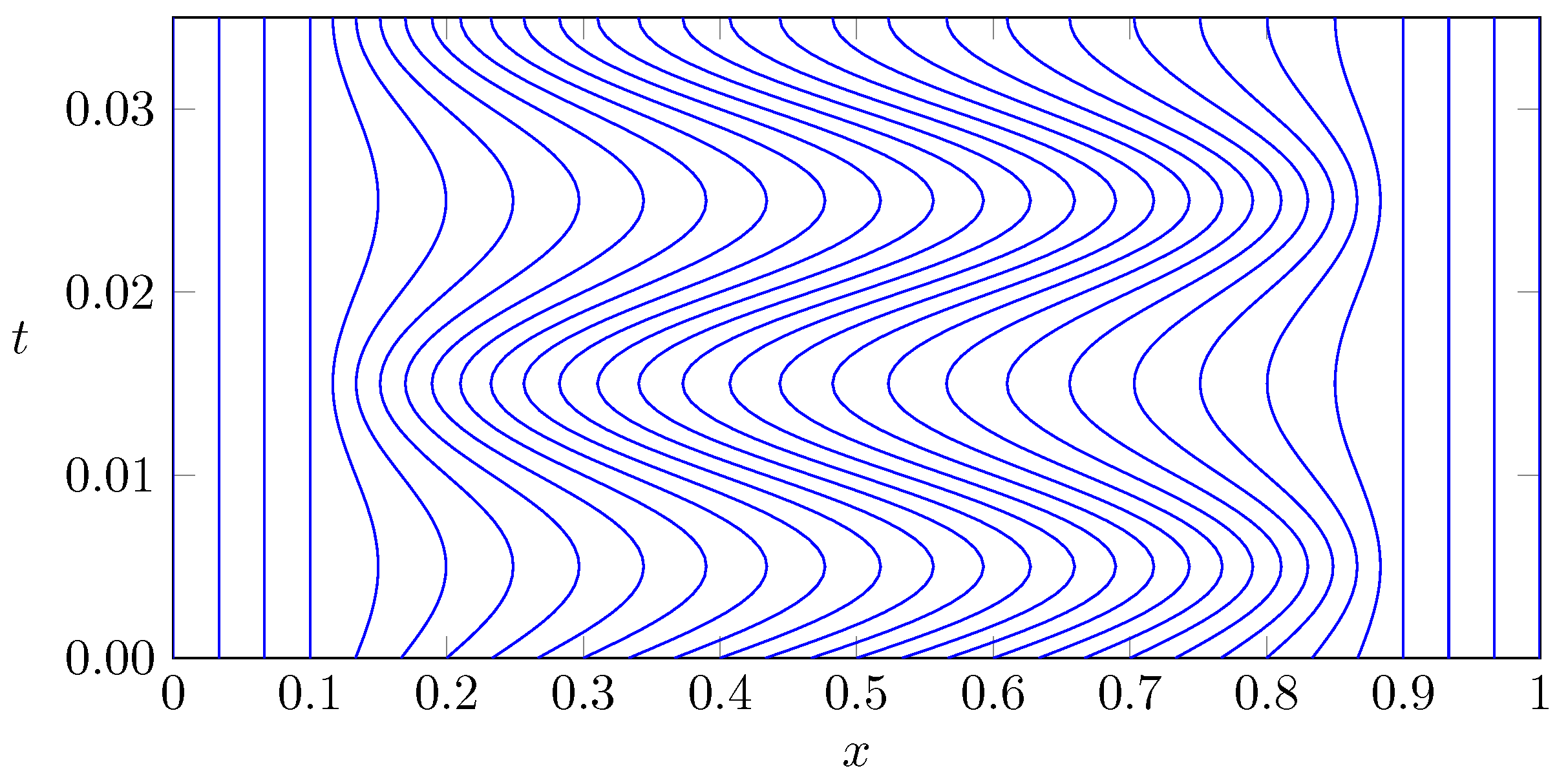
Figure 3 depicts the corresponding grid motion for an equidistant initial grid with
cells, a frequency of
and a confined region of grid movement bounded by
,
.
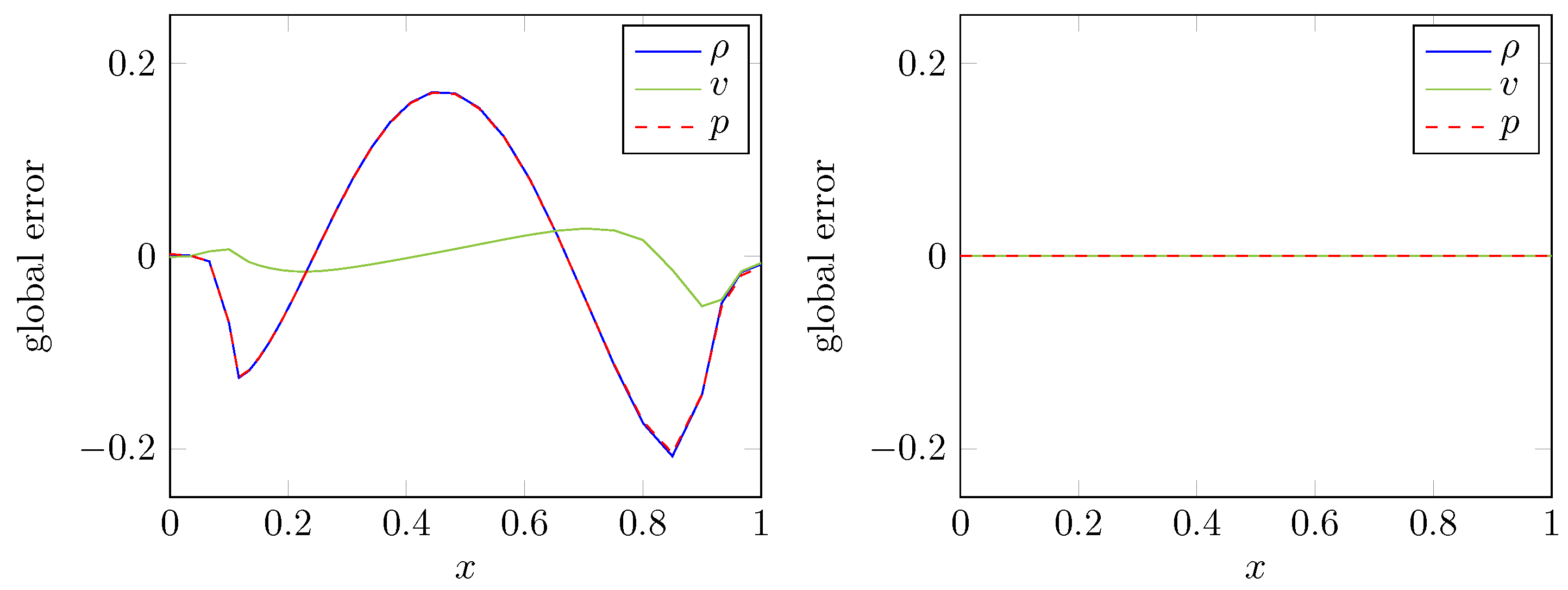
In order to illustrate the importance of calculating mesh velocities which are consistent with the GCL,
Figure 4 depicts the error with respect to density, velocity and pressure of the explicit Euler scheme applied to the fluid equations. More precisely, the right hand side of
Figure 4 shows the result for mesh velocities computed according to Equations (
59) and (
60) while the left hand side depicts the corresponding errors obtained by grid velocities determined from differentiation of Equations (
80) and (
81) with respect to
t. In the first case the constant initial state is preserved in accordance with the theoretical considerations while the second case does not lead to a numerical method consistent with the GCL.
Now we simulate this test case using the proposed MGARK scheme. In order to obtain a partitioning in fast and slow components, we consider the autonomous coupled system composed of the fluid variables as the fast components and the grid points as well as the time variable as slow components. Therefore, the grid motion given in Equations (
80) and (
81) is not prescribed exactly but provides a differential equation for the slow components of the coupled system. The slow components are hence evolved according to
starting from a given initial state
. Due to the ALE formulation Equation (
56) of the fluid equations, the fast components
are given by the products of the cell averages of the conservative fluid variables with the corresponding cell volumes. By the construction just described, the slow components are given by
and the coupling between these subsystems now takes the form
and
, which shows that the evolution of slow components is actually independent of the fast ones in this case.
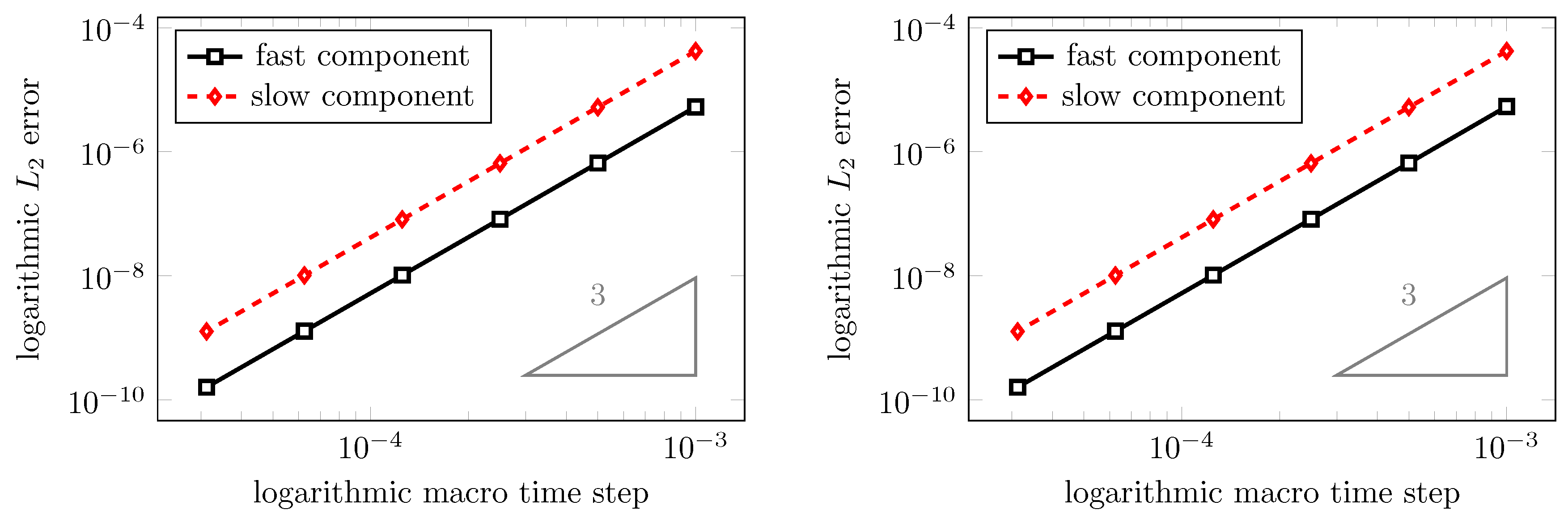
Figure 5 depicts the experimental order of convergence obtained by two different choices of base methods. The results on the left hand side are obtained by choosing the IMEXRKCB3c explicit/implicit schemes (
78) and (
79), i.e., the explicit third order scheme for the fast fluid component and the implicit third order scheme for the slow mesh movement component together with coupling conditions as given in Corollary 3. The right hand side shows the results obtained when replacing the explicit IMEXRKCB3c scheme with first order explicit Euler scheme for the fluid equations and setting all coupling coefficients to zero.
First of all, we observe that the chosen coupling strategies lead to an experimentally obtained convergence of third order. Though at first sight, it is striking that a global convergence of third order is also obtained using a fluid time discretization of only first order, we recall that our GCL-consistent MGARK scheme does not produce any disturbances of the constant fluid state, independent of the order of the fast base method. Hence, the global error is only determined by the slow base method which approximately determines the grid positions. Thus, the slow method solely determines the order of the coupled scheme in this case. However, in general, the accuracy of the coupled scheme reduces to first order if one of the base methods is only of first order.
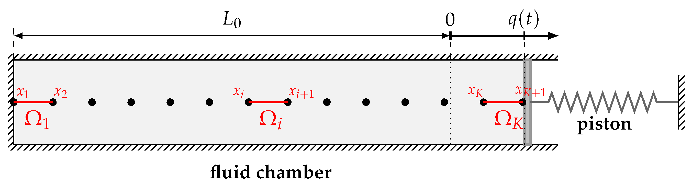
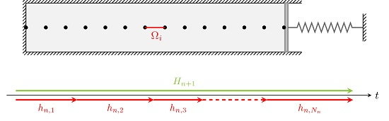
4.2. The One-Dimensional Piston Problem
The interaction between a piston which is attached to a spring and an inviscid fluid which is contained in a chamber is a classical test case in the context of fluid–structure interaction [
33,
34]. The coupled piston problem and its one-dimensional set-up are illustrated in
Figure 6.
In the mathematical formulation, the fluid is described by the one-dimensional inviscid Euler equations while the displacement of the piston is modelled by an undamped harmonic oscillator. In non-dimensional form we obtain a coupled system of the fluid equations given by
with
where
and
p denote density, velocity, specific total energy and pressure of the fluid, respectively, while
γ denotes the adiabatic coefficient, and the structure model for the piston displacement
given by
where the parameters in this non-dimensional formulation correspond to the mass
m and the stiffness
k of the spring as well as the cross-sectional area
A of the piston as well as its initial displacement
and velocity
. The piston displacement determines the length of the time-dependent fluid domain
according to
This domain is discretized by a constant number of grid cells, cf.,
Figure 6. Let
denote the grid points such that
. The influence of the fluid subsystem on the structure subsystem is given by the difference of the fluid pressure
acting on the piston at the fluid-structure interface, i.e., the right boundary of the fluid domain and the ambient pressure
.
The specific setting of the piston parameters
and
and the initial length
of the fluid domain as well as the initially constant fluid variables
,
,
and the initial piston displacement
and velocity
, which have been used in this test case are summarized in
Table 1.
We may now take a closer look at the difference in time scales for the fluid and structure subsystems in this set-up. The characteristic time scale of a fluid is given by the time needed by a pressure wave to traverse the chamber, i.e.,
where
c denotes the sound speed. For the values given in
Table 1 we obtain
.
The characteristic time scale of the structure is determined by the oscillation period, i.e.,
whereby we obtain
for the values in
Table 1.
The one-dimensional Euler equations in ALE formulation are then discretized by a finite volume method which yields
for interior grid cells, using a suitable numerical flux function
. At the two boundaries of
given by the grid points
and
, boundary conditions are required. As there is no movement of fluid particles through the boundaries of the fluid chamber (no-slip conditions), we demand that at the boundaries, the fluid moves with the same velocity as the corresponding boundary grid point. Suitable boundary conditions may be posed either as strong or as weak boundary conditions. Strong boundary conditions usually modify the numerical solution in a suitable way in order to satisfy the no-slip conditions. Weak boundary conditions usually modify the numerical flux in a suitable way. In comparison to strong boundary conditions, weak boundary conditions often lead to an improved convergence speed regarding iterative solvers and may also lead to an improved robustness, see [
35,
36,
37]. Concerning weak boundary conditions, both weak prescribed and weak Riemann approaches are common. In this work, we use the weak prescribed approach, i.e., the boundary fluxes are explicitly prescribed according to
with
For all of our numerical tests, we initially chose an equidistant discretization of the fluid chamber consisting of 100 finite volume cells and the numerical flux function
is given by the well known Lax-Friedrichs flux. The nonlinear systems of equations within the implicit stages of the RK scheme applied to the structure component (see Equation (
77)) are solved using a Newton-Krylov scheme. In order to introduce non-uniformity into this test case, the deformation of the fluid domain by the piston movement is transferred to the individual grid points in a non-uniform manner. In this set-up, the spatial grid is only equidistant at those time levels where the piston achieves its initial maximal displacement. In general, the computational grid is compressed near the piston. The results depicted in
Figure 7,
Figure 8 and
Figure 9 are obtained by adaptive determination of time step sizes for both macro and micro steps according to the strategies described in
Section 3.4, i.e., solely based on embedded error control. The parameters for time adaptivity are set to
,
,
for both micro and macro step sizes, and
for the macro step sizes as well as
for the micro step sizes. The simulation is carried out until the final time
.
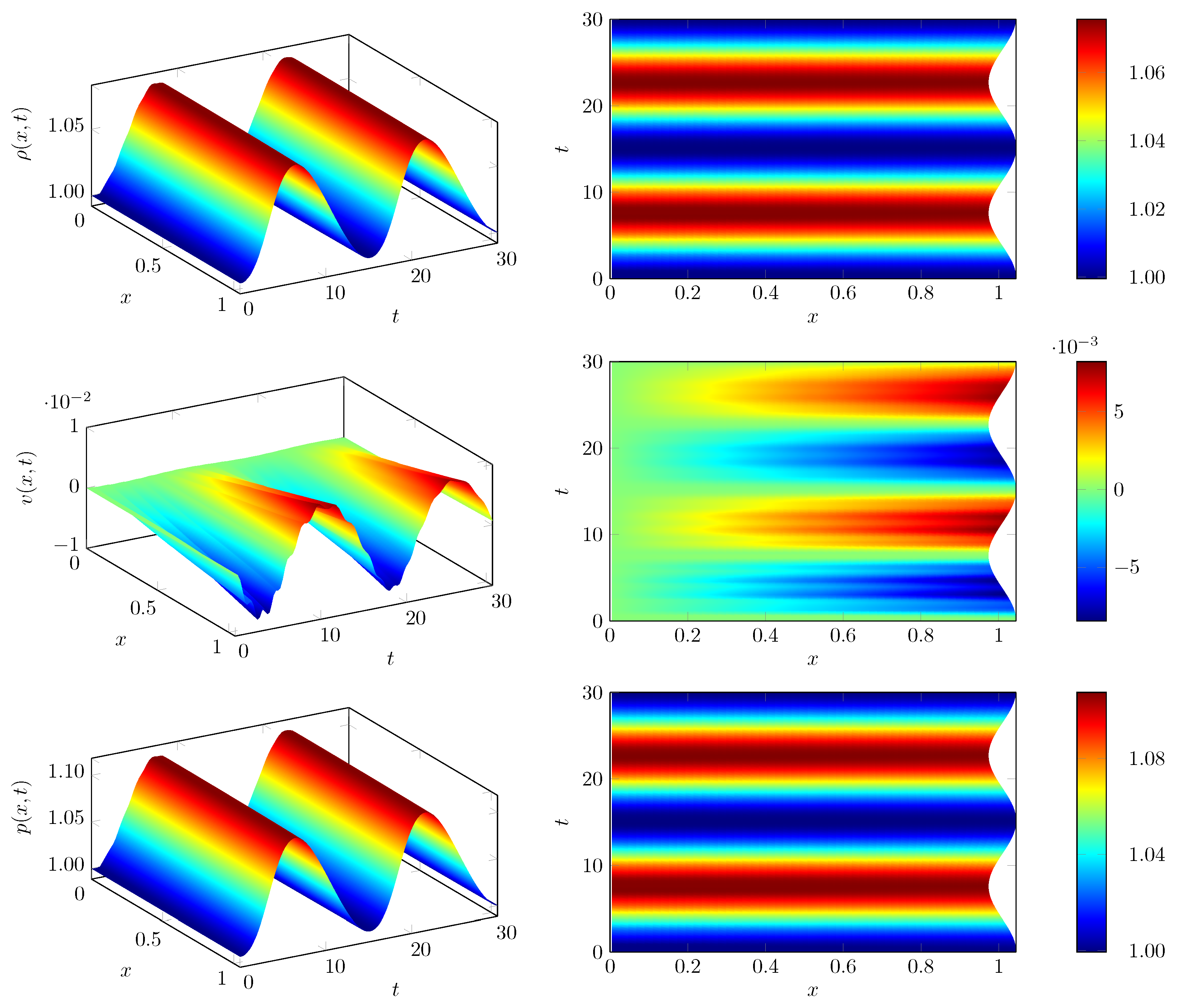
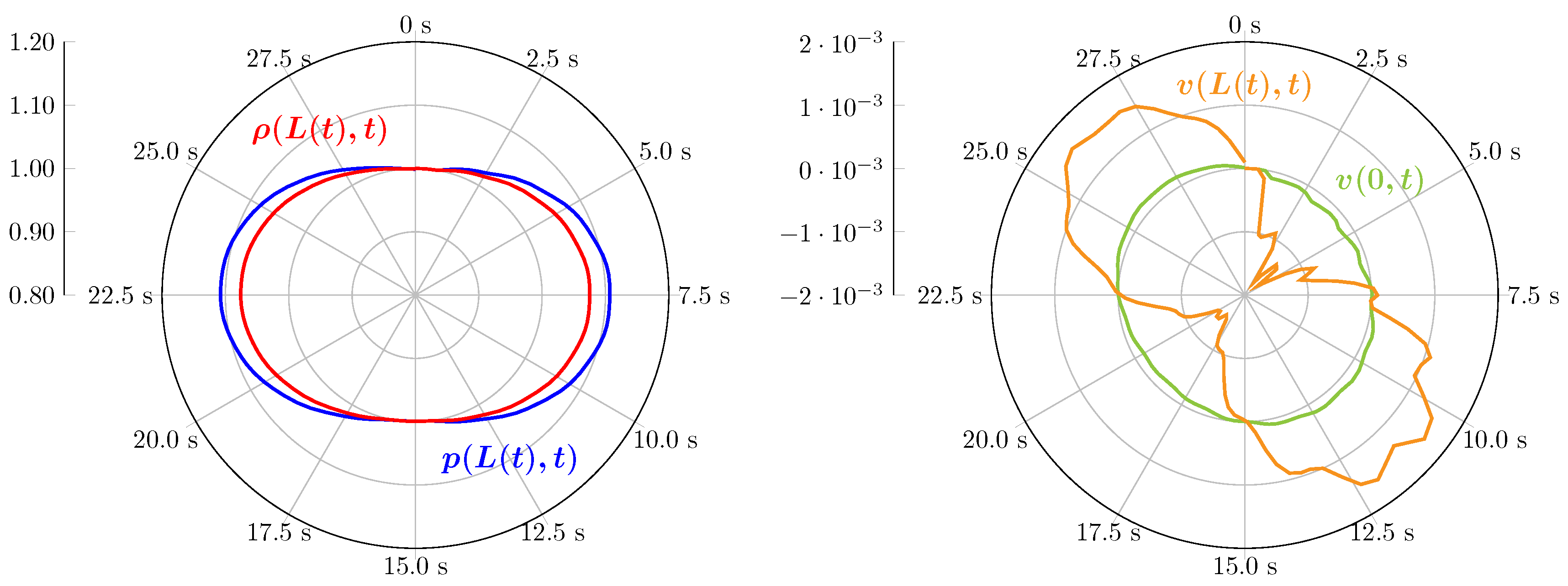
Figure 7 and
Figure 8 show the numerical results for the MGARK scheme based on the explicit Heun scheme for the fluid and the implicit trapezoidal rule for the structure. The coupling procedure is given by Choice B in Corollary 2. In the representations on the right hand side of
Figure 7, the piston movement at the right chamber boundary is visible as well.
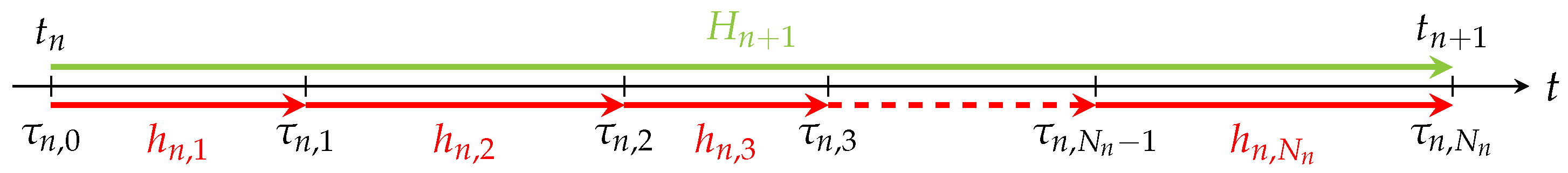
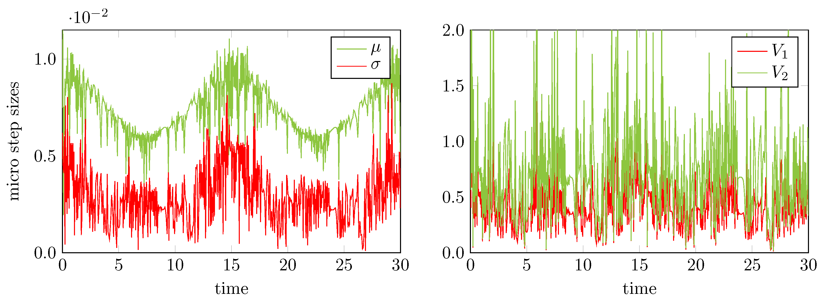
Now we would like to pay more attention to our strategy to allow for adaptive non-constant micro step sizes within one macro step. In this regard,
Figure 9 collects the statistics of the computed macro and micro step sizes. For the micro step sizes, the left part of
Figure 9 shows the time evolution of the mean value
μ and the standard deviation
σ calculated as
for
. Herein, the last micro step size of each macro step usually will be suitably shortened in order to add up to the macro step size, see Algorithm 4, line 8 and is hence not included into the calculation of the statistics. The coefficients of variation
and
relate the standard deviation as well as the maximum deviation to the mean value, i.e.
Hence, from these coefficients we obtain a measure of the extend of variability in relation to the mean.
As shown by the results on the right hand side of
Figure 9, there are time sections with significant variability of the micro step sizes, i.e., there are sections with
and sections with
. Thus, the application of variable micro step sizes instead of constant ones is justified for this test case. A multirate scheme using constant micro step sizes might have used the smallest micro step size to comply with the given error tolerances which would have led to a larger amount of micro steps per macro step compared to the adaptive choice of micro steps. For the time sections with higher coefficients of variation this means a higher computational effort and thus a lower efficiency compared to the adaptive case.
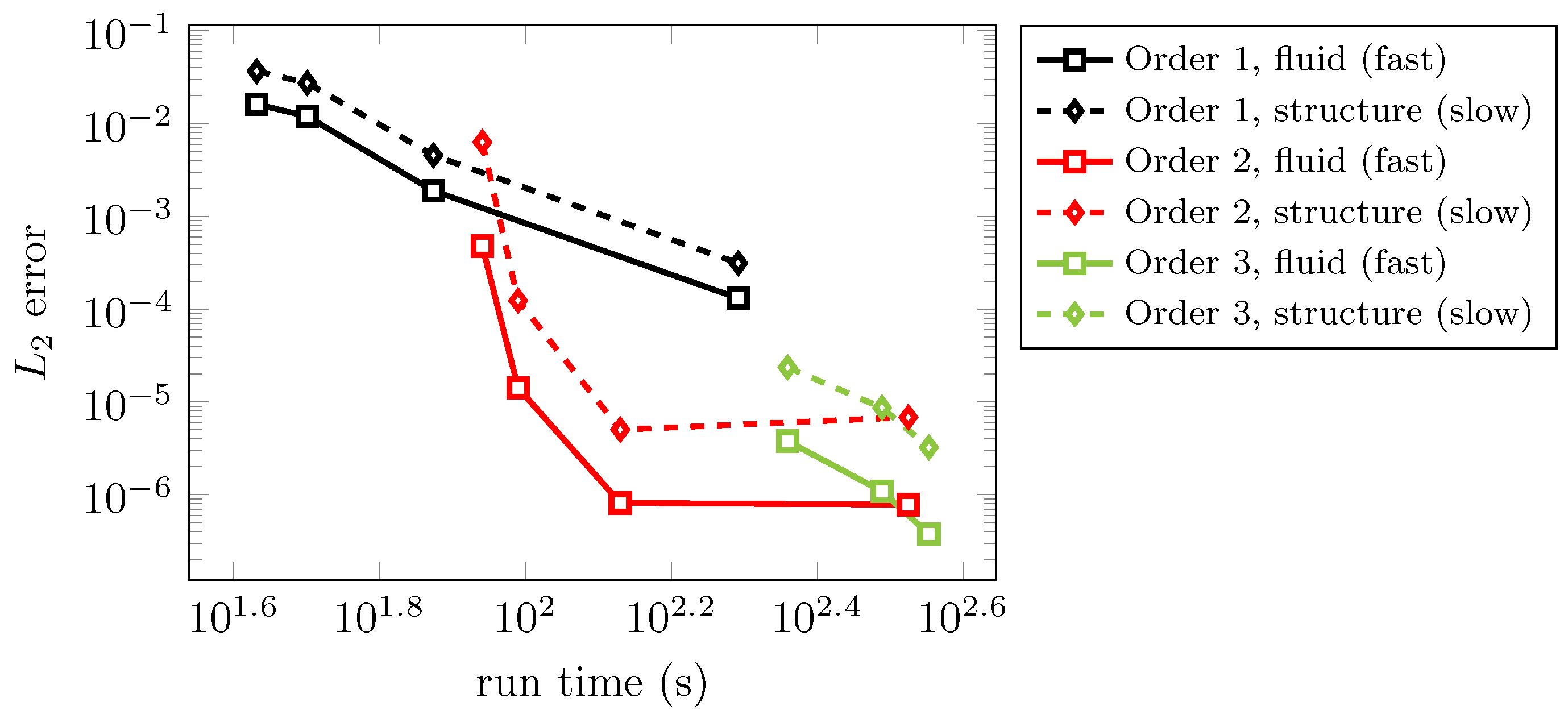
In
Figure 10, an efficiency study regarding numerical error versus CPU time is depicted comparing the described MGARK schemes up to third order. Computations were carried out for the explicit Euler method coupled with the implicit Euler method and coupling coefficients set to zero (order 1), the explicit Heun scheme coupled with implicit trapezoidal scheme and second order coupling coefficients according to Corollary 2, choice B, and the IMEXRKCB3c base methods with third order coupling according to Corollary 3.
A spatial discretization of 100 FV cells and a final time of
has been used in all test cases. The computations were carried out for different macro step sizes. During each computation, the macro step size was held constant while the micro step sizes were chosen with respect to the Courant-Friedrichs-Lewy (CFL) condition, with a CFL-number of
, i.e., according the error-controlled approach described in
Section 3.4. In order to compute the numerical error depicted in
Figure 10, a reference solution was calculated using the 3rd order explicit IMEXRKCB3c scheme to solve the fluid–structure system as a whole in a monolithic manner with a suitably small time step size and without the use of different step sizes for the subsystems.
We remark that the reference solution is obtained on the same spatial grid as the numerical simulations. Therefore, we in fact measure the time integration error of the MGARK variants applied to the semi-discrete system which is generated by finite volume space discretization Equation (
82) of first order. As the focus of this work is on time integration, we expect this to be a reasonable measure for the quality of the time integration process. Of course, the full discretization error, which may be measured with respect to a reference solution on a refined spatial grid, will be affected by both spatial discretization method and time integration scheme.
We may observe that the second order coupled time integration is most efficient for moderate to small tolerances in the range of about to . For even smaller tolerances, the third order coupled procedure starts to become efficient for this specific test case.
An efficiency study regarding run time and accuracy was carried out for the 2nd order MGARK scheme described above. The results are summarized in
Table 2 and
Table 3 on page 30. Again, we approximated the error using a reference solution obtained by an explicit 3rd order in time monolithic approach using a suitably small constant time step size. Within
Table 2, the macro step size is denoted by
H and is held constant,
N denotes the number of micro steps per macro step,
respectively
denote the error of the fast respectively slow system component measured in
norm,
is the average number of micro steps per macro step in case of a micro step size adaptive approach and TOL denotes the relative and absolute tolerances in case of error-controlled adaptivity. The remaining parameters needed by error-controlled adaptivity were always set to
,
and
for both micro and macro step sizes.
For the computations with an error-controlled micro step size, an initial step size of
has been used. A dash indicates that the scheme diverged for the specified settings. The right part of
Table 3 was computed using the minimum micro step size given by comparing the error-controlled approach to a CFL-compliant step size computation with a CFL number of 0.9.
We observe that the best error achieved with constant macro and micro step sizes is undercut by the error obtained with both of the fully-adaptive approaches (i.e., adaptive macro step sizes and adaptive micro step sizes, see
Table 3) with suitably small tolerances. At the same time the fully-adaptive approaches also perform better regarding run time. In addition to the results shown in
Figure 9 these results demonstrate the efficiency of our approach to time adaptive MGARK schemes and show its potential to be successfully applied to more sophisticated real-world problems.


 ) denote zero entries while the red ones (
  ) denote entries required to be non-zero in agreement with our strategy of enforcing the GCL and the green-colored blocks (
  ) symbolize arbitrary entries.
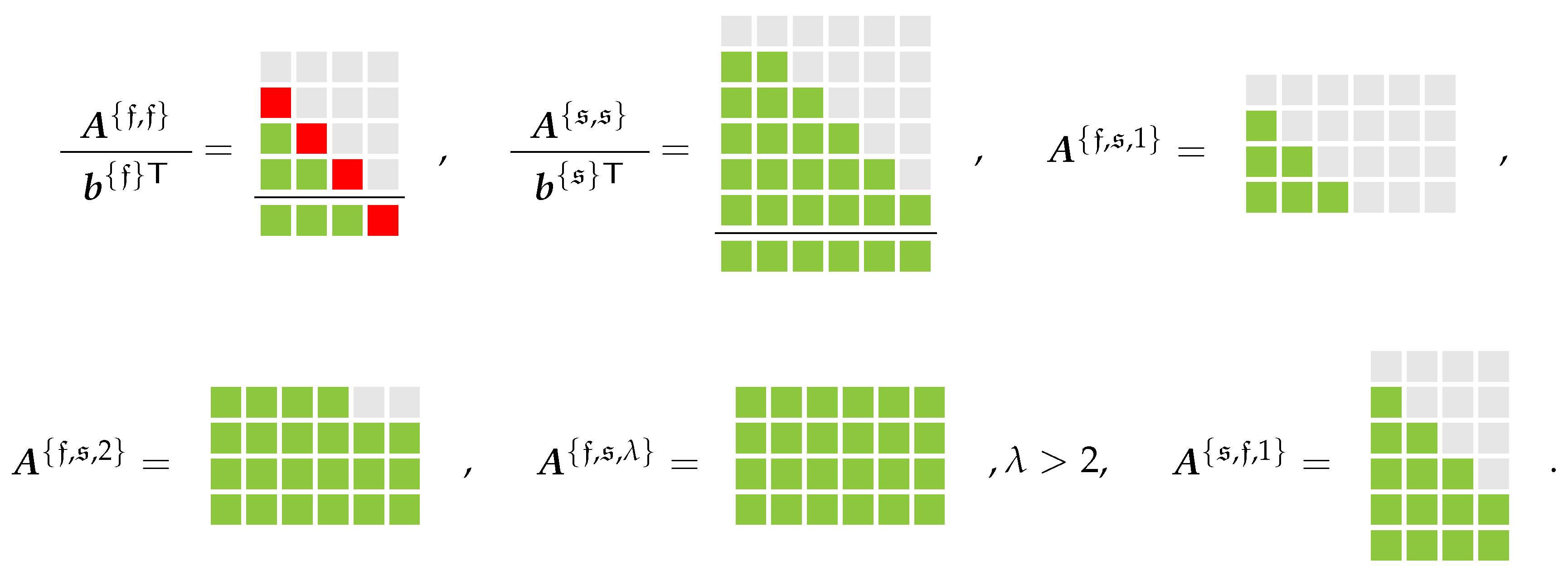


