
Direct Entry Minimal Path UAV Loitering Path Planning †


Department of Mechanical Engineering, Russ College of Engineering and Technology, Ohio University, Athens, OH 45701, USA
*
Author to whom correspondence should be addressed.
†
This paper is based on the results presented in Development of an Area of Interest Extended Coverage Loitering Path Planner. In Proceedings of the AIAA Infotech@Aerospace, AIAA SciTech Forum, San Diego, CA, USA, 4–8 January 2016.
Aerospace 2017, 4(2), 23; https://doi.org/10.3390/aerospace4020023
Submission received: 11 March 2017
/
Revised: 31 March 2017
/
Accepted: 4 April 2017
/
Published: 18 April 2017
(This article belongs to the Collection Unmanned Aerial Systems)
Abstract
:Fixed Wing Unmanned Aerial Vehicles (UAVs) performing Intelligence, Surveillance and Reconnaissance (ISR) typically fly over Areas of Interest (AOIs) to collect sensor data of the ground from the air. If needed, the traditional method of extending sensor collection time is to loiter or turn circularly around the center of an AOI. Current Autopilot systems on small UAVs can be limited in their feature set and typically follow a waypoint chain system that allows for loitering, but requires that the center of the AOI to be traversed which may produce unwanted turns outside of the AOI before entering the loiter. An investigation was performed to compare the current loitering techniques against two novel smart loitering methods. The first method investigated, Tangential Loitering Path Planner (TLPP), utilized paths tangential to the AOIs to enter and exit efficiently, eliminating unnecessary turns outside of the AOI. The second method, Least Distance Loitering Path Planner (LDLPP), utilized four unique flight maneuvers that reduce transit distances while eliminating unnecessary turns outside of the AOI present in the TLPP method. Simulation results concluded that the Smart Loitering Methods provide better AOI coverage during six mission scenarios. It was also determined that the LDLPP method spends less time in transit between AOIs. The reduction in required transit time could be used for surveying additional AOIs.
1. Introduction
The development of Fixed Wing Unmanned Aerial Vehicles (UAVs) as surveillance tools has grown exponentially in remote sensing applications [1,2]. The militarization of remote sensing UAVs has been to said reduce risk and workload on soldiers as well as improve reconnaissance efforts [3]. Small (Group 1) hand launched UAVs, such as the RQ-11 Raven [4,5], are limited to flying shorter duration missions compared to the large UAVs and therefore efficiency of remote sensing is paramount. Increasing the efficiency in path planning could potentially increase sensor coverage, which will be the primary focus of this paper.
Loitering, the act of circling an Area of Interest (AOI), is commonly used during remote sensing. Small UAV autopilots tend to initiate the loitering by flying directly through the center of the AOI, also known as the Point of Interest (POI), prior to circling [6,7,8,9].The Pixhawk autopilot, developed by 3D-Robotics [10], can be programmed for fixed wing aircraft is a commonly used autopilot that has this loitering feature. This loitering behavior will be referred to as the Fly Through method for the remainder of the paper. The loiter is programmed into the autopilot system as a number of waypoints that pass directly through the POI and circle around until an overlap with the AOI is accomplished, which is shown in Figure 1. While the Fly Through method allows the UAV to loiter, it requires an extra turn outside of the AOI, which could cause a loss in sensor coverage of the AOI.
In order to decrease the loss in sensor coverage while loitering, two novel loitering methods were investigated and compared against the Fly Through Method in simulation based on previous work [11]. The first method transits from one POI to another along a vector tangential to the POIs’ respective AOI edges. The second method transits along the vector connecting POIs and enters the loitering tangentially by executing a turn at the UAVs’ minimum turning radius. Both novel methods avoid a direct Fly Through, resulting in an increased sensor coverage and have the added benefit of reducing flight time. The path planning simulations were programmed so that the path was represented as a finite number of UAV waypoints, which could easily be implemented into current autopilot systems with little to no modification. The implementation of sending the generated waypoints to the autopilot is a possible area of future work.
1.1. Path Planning and Loitering
Path planning is the process of formulating a route that moves an entity from an initial state to a final state based on vehicle dynamics and navigational requirements [12]. The two common path planning methods that were examined were road map and pose-based methods. Road map path planning methods break down a solution space into a finite number of discrete segments. A desired mission optimization criterion is then used to select an optimal path in the solution space. Common road map methods include the Voronoi diagram [13] and cell decomposition [14]. Road map and cell decomposition methods were not found to be useful for the loitering simulations due to the main disadvantage of the methods being obstacle avoidance driven and not the shortest path. Pose-based path planning methods consist of generating a path that traverses a series of specified waypoints in space. Notable pose-based path planning methods include the Dubins and the Clothoid methods.
The Dubins pose-based path planning algorithm was developed by L.E. Dubins in 1957 [15] and uses a combination of circular arcs of a constant radius and straight line segments to generate a path. Arcs and straight path segments are then connected to each other via relevant tangent points to construct a full path. Grymin and Crassidis [16] applied the Dubins method to construct a flyable trajectory for a UAV tasked to navigate through a series of waypoints. In the study, a simplified aircraft model was constructed under the assumptions of constant velocity and turn radius. Karas [17] implemented the Dubins paradigm to model a two-dimensional fixed wing aircraft flight path.
Clothoid paths are similar to the Dubins method; however, they provide continuous arc paths instead of straight line segments. Using a Clothoid continuous curvature profile results in a gradual or ramp acceleration profile that may be easier for commonly used UAV platforms to follow. Wilburn [18] developed a three-dimensional UAV Clothoid trajectory generation algorithm that produced flyable paths of continuous curvature that ensured a command path that can be followed. The method presented by Wilburn [18] was developed as an extension of the three-dimensional Dubins and two-dimensional Clothoid methods. Shanmugavel [19] implemented the Clothoid method to generate safe and flyable flight paths for a cooperative group of UAVs tasked to arrive simultaneously on a target. Al Nuaimi [20] compared the differences between the Dubins and Clothoid methods. Simulations considered trajectory tracking control laws under various flight conditions. It was found that the Dubins path yielded increased tracking errors due to the discontinuous change in lateral command accelerations at the transition points between circular arcs and straight segments. However, accuracy of a UAV in following a command path is not considered a governing factor in maximizing the effectiveness of a loitering fixed wing UAV surveying an AOI. Since the accuracy of the UAVs’ flight path was not vital for the purpose of the proposed loitering path planner methods, Dubins was used to both simplify the algorithms and keep computational efforts at a minimum.
1.2. Dubins
In the work presented, a fixed wing aircraft flight path was modeled to fly to and survey a series of AOIs in a search space. Dubins arcs were used to expressed bank maneuvers and Dubins straight path segments were used to express forward paths in a constant direction. Bank maneuvers were modeled as curved paths with radii equal to the aircraft minimum turn radius at the aircraft cruise speed. A sampling rate of one second was used to calculate the flight path segments. Sampling the flight path at a one second rate ensured that computational efforts of the algorithm were kept to a minimum while maintaining the curvature needed to describe the flyable path.
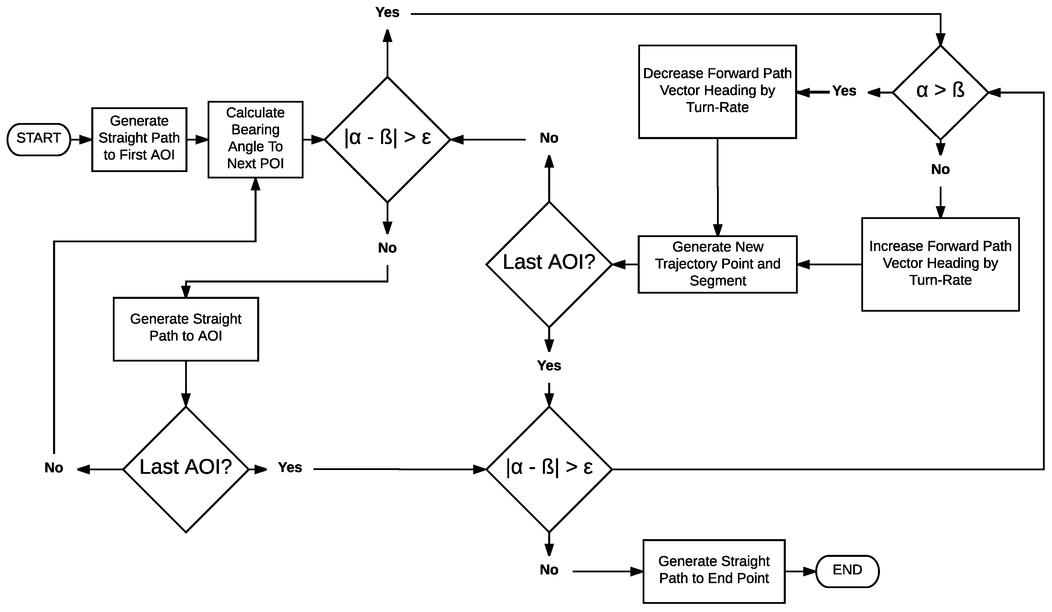
Flight paths generated using the Dubins method were achieved with an algorithm that produced a new trajectory point and path segment at each time step. The logical steps of the Dubins method are summarized in the flowchart shown in Figure 2, where each trajectory point calculated corresponded to the start and the end of a path segment. Segments that are expressed by a forward path velocity vector in the direction of the aircraft current heading angle , shown in Figure 3, where the bearing angle, , represented the angle between a consecutive POI relative to a current POI or location. The Dubins process is achieved by first determining a bearing angle to the first POI relative to the aircraft current position. Aircraft heading angle was then set equal to the bearing angle , as the aircraft was initially assumed to be inbound towards the first POI. Straight path segments were generated until the first POI was reached. Once the aircraft reached the first POI, the algorithm determined the difference between the aircraft current heading angle and the bearing angle to the next POI. The difference between angle and was compared to the aircraft turn-rate angle , which was the maximum angle that the aircraft could turn at each time step. If the difference between the angles was found to be larger than the turn-rate angle , the aircraft heading angle was adjusted by adding or subtracting the turn-rate angle . Aircraft heading was incrementally adjusted until the difference between the heading angle and bearing angle was smaller than the turn-rate angle . At this point, the aircraft was in a straight line path with the next POI and straight path segments were generated.
1.3. Loitering
Loitering flight paths are executed during UAV operation to satisfy or optimize mission or user defined objectives. Rathinam [7] applied loitering to idling flight between tasking, exploratory flight utilizing a surveying sensor payload, and as a safe state in the event of failure or divergence from mission objectives. Similarly, Alighanbari [6] discusses the way by which timing constraints for a multi-UAV mission visiting multiple pre-defined waypoints can be satisfied by loitering about waypoints, therefore optimizing the overall mission time.
Sujit [8] explored effectiveness with which loitering and straight line paths could be simulated based on several commonly used path planning algorithms with particular regard to cross-track error. While loitering flight paths have been investigated for application in various UAV missions, the effect of loitering flight path geometry optimization on overall mission performance has not yet been explored in detail and, thus, is the basis of the presented study.
2. UAV Flight Parameters
2.1. Path Planning
MATLAB, developed by MathWorks was used to model and analyze flight path simulations for a fixed wing aircraft using the two-dimensional Dubins [15] method to generate a flyable path. A pose-based Dubins path planning method was selected for this application where the waypoints represented the centers of the AOIs and the offset points for the loitering path entries and departures. The Dubins method was selected so the aircraft in flight behavior could be simplified and represented in a two-dimensional space using Dubins arcs and straight paths and has been implemented in UAV path planning previously [16,21,22]. Heading changes are described using Dubins arcs and straight paths using Dubins straight path segments.
2.2. UAV Sensors
In order to collect surveillance data from the AOIs, the internal payload and underbelly of the UAV will house a camera mounted on a one degree of freedom gimbal with a 74° Field of View (FOV). The nominal position of the camera was assumed to point directly downward providing a coverage area of 6638 m, seen in Figure 4a. When necessary, the camera would gimbal to either side of the UAV to maximize the AOI inside the camera’s FOV. Figure 4b shows the maximum gimbal angle of 25, measured from the vertical. At the gimbal angle of 25, the FOV captures a coverage area of 51,223 m.
3. Loitering Path Planner Methods
Three loitering methods were developed and simulated in the following section. The Fly Through loitering path planner method required the aircraft to fly directly through the center of the AOI before turning into a loiter [6,7,8,9]. Turning into the loiter resulted in a loss of coverage due to the aircraft traveling outside of the capable surveillance range of the gimballed camera system. In order to eliminate the need to fly outside of the surveillance range, the Tangential Loitering Path Planner (TLPP) was developed. The TLPP method required the aircraft to depart and enter AOIs tangentially such that the aircraft approached the AOI perimeter and entered the loiter immediately for maximized AOI coverage. Finally, the Least Distance Loitering Path Planner (LDLPP) was developed to reduce the transit distance and overall mission time by flying a path directly from POI to POI. Upon approaching the AOI perimeter, a loiter entry turn was executed, placing the aircraft on the AOI perimeter while the loiter departure turn placed the aircraft on a direct path in the direction of the next POI. Simulated flight data for AOI coverage and mission time were collected and compared for each of the three methods discussed.
3.1. Fly through Loitering Path Planner
The Fly Through loitering path planning algorithm established a basis of the underlying functions that will be utilized to develop UAV flight paths. The initial path planner was based on algorithms present in the Pixhawk autopilot system that produces a path that flies through the radius threshold of a POI and then begins to loiter. Modeling of a Fly Through loiter was achieved using the Dubins method that directed an aircraft to a POI and then began the loitering process at the aircraft’s maximum turn rate. Once a pre-determined number of loiters had been performed, a path was then planned to the next POI or home if all POIs had been visited.
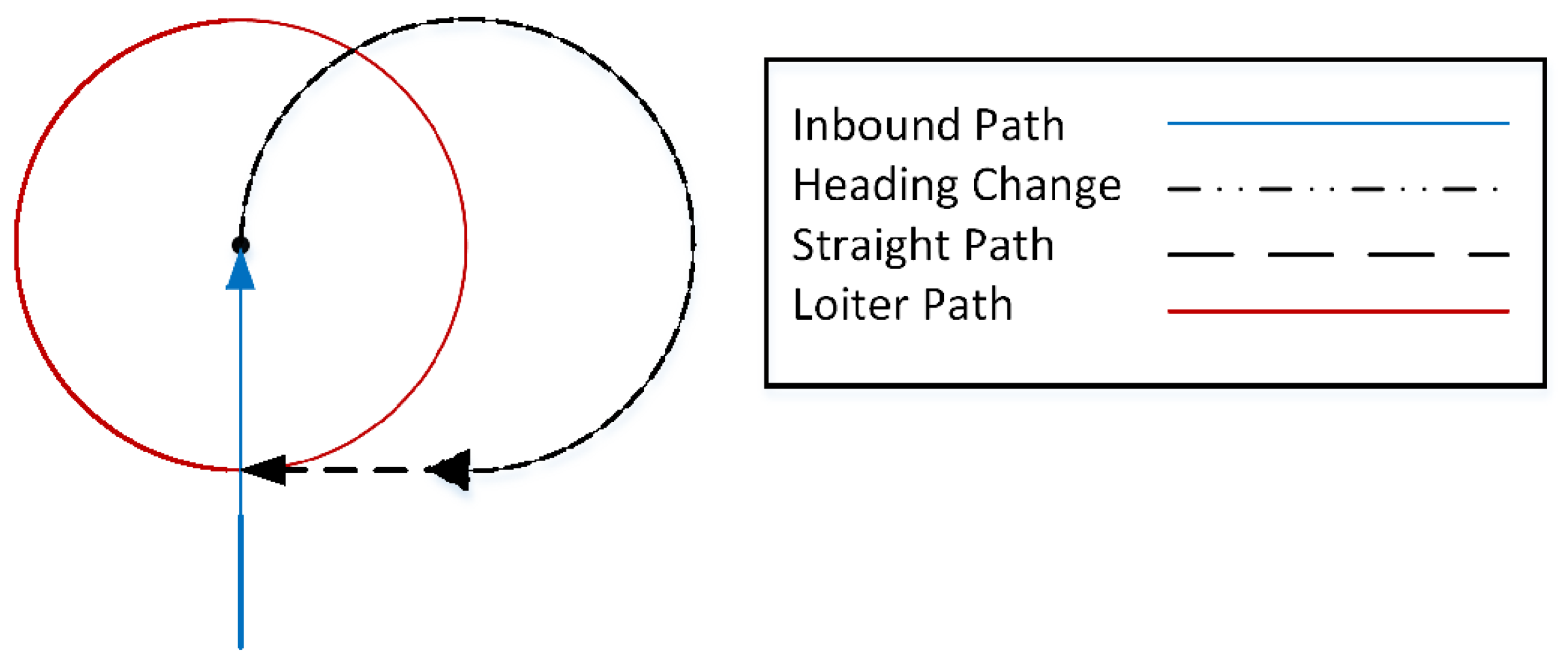
The initial iteration of a loitering path planning method was designed to increase sensor coverage by performing a loiter path around the center of the AOI. The loitering path planning was achieved by tasking the aircraft to fly through the center of the AOI first, increase or decrease headings to perform three quarters of a full turn and then fly a straight path to enter a loiter path, as illustrated in Figure 5.
The Fly Through path planner process began by determining the required bearing angle between the current position of the aircraft to the center of the first AOI. Straight path segments were then generated until the aircraft reached the center of the first AOI. Once the aircraft has reached the AOI, the algorithm determined whether it will enter into a clockwise (CW) or counterclockwise (CCW) loiter path direction around the AOI. The entry direction was determined by checking the position of the next AOI relative to the current AOI and determining if exiting the loiter path in a CW or CCW is in the direction of the next AOI. The direction check ensured that the heading changes required to reach the next AOI are minimized upon completing a loiter path. The aircraft entered the loiter path by changing its heading, in the determined CW or CCW direction, until it was in line with an offset point from the center of the AOI. The offset point was located at a distance equivalent to the minimum turn radius of the aircraft and was located along the aircraft initial inbound path to the AOI. To reach this point, the aircraft had to perform three quarters of a full loiter path for its heading to be in line with the offset point. A straight path was then generated to reach the offset point and was followed by the loiter path around the AOI. Upon completing the loiter path, the aircraft was in the same heading in which it entered. The heading is then adjusted accordingly until the aircraft is in a straight line path with the center of the next AOI. This iterative process continued until all AOIs were visited and the aircraft reached the end point. An example of the Fly Through loitering path can be seen in Figure 6. What can be seen is that a straight path is first generated to the center of AOI 1. The path then enters into a CW heading change until it completes three quarters of a full turn, which is then followed by a straight path. The straight path is continued until it reaches the entry point of the loiter path. The CW loiter path was then preformed and at this point the aircraft is in a straight line with the center of AOI 2. The path continues in this fashion until the path reaches the end point.
3.2. Tangential Loitering Path Planner
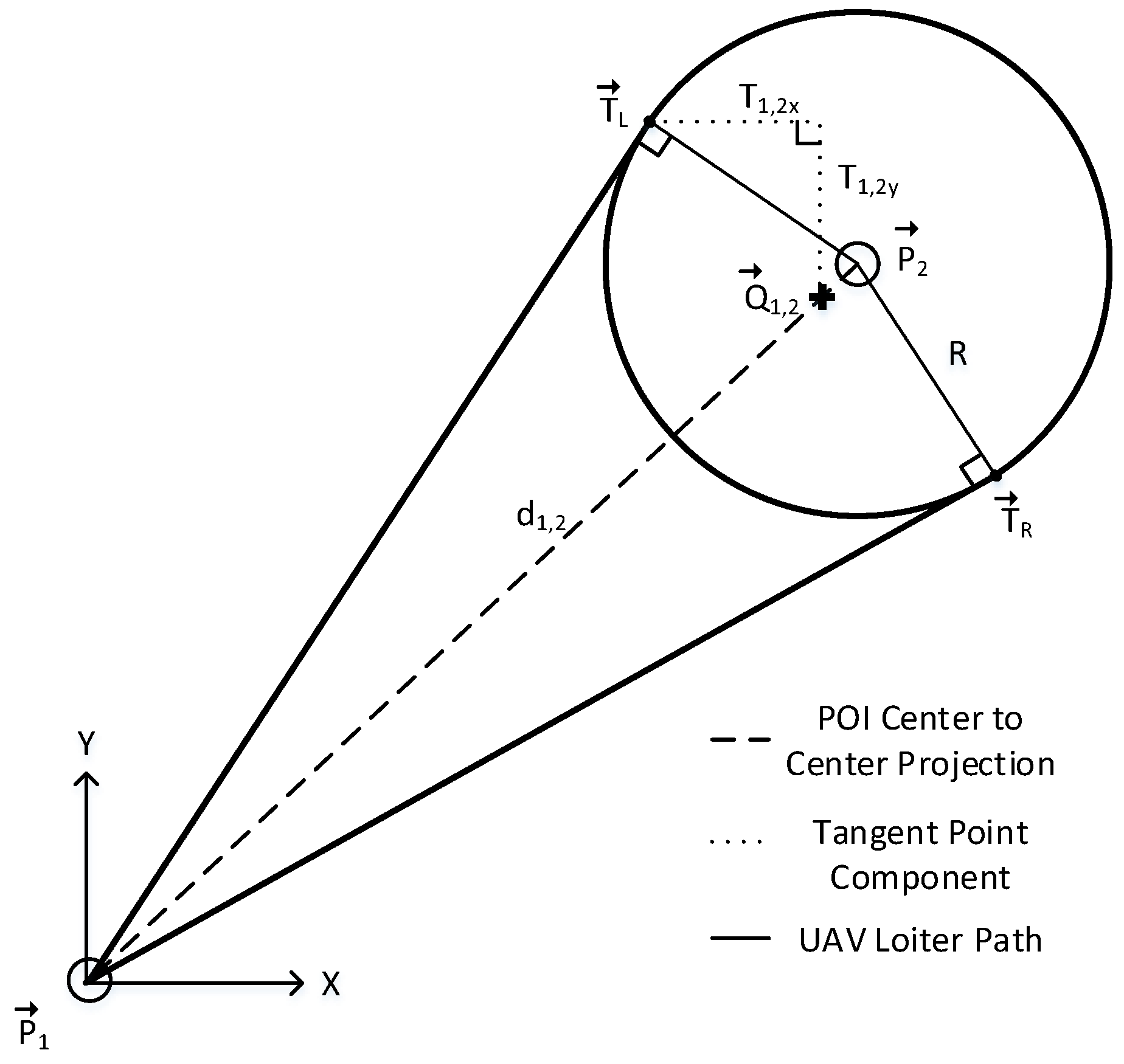
A secondary loitering path planning method called the Tangential Loitering Path Planner (TLPP) was sought to enable an aircraft to directly enter and depart a loiter path via tangent points. TLPP was an extension of the fly through and loiter path planner; however, it eliminated the necessity to travel an additional path to enter the loiter path. The algorithm first determined whether to enter the first AOI in a CW of CCW direction. This was determined in the same manner as the fly through and loiter path planner by checking the position of the next AOI relative to the current AOI. Once the direction was established, the algorithm calculated the coordinates of a point that was both the offset from the AOI and tangent to the aircrafts current position and allowed the aircraft to enter the path in the intended CW or CCW direction and can be seen illustrated in Figure 7. This figure shows the starting point as POI 1 and the center of the AOI as POI 2 with the AOI loiter path at a radius of R. The tangent point to the left can then be seen as and the tangent point to the right can be seen as . The process by which the tangent points are determined is summarized in Equation (1) through Equation (7).
Following with the POI configuration presented in Figure 7, the position vector of the POIs, and , are expressed in the form shown in Equation (1):
The first step in determining the tangential entry points along the AOI perimeter was to calculate the difference between and , for which the operation is shown in Equation (2):
where is the 2D position vector of POI 1 and is the 2D position vector of POI 2. Taking the difference between position vectors, and , allowed for the determination of tangent points relative to the positions of both POIs in succeeding steps. Next, the Euclidean distance between and was found by taking the square root of the dot product, seen in Equations (3) and (4):
yields the distance between the two POIs, where is the distance from and squared. In order to obtain the positions of the left and right tangential entry points on the perimeter of AOI 2 from the direction POI 1, a geometric reference point, , was established between POI 1 and POI 2 via Equation (5).
The displacement required to find the tangent point on the AOI perimeter from the direction of POI 1, , was then calculated in Equation (6):
where R is the AOI radius and r is the turning radius of the UAV. Lastly, the position of the left and right tangential entry points, and , were calculated using Equation (7), wherein the displacement was added to and subtracted from the established geometric reference point for the right and left tangent points, respectively. The left and right tangent points are symmetric about the line .
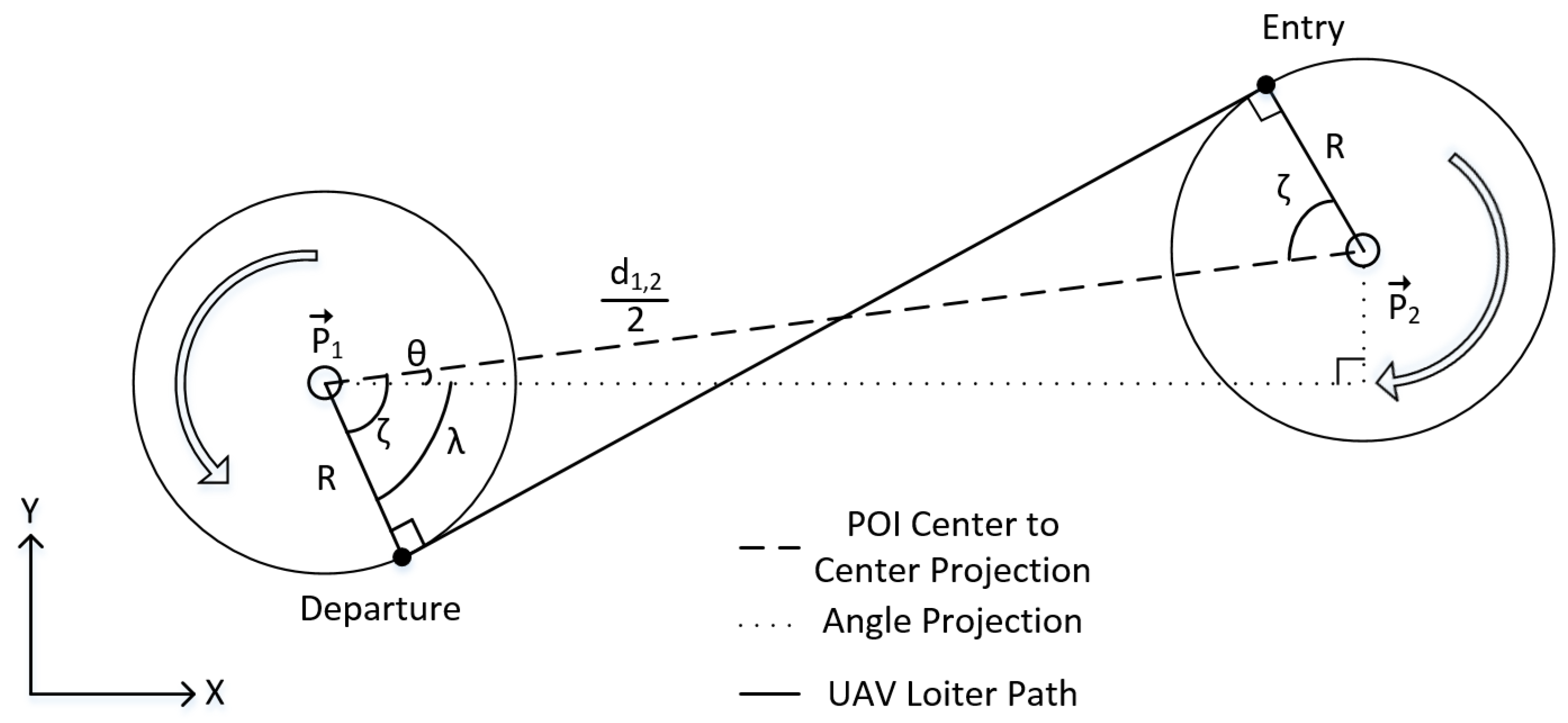
where is a geometric reference point relative to and , and is the displacement measured from to tangent of AOI relative to and . The bearing angle required to reach the tangent point was calculated using the current heading of the aircraft assuming that it was initially inbound to the center of the AOI. Straight path segments were then generated to reach this point followed by a loiter path in the intended CW or CCW direction. Upon completing the loiter path, the algorithm calculated the set of inner tangent points between the current loiter path and the loiter path around the next AOI. One of the points in the set represented the departure point along the current loiter path direction and the other represents the entry point along the next loiter path direction. Assigning the departure point in this way allowed for additional coverage time of the current AOI before proceeding in a straight path to the next loiter path. An example of the inner tangent departure calculation is presented in Figure 8 in which the aircraft is departing from the current loiter path around POI 1 in a CCW direction and entering the next loiter path around POI 2 in a CW direction.
The departure and entry point are determined by executing the following steps in reference to the POI geometry presented in Figure 8, wherein the 2D position vectors of POI 1 and 2 are expressed as before in Equation (1). Similarly, the distance between the two POIs is found using Equations (2)–(4). The bearing angle off of the horizontal between between POI 1 and 2, , was determined by taking the inverse tangent of the absolute value of the Y and X values of . The calculation of is shown in Equation (8) and the geometry is represented by angle projection lines in Figure 8:
where is the difference between position vectors and . The departure angle between and r about point produced a path that bisected the line , yielding two similar right triangles and an equivalent entry angle into the loiter about . From the right triangle geometry that is consistent with tangential entry and departure, the tangential departure/entry angle was calculated in Equation (9):
where R is the AOI radius and is the distance between POI 1 and POI 2. The sum of these two angles, and is taken in Equation (10), which yielded the tangential departure/entry angle from the horizontal, as shown in Figure 8:
where is the tangential departure/entry angle from POI 1 to POI 2 and is the bearing angle between POI 1 and POI 2. With the tangential departure/entry angle from the horizontal, , the position of departure and entry points from the respective POI were determined through Equations (11) and (12):
where is the X coordinate of POI 1, is the Y coordinate of POI 1, is the X coordinate of POI 2, is the Y coordinate of POI 2, R is the radius of AOI, and is the tangential departure/entry angle off of horizontal between POI 1 and POI 2. The tangential loitering path method was capable of successfully generating paths for an aircraft that avoided extra or wide turns associated with the Fly Through loitering method. A key feature of the TLPP was that the aircraft entered the next loiter path in the opposite CW or CCW direction from the previous loiter path, meaning that the determination of CW or CCW loiter path entry was only necessary for the first AOI. This iterative process was repeated until all AOIs were visited and the aircraft reached the end point. An example of the TLPP is shown in Figure 9 for five POIs. Note that the TLPP did not have any extra or unnecessary turning outside of the AOI that was present in the Fly Through method. The tangential point to the first loiter path was calculated and is presented in Figure 9 as the green point to the lower right of the center of AOI 1. The path then proceeded into a CCW loiter path and, upon completion, followed an additional loiter path denoted in red to the departure point at the upper right of AOI 1. At this point, the heading was in a tangential straight path with the next AOI, which was slotted to execute a CW loiter. This process of tangential entry and departure was repeated until the vehicle reached the end point. TLPP was found to be significantly more effective than that of the Fly Through and loiter method with both reduced overall mission times and increased AOI coverage. Not only did the TLPP method avoid the additional path needed in the Fly Though method, but it was much simpler in terms of navigation and will work best with existing autopilot systems that operate off waypoint navigation.
3.3. Least Distance Loitering Path Planner
Although TLPP yielded smooth entry and departure maneuvers that increased sensor coverage while in proximity of an AOI, it did not follow the shortest or most direct route from one AOI to another.The shortest path between AOIs would simply be to fly along the vector connecting each AOI. In order to further optimize sensor coverage and reduce overall mission duration, a third solution was developed that incorporated both smart loiter entry and departure maneuvers as well as a direct flight path between AOIs, termed the Least Distance Loitering Path Planner (LDLPP).
LDLPP consisted of four fundamental maneuvers that ultimately allowed for the overall reduction of transit distances between AOIs. The four maneuvers consisted of transit between AOIs, curved loiter entry, loiter, and curved loiter departure. LDLPP repeated the four fundamental maneuvers in order until the vehicle reached the desired end point. It is important to note that the departure maneuver placed the vehicle on a path directly in line with the next POI rather than on target with the tangent of the next AOI as in the TLPP method.
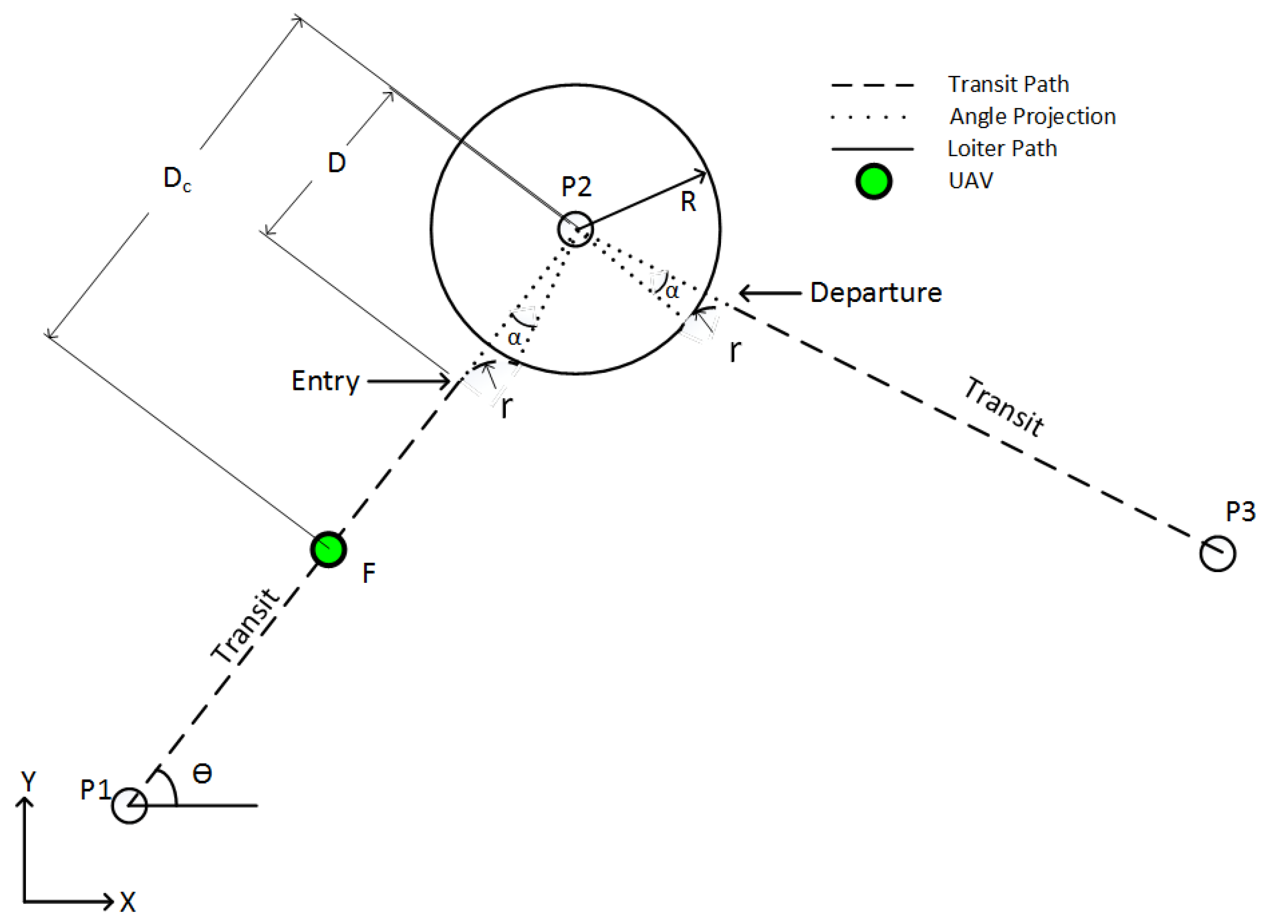
The LDLPP algorithm started by calculating a bearing angle between a start point and the first POI. The transit maneuver was then initiated by generating straight line segments in the direction of the bearing angle until the UAV reached a predetermined distance from the POI. When the UAV reached distance from the POI, the straight line segment transit maneuver was terminated and then the curved entry maneuver was initiated. The curved entry maneuver consisted of turning the UAV at a constant turn rate until the vehicle was directly over the first AOI perimeter. When the UAV was on the AOI’s perimeter, the curved entry maneuver was terminated and the loitering maneuver was initiated by turning the UAV in a CCW direction. The loitering maneuver continued until two conditions were met. The first condition required that the UAV had circled the AOI completely at least once. The second condition compared the angle between the craft, the current POI, and the next POI to a predetermined entry/departure angle . When the UAV had completed at least one turn and was at degrees with respect to the current and subsequent POIs, the loiter maneuver was terminated and the CW circular exit turn was initiated. The curved exit turn was performed at the same turn rate as the entry turn. Once the UAV tangentially intercepted the line connecting the current and subsequent POIs, the exit turn was terminated and the LDLPP was restarted, commanding the UAV to transit to the next POI. The LDLPP path for a transit, entry, loiter, exit, and transit set of maneuvers described is shown in Figure 10 where the transit path is denoted with a dashed line, angle projections are denoted with a dotted line, the loiter path is denoted by a solid line and the vehicle position is marked by a green circle.
In reference to the POI geometry presented in Figure 10, the three POI positions are expressed in the same notation presented in Equation (1). The position vector of the UAV is expressed similarly, but in this case it takes the form presented in Equation (13):
where is the X coordinate of UAV and is the Y coordinate of UAV. Note that the position of a UAV, as represented in Figure 10, is at that of an arbitrary time during the simulation. The bearing angle, , between POI 1 and POI 2, was then calculated through Equation 8. With the positions of , , , F, and the bearing angle assigned, the straight line transit maneuver was generated with a slope of . The entry/departure angle, , provided the angle at which the UAV flying along the turn radius, r, would lie tangent to the AOI radius, R, measured about the next POI. The calculation for which is shown in Equation (14):
where R is the radius of the AOI and r is the turn radius of vehicle. An example of the associated angle projection is shown in Figure 10. The closing distance was calculated from the current position of the UAV using Equations (2)–(4), while the curved entry distance, , was calculated as a function of the vehicle turn radius, r, AOI radius, R and entry/departure angle, . The straight line transit maneuver was executed until the closing distance of the UAV, , was equal to the entry distance, , which is calculated in Equation (15):
where R is the radius of the AOI, r is the turn radius of vehicle, and is the entry/departure angle.
Once the closing distance, , was equal to the entry distance, , the straight line transit maneuver was terminated and a CW turn of constant radius, r, was initiated. The change in heading throughout the entry turn, , was tracked in order to determine when the entry turn could be considered complete. Entry turn heading change was calculated by taking the absolute difference of the current heading and the heading at the start of the entry turn, , as shown in Equation (16):
where is the current heading of UAV and is the heading of UAV at the start of entry turn. Once the change in heading, , became equal to the entry/departure angle , the CW entry turn was terminated and the position of the aircraft was said to be on the perimeter of the AOI.
The loiter maneuver was then initiated in a CCW direction with a turning radius equivalent to the radius of the AOI, R, and was executed until two conditions were satisfied. The first condition required that a 360 turn around the perimeter of the AOI be completed, while the second condition required that the angle between the UAV and POI 3 with respect to POI 2 be equal to .
The closing angle, , followed a similar concept to that of in which the angle between the UAV and the departure angle with respect to the current POI was tracked around the loiter to determine the instant at which the UAV could exit the loiter in the direction of the next POI. The closing angle between POI 2 and POI 3, , was calculated by taking the inverse tangent of a quotient containing the absolute value of a determinant and a dot product, shown in Equation (17):
where is the UAV position vector, is the POI 2 position vector, and is the POI 3 position vector. The loitering maneuver was terminated and the exit turn was initiated. Figure 11 presents a scenario wherein the UAV, denoted as F, is assumed to have completed a 360 trip around the AOI and approaches the departure angle from a CCW direction that will align the UAV with POI 3.
Similar to the entry turn, the heading of the UAV throughout the exit turn was tracked using Equation (16) until the change in the heading angle was equal to the entry/departure angle . Once equal, the exit turn was terminated and the algorithm returned to the first step, generating straight line segments to the next POI.
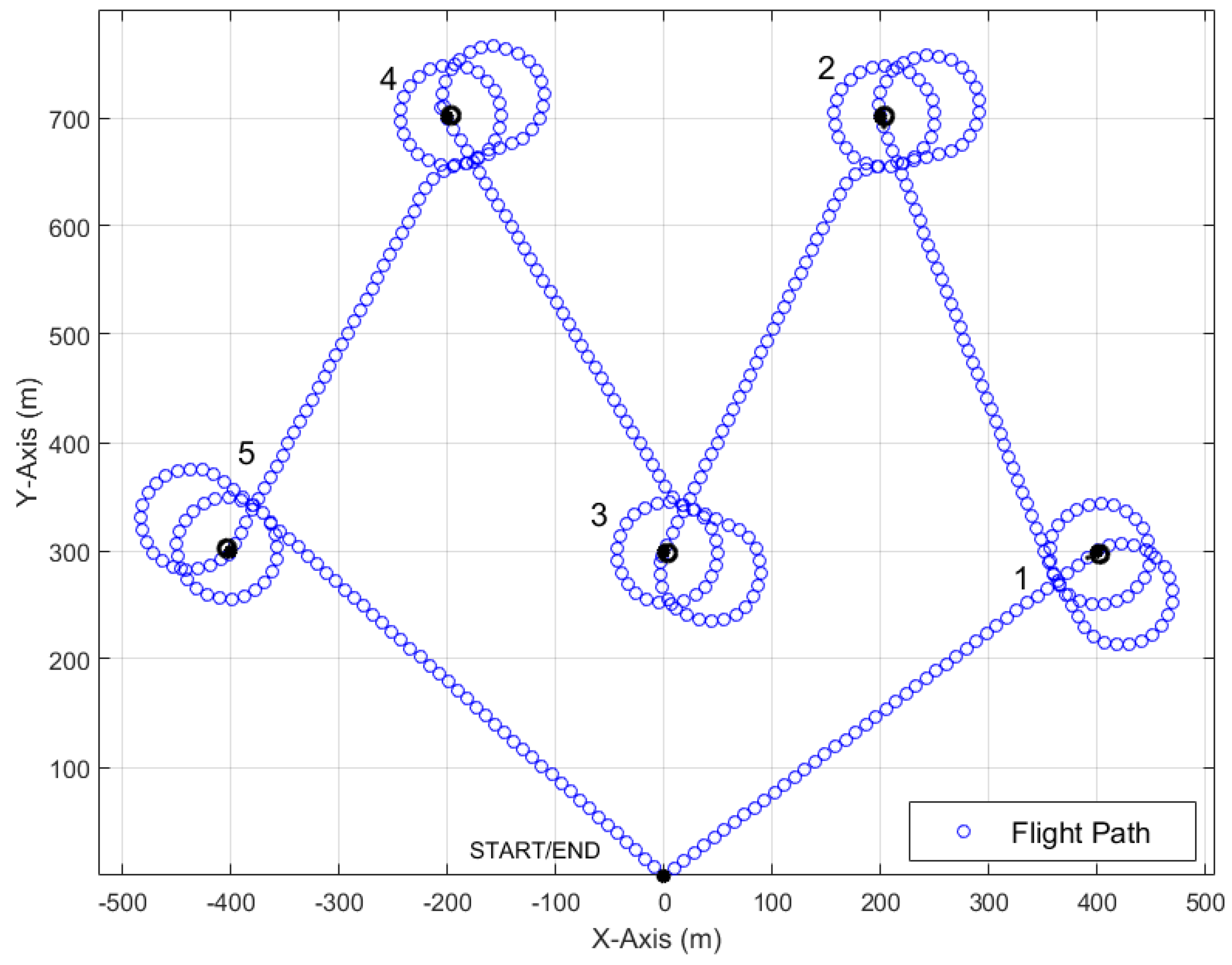
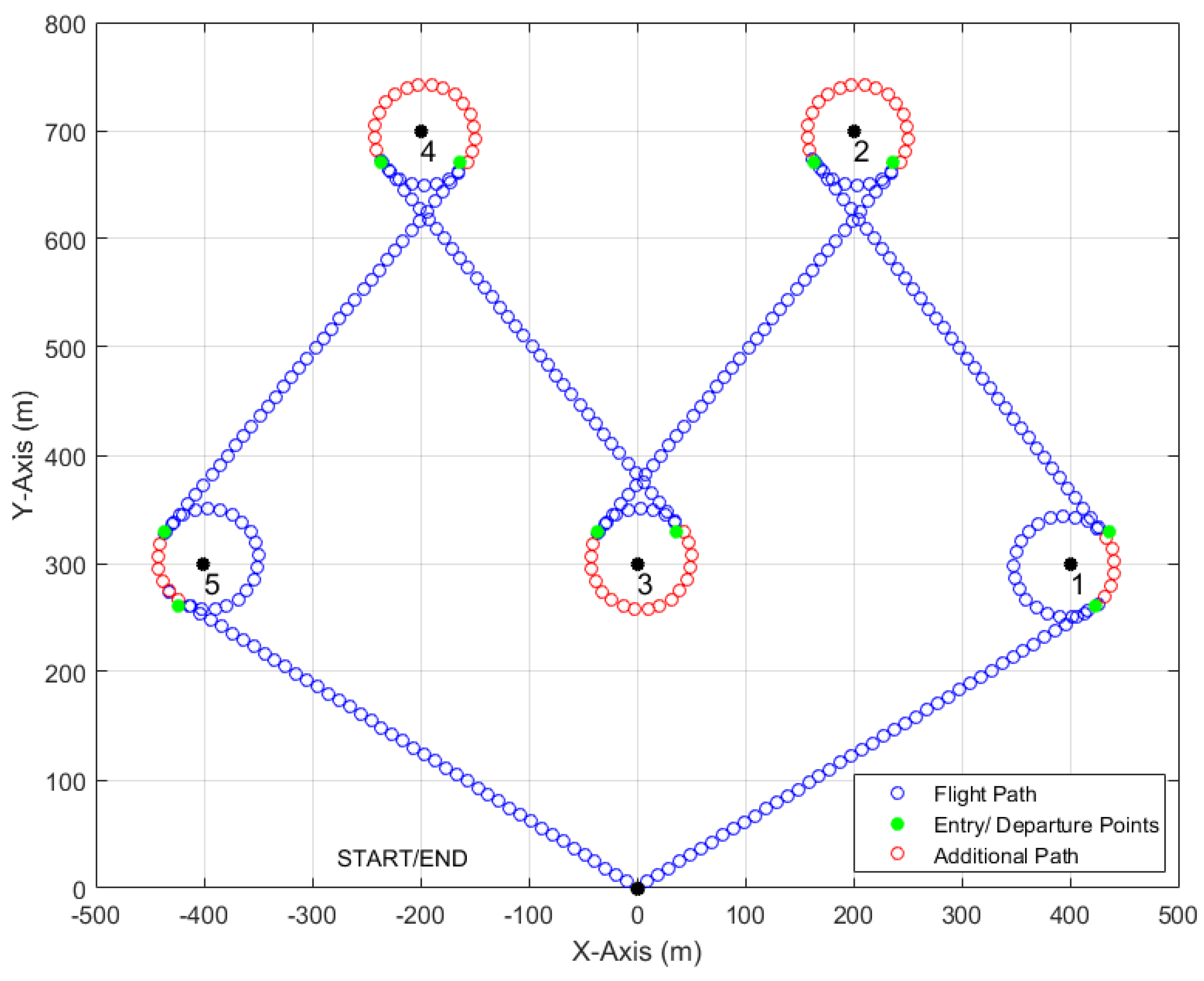
If the next waypoint was a POI, the UAV would begin the transit, entry, loiter, and exit loop over again. If the next waypoint was the endpoint of the simulation, the UAV would simply transit to the endpoint using straight line transit segments. Once the UAV reached the endpoint, the simulation terminated. A five POI simulation utilizing the LDLPP method is presented in Figure 12, where the UAV starts at (0,0) and surveys five POIs in numerical order before returning to the START/END point.
4. Path Planning Simulations
4.1. Simulation Parameters
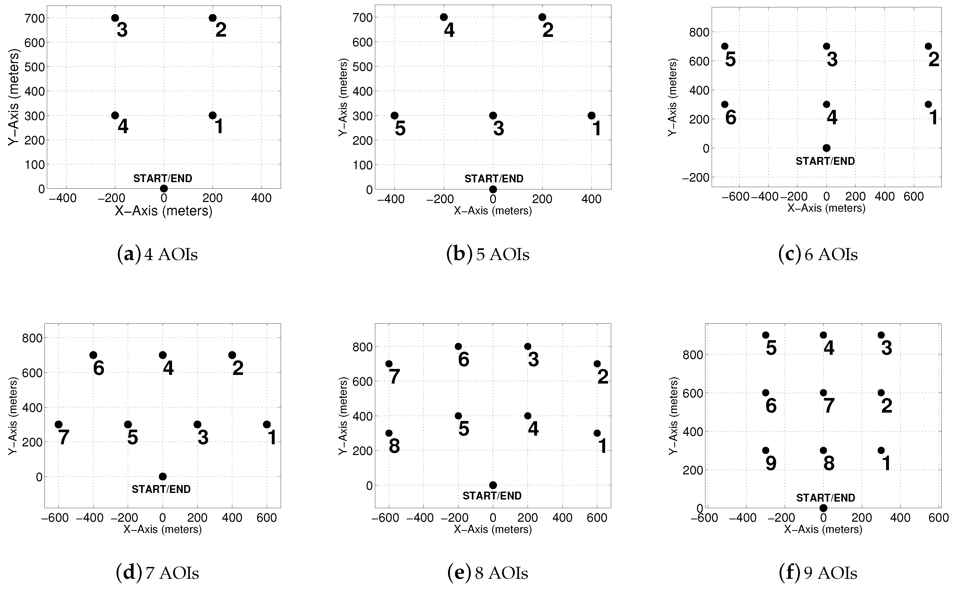
Six simulation scenarios were programmed into MATLAB, which are shown in Figure 13. The scenarios consist of four to nine POIs in various configurations in order to determine how well the algorithms perform under various ranges of operation. The START and END waypoints for each scenario were located at (0,0) and all POIs were restricted to an 800 × 800 m area. The radius of the AOI was set equal to the minimum turning radius of the vehicle and held constant for all simulations. A waypoint was generated for each one second time step. It was assumed that the UAV had equivalent properties to Raven RQ-11B: turning radius of 46 m, cruising speed of 12 m/s, and a turn-rate of 14 /s
A requirement was established in which 75% of the AOI must be within the cameras’ FOV in order to be considered as coverage. Quantifying coverage in this way could allow for post-processing stitching of the surveillance images to assemble a complete image of the AOI. Coverage time was then defined as the sum of time steps where the camera’s FOV experienced sensor coverage of 75% or more of the AOI. Lastly, for each simulation, the UAV was required to complete at least one turn around the AOI before transiting to the next AOI.
4.2. Simulation Results
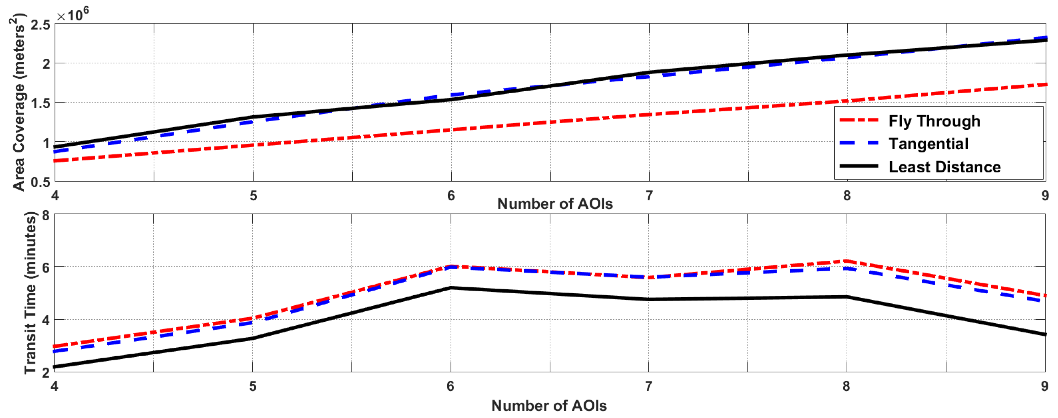
The flight time and area coverage for the three loitering techniques are summarized in Table 1. It can be expected that with an increasing number of AOIs, both flight time and AOI coverage will increase. This trend held true for all AOI coverage measurements; however, for the nine AOI scenarios, there is a slight drop in flight time for all three methods. The decrease in flight time from eight to nine AOIs is due to the arrangement and order.
In order to further compare the three loitering methods, it is beneficial to look at not only the total flight time and area coverage, but the time spent in transit between AOIs. Using Table 1 in tandem with Figure 14, a comparison can be made between the three loitering methods. From Table 1, it is shown that the LDLPP method consistently achieves the lowest flight times of the three methods examined. This may primarily be attributed to the decrease in transit time produced by optimizing the flight path between AOIs, shown in the bottom graphic of Figure 14. In addition, the top graphic of Figure 14 demonstrates that while the transit time is significantly decreased for the LDLPP method, it still achieves an average AOI coverage that is higher than that of the TLPP method. From the results presented, it can be said that the LDLPP method maximized the AOI coverage while minimizing flight times. Maximum coverage and minimal flight times were achieved by eliminating unnecessary turns outside of the AOI as well as reducing transit distance.
5. Conclusions
Traditional Fly Through loitering for an aircraft was investigated to determine if a more efficient path could be undertaken to avoid unnecessary and extra turns to enter a loiter. Modeling of flight was achieved using pose-based Dubins aircraft algorithms. Three algorithms for loitering were evaluated based on overall flight time and AOI coverage. The Fly Through loitering method required that the UAV fly directly over the center of an AOI before entering into a loiter path around the AOI. Two new methods, the Tangential Loitering Path Planner method and Least Distance Loitering Path Planner method, were developed to include intelligent entrance and exits around an AOI loiter path. The Fly Though Loitering method typically resulted in unwanted extra turns due to the loiter entry through the center of an AOI. The TLPP and LDLPP methods allowed the aircraft to directly enter a loiter from a strategic position located outside the AOI, thus eliminating unnecessary turning. It was concluded that both the TLPP and LDLPP methods have superior coverage for a given number of AOIs. It was also demonstrated that that the LDLPP method had the shortest transit time for the simulations ran. The implications of a lower transit time translate into more time available for AOI coverage and reduced overall flight times.
Acknowledgments
The authors would like to thank Jonathan Rojas, a recent MS graduate in Mechanical Engineering from West Virginia University (Morgantown, WV, USA), and Brian H. Berthold, an undergraduate Mechanical Engineering student at Ohio University (Athens, OH, USA), for assistance with the path planning algorithms.
Author Contributions
Jay P. Wilhelm defined and presented the current loitering methods and described the improved LLDP to the Graduate Researchers. Garrett S. Clem derived and programmed the LLDP method in MATLAB and analyzed the results for the six scenarios presented. Gina M. Eberhart assisted in programming and provided substantial edits to the final paper.
Conflicts of Interest
The authors declare no conflict of interest.
Abbreviations
The following abbreviations are used in this manuscript:
| AOI | Area of Interest |
| CCW | Counterclockwise |
| CW | Clockwise |
| FOV | Field of View |
| ISR | Intelligence, Surveillance and Reconnaissance |
| LDLPP | Least Distance Loitering Path Planner |
| LOS | Line of Sight |
| POI | Point of Interest |
| TLPP | Tangential Loitering Path Planner |
| UAV | Unmanned Aerial Vehicle |
References
- Colomina, I.; Molina, P. Unmanned aerial systems for photogrammetry and remote sensing: A review. ISPRS J. Photogramm. Remote Sens. 2014, 92, 79–97. [Google Scholar] [CrossRef]
- Fudge, M.; Stagliano, T.; Tsiao, S. Non-Traditional Flight Safety Systems & Integrated Vehicle Health Management Systems; Report for the Federal Aviation Administration; ITT Ind.: Alexandria, VA, USA, 2003. [Google Scholar]
- Dempsey, M.E.; Rasmussen, S. Eyes of the Army–US Army Roadmap for Unmanned Aircraft Systems 2010–2035; US Army UAS Center of Excellence: Fort Rucker, AL, USA, 2010; Volume 9. [Google Scholar]
- Air-Force-Special-Operations-Command. RQ-11B Raven System 2009. Available online: http://www.avinc.com/downloads/USA_Raven_FactSheet.pdf (accessed on 1 September 2016).
- Van Bourgondien, J. Analysis of the Sustainment Organization and Process for the Marine Corps’ RQ-11B Raven Small Unmanned Aircraft System (SUAS); Technical Report; DTIC Document: Fort Belvoir, VA, USA, 2012. [Google Scholar]
- Alighanbari, M.; Kuwata, Y.; How, J.P. Coordination and control of multiple UAVs with timing constraints and loitering. In Proceedings of the 2003 IEEE American Control Conference, Denver, CO, USA, 4–6 June 2003; Volume 6, pp. 5311–5316. [Google Scholar]
- Rathinam, S.; Almeida, P.; Kim, Z.; Jackson, S.; Tinka, A.; Grossman, W.; Sengupta, R. Autonomous searching and tracking of a river using an UAV. In Proceedings of the 2007 IEEE American Control Conference, New York, NY, USA, 11–13 June 2007; pp. 359–364. [Google Scholar]
- Sujit, P.; Saripalli, S.; Sousa, J. An evaluation of UAV path following algorithms. In Proceedings of the 2013 IEEE European Control Conference (ECC), Zurich, Switzerland, 17–19 July 2013; pp. 3332–3337. [Google Scholar]
- Wu, H.; Sun, D.; Zhou, Z. Model identification of a micro air vehicle in loitering flight based on attitude performance evaluation. IEEE Trans. Robot. 2004, 20, 702–712. [Google Scholar] [CrossRef]
- 3D-Robotics. The Pixhawk Autpilot System. 2015. Available online: http://store.3drobotics.com/products/3dr-pixhawk (accessed on 1 September 2016).
- Wilhelm, J.; Rojas, J. Development of an Area of Interest Extended Coverage Loitering Path Planner. In Proceedings of the AIAA Infotech@Aerospace, AIAA SciTech Forum, San Diego, CA, USA, 4–8 January 2016. [Google Scholar]
- LaValle, S.M. Planning Algorithms; Cambridge University Press: New York, NY, USA, 2006. [Google Scholar]
- Riviere, S.; Schmitt, D. Two-dimensional line space Voronoi Diagram. Voronoi Diagrams in Science and Engineering. In Proceedings of the 2007 4th International Symposium (ISVD ’07), Pontypridd, UK, 9–11 July 2007; pp. 168–175. [Google Scholar]
- Araújo, J.F.; Sujit, P.B.; Sousa, J.B. Multiple UAV Area Decomposition and Coverage. In Proceedings of the 2013 IEEE Symposium on Computational Intelligence for Security and Defense Applications (CISDA), Athens, Greece, 16–19 April 2013; pp. 30–37. [Google Scholar]
- Dubins, L.E. On Curves of Minimal Length with a Constraint on Average Curvature, and with Prescribed Initial and Terminal Positions and Tangents. Am. J. Math. 1957, 79, 497–516. [Google Scholar] [CrossRef]
- Grymin, D.J.; Crassidis, A.L. Simplified model development and trajectory determination for a UAV using the Dubins set. In Proceedings of the AIAA Atmospheric Flight Mechanics Conference, Chicago, IL, USA, 10–13 August 2009; p. 6050. [Google Scholar]
- Karas, O. UAV Simulation Environment for Autonomous Flight Control Algorithms. Master’s Thesis, West Virginia University, Morgantown, WV, USA, 2012. [Google Scholar]
- Wilburn, J.N. Development of an Integrated Intelligent Multi-Objective Framework for UAV Trajectory Generation. Ph.D. Thesis, West Virginia University, Morgantown, WV, USA, 2013. [Google Scholar]
- Shanmugavel, M.; Tsourdos, A.; White, B.; Żbikowski, R. Co-operative path planning of multiple UAVs using Dubins paths with clothoid arcs. Control Eng. Pract. 2010, 18, 1084–1092. [Google Scholar] [CrossRef]
- Al Nuaimi, M. Analysis and Comparison of Clothoid and Dubins Algorithms for UAV Trajectory Generation. Master’s Thesis, West Virginia University, Morgantown, WV, USA, 2014. [Google Scholar]
- Savla, K.; Bullo, F.; Frazzoli, E. The coverage problem for loitering Dubins vehicles. In Proceedings of the IEEE 2007 46th IEEE Conference on Decision and Control, New Orleans, LA, USA, 12–14 December 2007; pp. 1398–1403. [Google Scholar]
- Lugo-Cárdenas, I.; Flores, G.; Salazar, S.; Lozano, R. Dubins path generation for a fixed wing UAV. In Proceedings of the 2014 IEEE International Conference on Unmanned Aircraft Systems (ICUAS), Orlando, FL, USA, 27–30 May 2014; pp. 339–346. [Google Scholar]
Figure 1.
Fly through loiter path entry.

Figure 2.
Fly over path planner flowchart.

Figure 3.
Path segmentation.
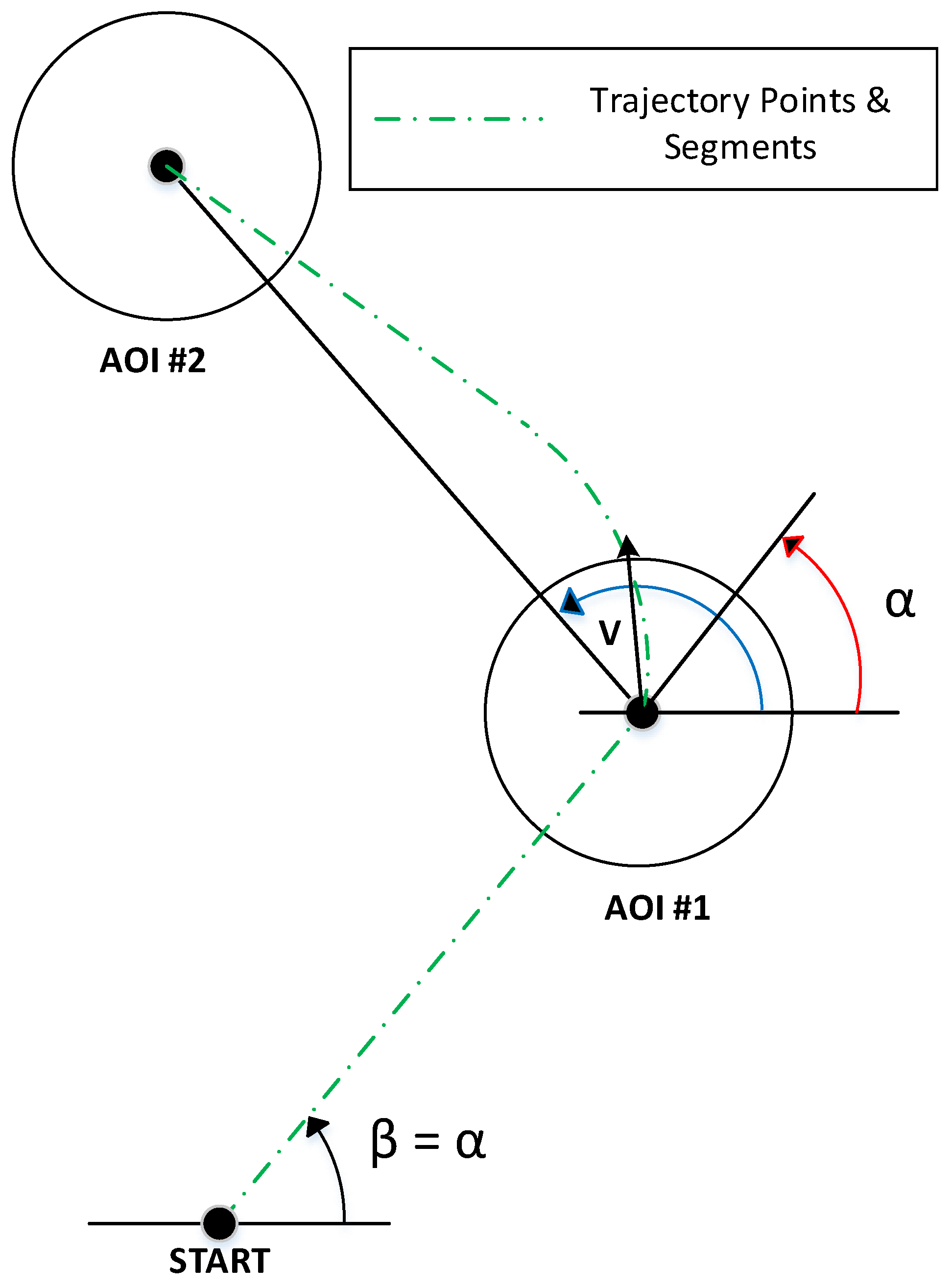
Figure 4.
Nominal (a) and 25 Rotated (b) Camera Gimbal.
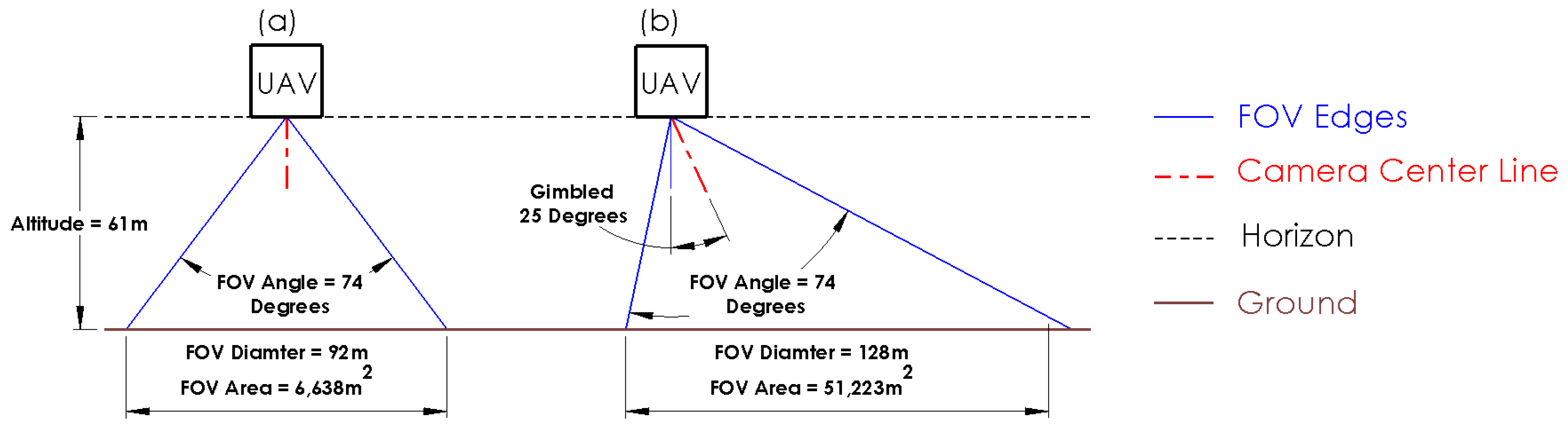
Figure 5.
Fly through loiter path entry.

Figure 6.
Fly through loiter.

Figure 7.
Tangent point circle.

Figure 8.
Inner tangents.

Figure 9.
Tangential loitering path.

Figure 10.
Least distance smart loiter transit, entry, loiter, departure path.

Figure 11.
Angle between vehicle and POIs.
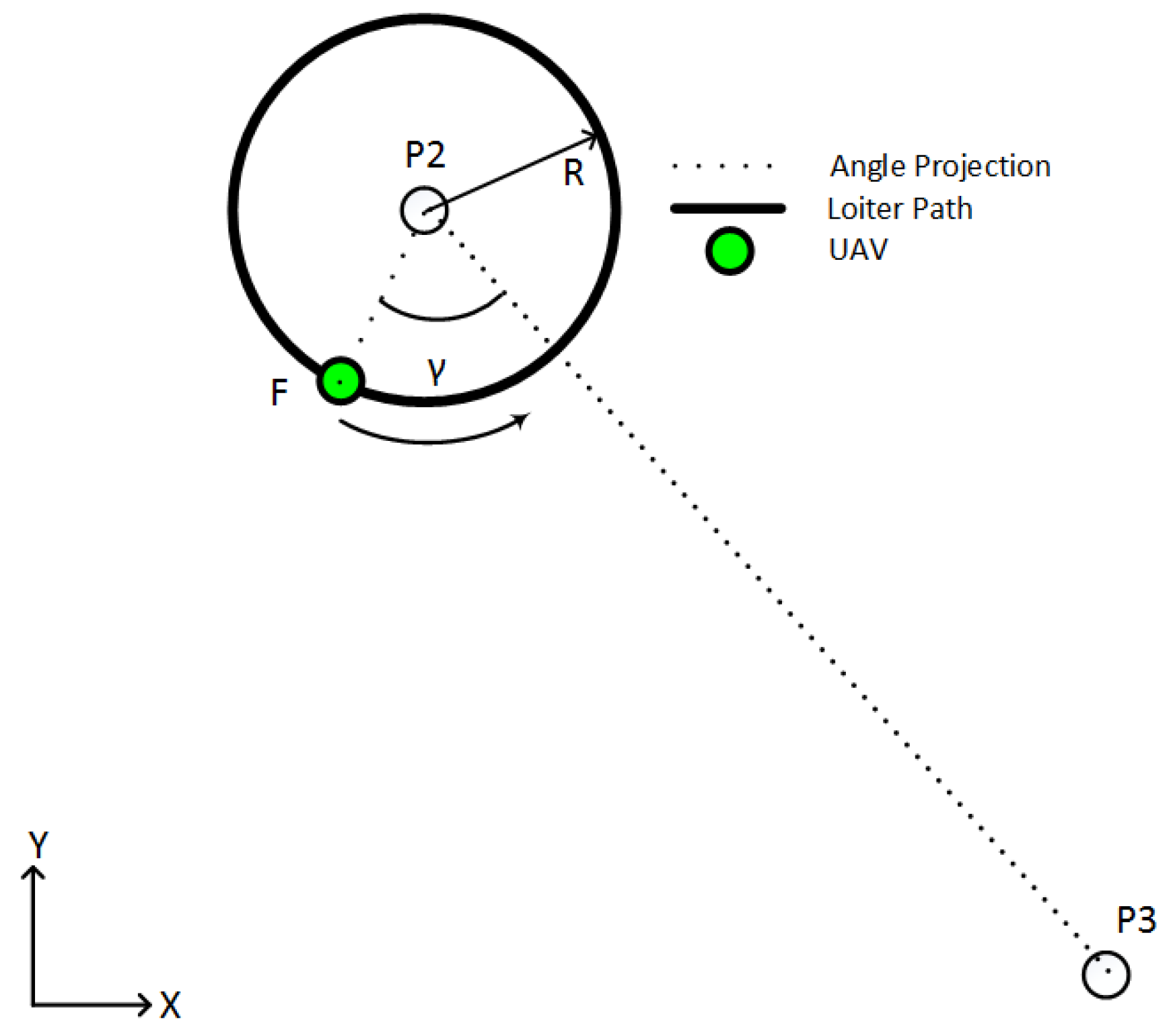
Figure 12.
Least distance smart loitering path for five POIs.
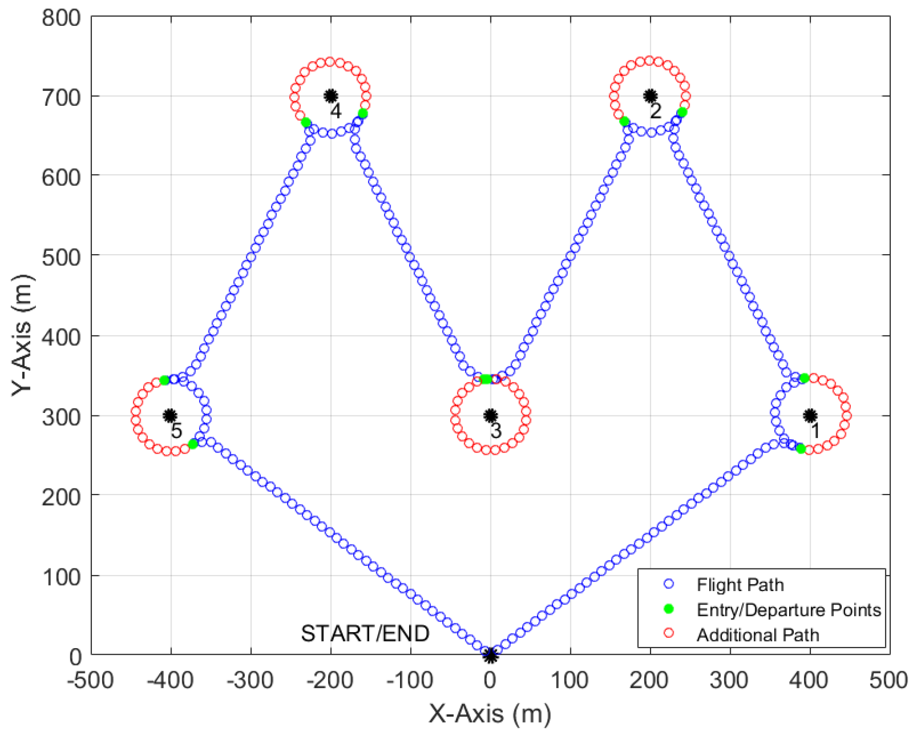
Figure 13.
Simulation scenarios.

Figure 14.
Comparison of fly through, tangential smart loiter, and least distance loitering methods.
Figure 14.
Comparison of fly through, tangential smart loiter, and least distance loitering methods.

Table 1.
Simulation results.
| Method | Parameters | 4 AOIs | 5 AOIs | 6 AOIs | 7 AOIs | 8 AOIs | 9AOIs |
|---|---|---|---|---|---|---|---|
| Fly Through | Flight Time (min) | 6.03 | 7.90 | 10.82 | 11.18 | 12.37 | 12.01 |
| AOI Coverage (m) | 756,180 | 955,796 | 1,150,033 | 1,344,934 | 1,517,409 | 1,727,275 | |
| TLPP | Flight Time (min) | 4.89 | 7.07 | 9.99 | 10.28 | 11.04 | 10.32 |
| AOI Coverage (m) | 873,713 | 1,253,878 | 1,594,026 | 1,827,461 | 2,067,565 | 2,321,009 | |
| LDLPP | Flight Time (min) | 4.51 | 6.55 | 9.03 | 9.45 | 10.07 | 9.10 |
| AOI Coverage (m) | 933,739 | 1,313,904 | 1,534,000 | 1,880,817 | 2,100,913 | 2,287,660 |
© 2017 by the authors. Licensee MDPI, Basel, Switzerland. This article is an open access article distributed under the terms and conditions of the Creative Commons Attribution (CC BY) license (http://creativecommons.org/licenses/by/4.0/).
Share and Cite
MDPI and ACS Style
Wilhelm, J.P.; Clem, G.S.; Eberhart, G.M. Direct Entry Minimal Path UAV Loitering Path Planning. Aerospace 2017, 4, 23. https://doi.org/10.3390/aerospace4020023
AMA Style
Wilhelm JP, Clem GS, Eberhart GM. Direct Entry Minimal Path UAV Loitering Path Planning. Aerospace. 2017; 4(2):23. https://doi.org/10.3390/aerospace4020023
Chicago/Turabian StyleWilhelm, Jay P., Garrett S. Clem, and Gina M. Eberhart. 2017. "Direct Entry Minimal Path UAV Loitering Path Planning" Aerospace 4, no. 2: 23. https://doi.org/10.3390/aerospace4020023
Note that from the first issue of 2016, this journal uses article numbers instead of page numbers. See further details here.