
Multi-Mode Electric Actuator Dynamic Modelling for Missile Fin Control


Aeromechanical Systems Group, Centre for Defence Engineering, Cranfield University, Defence Academy of the United Kingdom, Shrivenham, Swindon SN6 8LA, UK
*
Author to whom correspondence should be addressed.
Aerospace 2017, 4(2), 30; https://doi.org/10.3390/aerospace4020030
Submission received: 31 March 2017
/
Revised: 7 June 2017
/
Accepted: 8 June 2017
/
Published: 14 June 2017
Abstract
:Linear first/second order fin direct current (DC) actuator model approximations for missile applications are currently limited to angular position and angular velocity state variables. Furthermore, existing literature with detailed DC motor models is decoupled from the application of interest: tail controller missile lateral acceleration (LATAX) performance. This paper aims to integrate a generic DC fin actuator model with dual-mode feedforward and feedback control for tail-controlled missiles in conjunction with the autopilot system design. Moreover, the characteristics of the actuator torque information in relation to the aerodynamic fin loading for given missile trim velocities are also provided. The novelty of this paper is the integration of the missile LATAX autopilot states and actuator states including the motor torque, position and angular velocity. The advantage of such an approach is the parametric analysis and suitability of the fin actuator in relation to the missile lateral acceleration dynamic behaviour.
1. Introduction
Previous research has mainly focused on the system performance by comparing the commanded and the actual deflection of the missile fin (angular position). There is a simplified assumption that the actuator supplies instantly the required load torque to the fin to hold it in its position under the given aerodynamic flow conditions. However, in this paper, the missile fin is driven from a direct-drive actuator without a gearbox. Hence, the holding torque at different fin angular positions must be supplied from the actuator alone. Moreover, the load torque cannot be provided instantaneously from the actuator and the current is modelled to allow a better understanding of the missile lateral acceleration (LATAX) characteristics in relation to the fin actuator electrical characteristics. Normally, missiles consist of three fundamental operational blocks in relation to Control and Guidance (see Figure 1): the fin actuators (Level 1); the airframe autopilot (Level 2); and the airframe guidance (Level 3). This paper aims to integrate a direct-drive actuator with the missile fin dual feedforward/feedback model and relate this to the missile airframe state variables. The missile is tail-fin controlled and the airframe motion considered is LATAX. The aim is to identify the key relationships that will allow the observation of the direct current (DC) motor torque for the aerodynamically-loaded fin in relation to the airframe lateral acceleration thus resulting in useful correlations between Levels 1 and 2.
The missile autopilot normally needs to be fast and responsive since very short timings are involved during the target engagement process. Slower responses can lead to a target miss, especially if the target has a high-g manoeuvring capability.
Hwang et al. [1] have used an actuator with second-order non-linear dynamics for studying the adaptive sliding mode control of actuators for a missile. This study emphasises the angular response and the track errors of the actuator. Liu et al. [2] have used a second-order electromechanical actuator servo system to understand the tracking precision and suppression of chatter at control input using a global sliding mode controller for a missile. Tsourdos et al. [3] have modelled an actuator as second order for studying the autopilot response for highly nonlinear missile aerodynamics and unknown parameters. Buschek [4] has modelled the actuator of a roll-position autopilot for the IRIS-T air-to-air missile as second-order with uncertainty on natural frequency to introduce changing actuator performance under various loading conditions (IRIS-T: A German-led international missile programme. The name derives from Infra-Red Imaging System Tail/Thrust Vector-Controlled.). Kim et al. [5] have modelled the actuator with first-order dynamics for a pitch controller of a bank-to-turn (BTT) missile. Devaud et al. [6] in their study of control strategies for a high-angle-of-attack missile autopilot have modelled an actuator with first-order dynamics and analysed the position and rate output sensitivity with different operating points. Menon et al. [7] studied the actuator blending logic that optimally selects a mix of actuators (aerodynamic tail fins or thrusters) at various flight conditions of a ship defence missile. Tahk et al. [8] modelled an actuator with second-order dynamics suitable for both BTT and skid-to-turn (STT) missiles, and analysed the autopilot performance for both initial condition and missile position operation modes. Hirokawa et al. [9] have studied an application blending aero-fin and reaction-jet effectors in a missile autopilot to improve the guidance performance against highly manoeuvrable targets with an actuator of first-order dynamics.
Shtessel et al. [10] in their study of integrated higher-order sliding mode guidance and autopilot for dual-control missiles (combination of aerodynamic lift, sustained thrust and centre-of-gravity divert thrusters) have considered a second-order autopilot model, which indicates the actuator has first-order dynamics, and analysed the response of the missile in angular positions only. Mehrabian et al. [11] have modelled an actuator with second-order dynamics for a tail-controlled missile to study a STT missile autopilot design using adaptive control methodology based on eigen-structure assignment wherein the response of the missile is assessed by tail fin deflection and pitching rate. Reichert [12] has designed an autopilot for a tail-fin controlled missile using dynamic scheduling in which the actuator is modelled with second-order dynamics and has analysed the system performance for a series of commanded manoeuvres at varying speeds in terms of missile angle of attack only. Talole et al. [13] in their roll autopilot design based on an extended state observer technique have modelled an actuator with second-order dynamics for the position servo and analysed the system performance based on roll angle only. Chwa et al. [14] in their study of compensation of the actuator dynamics in a nonlinear missile control have modelled a second-order actuator and proposed a compensation methodology to avoid the destabilisation of the control loops due to the actuator. The system performance with the compensator is analysed only for the fin deflection angle. Menon et al. [15] have discussed the design of a blended actuator with fin actuator and reaction-jet using adaptive techniques. The fin actuator is modelled with second-order dynamics. The overall system performance was analysed with respect to the commanded position and missile actual position using the states of a six-degree-of-freedom model.
In this paper, an actuator architecture is proposed and analysed that ensures the delivery of the required fin torque under different aerodynamic flow conditions. This proposed architecture needs the details of the load torque required by the missile fin with respect to the angle of attack at the given flight conditions. The actuator was also checked with the dual-feedback LATAX autopilot. Previous work in the literature has represented the fin servo system without modelling the fin aerodynamic load torque and actuator torque. In this paper, the work differs because the fin torque is modelled and related to the system autopilot design. Thus, offering parametric correlations between missile airframe LATAX performance and fin actuator performance with visibility of the torque and hence electrical current requirements. Consequently, designers for given LATAX airframe trajectories can predict, based on the modelling developed in this paper, the power and energy requirements of their power supply.
The paper is structured as follows: Section 2 presents the proposed actuator model including the feedforward and feedback architecture. Section 3 presents the autopilot design and the integration to the feedforward/feedback actuator model. Section 4 presents the simulation results for both the actuator model and the autopilot systems. Section 5 presents the conclusions.
2. Actuator Model (Level 1)
A direct-drive electric actuator (DDEA) is used for the missile fin actuation. The general schematic of the actuator, fin and the missile are shown in Figure 2. A DDEA normally has a negligible holding torque and as a result the actuator normally needs to be actively powered to sustain the fin at a desired position. Due to the range of flight conditions, the load torque as experienced by the fin will vary and requires continuous control action to maintain position. The DDEA is supplied with the required electric power (Pin) from the missile on-board power system. It is assumed that the electrical supply provides a stabilised power irrespective of the actuator load demands. Figure 2 shows that the motor load due to the fin and aerodynamic forces are related to the missile speed and fin geometry. The aerodynamic forces are a function of the missile’s flight conditions and, more generally, the missile and fin geometry. Availability of the torque variable, and therefore the current, allows designers to investigate how the missile airframe manoeuvrability influences the torque demand for a range of test conditions as shown in Section 4. This results in improving the understanding of the fin actuator characteristics in relation to the airframe LATAX motion. This is significant, because it allows correlations of electrical fin-related variables and airframe motion variables. Figure 2 shows the DDEA, input power per actuator, the aerodynamic airflow, and fin motion variables.
The block diagram indicating the missile guidance architecture utilised in this paper is shown in Figure 1. In the proposed system, the actuator has two parts: System A and System B. System A consists of the DDEA for driving the missile fin, which also considers the initial conditions of the missile fin position. It is a position servo system that can be used both for positioning (set point inputs) or missile stabilisation functions. The actuator model is a conventional servo system with proportional and derivative control. The load torque is algebraically estimated based on the missile aerodynamic flight conditions for the given fin geometry utilising a gain scheduler feedforward based control strategy.
The autopilot architecture applied is shown in Figure 3. The missile LATAX autopilot receives demands from the guidance to engage the target. The autopilot consists of the actuator/fin and the missile airframe.
System A (Figure 3) is shown in more detail in Figure 4 in relation to the aerodynamic fin load (Figure 5). Figure 4 shows the control architecture for the two key operational modes: stabilisation mode and position mode. For the stabilisation mode, when the demand is zero it is important for the control system to reject any fin load disturbances (gusts for example). For the position mode the control system is required to maintain zero steady-state error and quick performance (transient). For both modes within this proposed architecture the DC motor actuator is required to supply the entire torque since the topology is direct drive rather than a geared solution which provides a good amount of holding torque.
System B consists of load torque details required by the missile fin for the given aerodynamic flow conditions. Here, the missile flight speed is considered as Mach 2.0 and the associated load torque characteristics against the fin angle of attack between −15° and +15° is assumed to be linear with a slope of 0.52 Nm/°, as shown in Figure 5. The characteristic shown in Figure 5 is fixed for a given missile flight condition and geometry.
The missile can operate at different times in either a set point fin deflection mode, or an initial condition (IC) mode. Depending upon which mode the missile is operating in, the load torque is utilised from the error signal (θe) or from the demanded position angle (θd) respectively. In both cases the load torque characteristic against fin angle of attack is the same. The block diagram of System B is shown in Figure 6.
Based on [16], the steady-state characteristics of the actuator with a back EMF are given from Equation (1) relating the motor angular velocity and electrical current for given input voltage Va,
where is the angular velocity of the actuator shaft linked to the fin in [rad/s]. is the actuator electrical current flowing through the windings. The electrical current is proportional to the torque developed by the motor (Equation (3)). Normally, for a constant excitation voltage and constant load torque, the angular velocity will start reducing as the load torque increases. With the inclusion of dynamics, the equation for the actuator is given by
where represents the actuator winding inductance in [H]. Therefore, Equation (2) allows the examination of the actuator dynamics while Equation (1) is limited to steady-state values. is the actuator winding resistance in [Ω] representing the Ohmic power losses within the actuator. Ideally, it is desirable to have low resistance so that when the motor is operating at high load values (i.e., the current is also high) then the Ohmic or copper losses can remain as low as possible. In practice, external conditions such as airflow and the actuator autopilot steering demands can affect the actuator load requirements. The torque exerted by the motor due to the current i(t) is given by
Feedforward Term
The feedforward control approach is well established and used in [17,18,19,20] with different combinations of feedback methods. Based on [16], the load torque can be added to the motor-generated torque. For this particular application, the missile fin properties are kept constant however the aerodynamic forces experienced by the fin vary based on the fin angle, hence the load torque is variable. The total torque exerted by the actuator to drive the missile fin is given, therefore, from Equation (4a) as
Function is defined from Equation (4b) as
Thus combining Equations (4a) and (4b), the total torque exerted by the actuator to drive the missile fin is given from Equation (5) as
where , for a fixed missile velocity, is the fin load torque for given fin angles provided from known aerodynamic conditions. For this model, is a linear characteristic. This is implemented in the simulation in the form of a look-up table.
If J is the actuator inertia and B is the frictional constant, the total torque exerted on the missile fin is given as
The open loop transfer function for a missile fin angle for given input voltage is as follows
where Kp is the forward proportional gain. The transfer function for both conditions (Equations (1) and (2)) as described in Equation (4c) are
3. Autopilot Design (Level 2)
Based on [17], the benefits of a feedforward control scheme can improve disturbance rejection performance. In practice, for feedforward the process model, inverse function is necessary. However, for this application the control process is divided into two separate parts: set point control mode and initial conditions (IC) mode. Hence as the fin position demanded from the autopilot system is either positive or negative but not zero then the fin is expected to use the feedforward fin information to produce, through the aerodynamic fin loading for the given flight conditions, the appropriate load torque as shown in [16]. This feedforward action enables the overall system to perform more rapidly.
As indicated in the System A block diagram (Figure 4), to have the architecture selection based on operations (stabilisation or position control), a stabilisation/control gain scheduler operator, (θd(t)) is introduced in the time domain and defined as
Here, indicates stabilisation mode of operation, whereas indicates missile fin positioning (set-point) operation. The gain scheduler is shown in Equation (10)
The actuator is controlled using the derivative as well as proportional control and the closed loop transfer function M(s) is,
The resulting transfer functions (Equations (1) and (2)) of the actuator feedback and feedforward design, from Equations (5) and (9), are given as
Autopilot
The LATAX autopilot design was used to test the fin actuator control design as part of the interactive airframe and fin dynamics systems (indicated in Figure 3). The weathercock mode characteristic equation with these aerodynamic derivatives is given as
with = 0.034877 and = 41.22. The zero in the derivative gain feedback path of the autopilot is given as
where zr = 0.0289 with an additional path gain of 105.93. The zero in the proportional gain feedback path of the autopilot is given as
where za = 14.0544 with an additional path gain of −10.52. The open loop transfer function of the LATAX autopilot is given as
With the modelling and stabilisation/control operators and accordingly for the actuator transfer function M(s) (from Equations (4), (9), (11) and (12)), the open loop transfer functions of the LATAX autopilot are
The closed loop transfer function of the LATAX autopilot of the tail controlled missile with the proposed actuator is given as
where kr and kα are the derivative and proportional gains of the autopilot respectively. With the modelling and (θd = 0) stabilisation/(θd ≠ 0) control operators and accordingly for the actuator transfer function M(s) (from Equations (4), (9) and (12)), the closed loop transfer functions of the LATAX autopilot are
The autopilot properties based on Equation (20) and the fin actuator properties (feedforward/feedback compensated) based on Equation (12) are based on Equation (21).
where Q is given from
Figure 7 shows the system parameterisation in more detail and the parametric system complexity. The overall system transfer function (Equations (21) and (22)) allows investigation of how the airframe LATAX is affected in relation to the missile model parameters (including airframe and actuators and fin loading effect). The fin actuator parameters; the airframe aerodynamic parameters, which are then converted to system poles and zeros; and the feedback actuator (fin) conditional gain scheduler, together with the fin loading feedforward input and the airframe autopilot gains, all contribute towards a systematic understanding in relation to the actuator capability to perform fast enough for the airframe to respond rapidly. This is of critical importance for this application. Furthermore, the missile airframe LATAX dynamic response is related, as shown earlier in the analysis, to the actuator electrical demands, i.e., voltage and electrical current, which enables the designers to parametrically evaluate different electrical actuators for the same missile airframe.
Equation (21), together with Q given from Equation (22), relates the DC actuator direct drive electromechanical parameters and the missile airframe parameter sets together with the availability of the load torque . This approach offers the potential to run extensive simulations for many LATAX scenarios and observe the airframe performance alongside the fin actuator performance thus providing useful understanding of the missile systems from Levels 1 and 2.
4. Simulation Results
Previous research [16,17] has demonstrated the effectiveness of feedforward control design. This paper aims to demonstrate the effectiveness of numerical simulation for missile actuator systems in relation to the autopilot control design. This is of interest since it reduces the resource and expense of flying real missiles. The following results are divided into two scenarios for two parts of the system: the actuator, and the missile airframe. The two scenarios are designed firstly to test the transient characteristics of the systems for the two modes (systems), and secondly for the scenario of running the system for a staircase scenario which allows the testing of both performance and stabilisation. The parameters of the actuator model are given in Table 1.
The performance of the proposed load-torque-compensated actuator was assessed with two scenarios, I and II. Scenario I is a step input, which corresponds to angular demand indicating positioning operation. Scenario II is a staircase input, which corresponds to angular demands for position operation followed by a stabilisation operation further followed by a second position operation in the negative direction. The missile is flying at Mach 2.0 () and the aerodynamic derivatives are given in Table 2. The values shown are normalised based upon the flight conditions and the missile geometry. They are typical of a statically-stable tail-controlled missile.
The actuator is also tested next with a dual-feedback LATAX autopilot the details of which are discussed in Section 4. The autopilot simulations were carried out for the same scenarios. Section 4.1 will discuss the simulation results of the actuator alone and Section 4.2 will discuss the simulation results of the actuator within a LATAX autopilot.
4.1. Actuator Simulation Results
4.1.1. Step Input
The step response corresponding to a demand of 15° over a time span of 0.5 s was fed as input to assess the various performance parameters of the actuator. The simulation results are presented in Figure 8.
Figure 8a describes the static and dynamic characteristics of the actuator. It can be observed that for a step input demand of 15°, the actuator starts from 0 rpm and 0 Nm and at the end of position servo, the motor speed goes to 0 rpm and the torque settles at 7.9 Nm. This is the load torque required by the missile fin at Mach 2.0 and fin angle of 15°. It can be observed that during the servo operation, the peak torque and speed of the actuator are 11.5 Nm and 300 rpm respectively. The time constant of the actuator is 44.53 ms (see Figure 8b). Figure 8e confirms that the actuator exerts the torque of 7.9 Nm as per the missile fin load torque requirements.
4.1.2. Staircase Input
The staircase input corresponding to angular demands for position operation followed by a stabilisation operation further followed by a second position operation in the negative direction was generated with position demands for ±5° and a stabilisation demand of 0°. Each demand had a 2 s time period. The simulation results are presented in Figure 9.
Figure 9a describes the static and dynamic characteristics of the actuator. It can be observed that, for the required inputs of +5°, 0° and −5°, the actuator starts from 0 rpm and 0 Nm and at the end, the motor speed goes to 0 rpm and the torque settles at 2.6, 0 and –2.6 Nm, respectively, i.e., at the load torque required for the missile fin at Mach 2.0. It can also be observed from Figure 9d, that the positioning and stabilisation operations are successfully achieved with very low steady-state error and with the same time constant. Figure 9e confirms that the actuator exerts the required torque to hold the missile fin in its position.
4.2. Autopilot Simulation Results
The rate and acceleration gains of the dual-feedback LATAX autopilot were chosen in such a way that the rise time, percentage overshoot and the steady-state error were about 200 ms, 10% and 0.001 g, respectively. An additional forward gain (kf) was introduced in the autopilot to maintain low steady-state error. The gains that satisfy these criteria are given in Table 3.
The various scenarios were simulated with these gains and the results are given in the subsequent sections.
4.2.1. Step Input
The step response corresponding to a demand of 1 g over a time span of 5 s was fed as input to assess the various performance parameters of the autopilot built using the proposed actuator. The simulation results are presented in Figure 10.
Figure 10 indicates that the performance of the autopilot with the proposed actuator is satisfactory for the step input demand of 1 g. Figure 10c shows that the LATAX response of the autopilot with steady-state error of 0.0006 g and the rise time is 220 ms. Figure 10b shows that the missile fin angle is always within 1° through the control loop function of the autopilot and achieves the 1 g demand. Figure 10d shows that the actuator exerts the required torque of 0.5 Nm on the missile fin to maintain the autopilot at 1 g. It may be further noted that since the aerodynamic derivatives used in the autopilot correspond to a tail-fin controlled missile, the area marked as “Region A” in Figure 10b–d indicates the effect of non-minimum phase due to the presence of zeros in the dynamical airframe/actuator model. Similarly, the non-minimum phase effect occurs for higher LATAX demands as shown from the simulation, which was conducted on the autopilot for a demand of 10 g (Figure 11).
The plots in Figure 11 indicate that the performance of the autopilot with the proposed actuator even with higher LATAX demand of 10 g has a transient characteristic that is similar to the case with the lower LATAX demand. As expected from Figure 10d and Figure 11d, the steady-state torque is higher for the larger LATAX demand, since the fin actuator needs to sustain a larger aerodynamic force.
4.2.2. Staircase Input
The staircase input of LATAX demands applied to the autopilot is given in Table 4.
The simulation was run over a span of 8 s and the results of the same are presented in Figure 12.
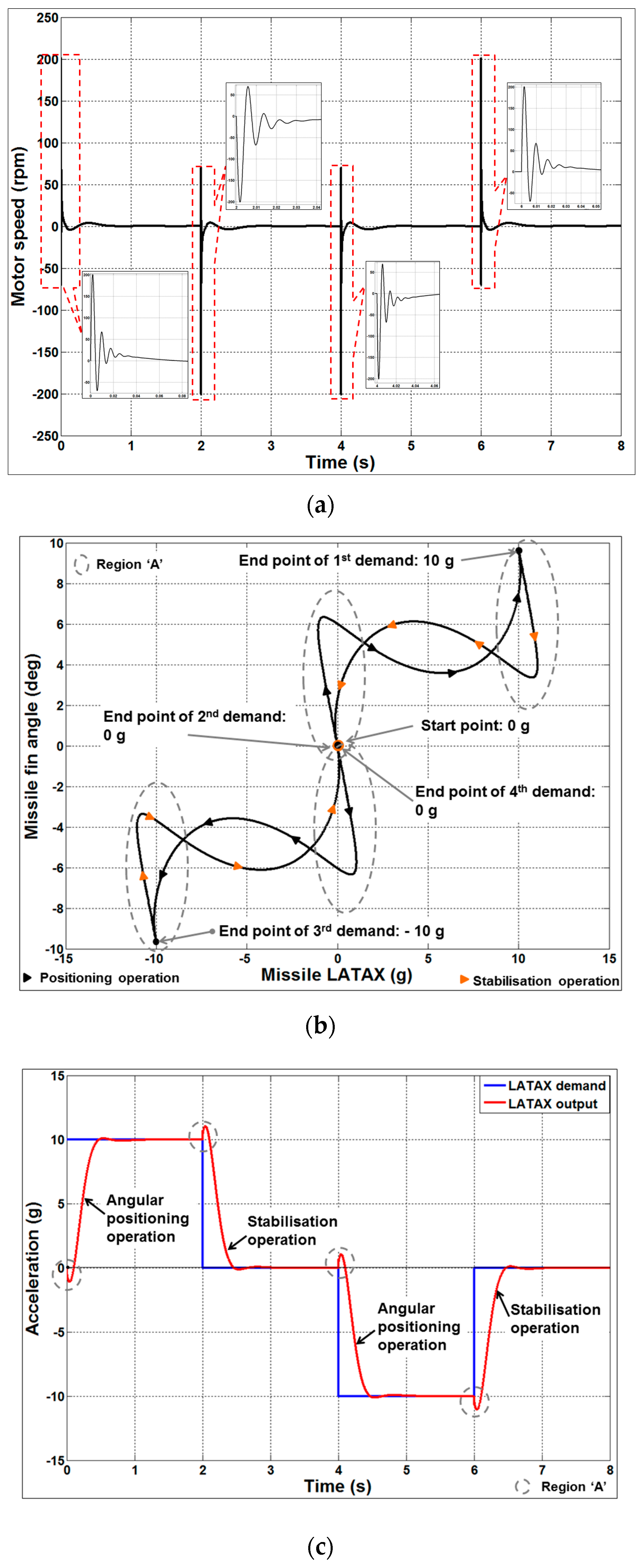
The plots in Figure 12 depict satisfactory performance of the LATAX autopilot with the proposed actuator fin angle for a staircase LATAX demand. In each of the LATAX demands, the actuator supplies the required torque to hold the missile in a given position at Mach 2.0. The effect of zeroes in the autopilot, also known as the non-minimum phase effect (due to the tail fin control), is marked as “Region A”. Thus, it can be observed from the simulation results for various scenarios that the performance of the proposed actuator alone and along with the dual-feedback LATAX autopilot for a tail-fin-controlled missile is satisfactory and operates within the actuator bounds (Figure 8a). It may also be noted that the actuator architecture is functioning satisfactorily for both stabilisation and position control operations and, hence the proposed actuator design can be used for any of the operations.
Equation (12) shows the measured fin angle in relation to the demanded fin angle and the results in Figure 8b and Figure 9d clearly indicate that after any transients the measured angle settles with approximately zero steady-state error to the desired values. In particular, Figure 9d shows the fin angle settling for both the stabilisation and set-point modes of operation. The steady-state errors are not precisely zero due to the numerical gain values. Furthermore, Equation (20), which incorporates Equation (12), does cause an accumulative error in the steady-state values. For example, Figure 10c and Figure 11c show the transient and steady-state agreement for the LATAX measured signal compared to the step demand. Figure 12c shows the transient and steady-state values for both stabilisation and set-point demands which allows the control strategy for repetitive positive and negative LATAX demands to be checked. In practice, due to the complexity of the models, slight imperfections in the steady-state errors, even for the best choice of feedback gains, can become apparent. Hence, in practice, DC gain amplifiers are used to correct for these discrepancies and the gains are tuned to correct the steady-state system LATAX response to values as near as possible to the demanded values. This approach was used in this paper, for a pulsed LATAX input, to generate a set of corrective DC gains in the ratio shown in Equation (20) as .
5. Discussion
The simulation results match well when comparing the demanded (or otherwise idealised) missile lateral acceleration profile shown in Figure 8c and Figure 12c, respectively. The reason for the slight mismatch between demand (blue) and actual (red) is because the missile behaves dynamically. Its response, therefore, lags the demand and shows a “non-minimum” phase behaviour for every step/pulse change. The demand is modelled as a step input and the observed lag is a characteristic of any dynamic system. In Figure 12, the missile characteristics (red line) shows the non-minimum phase behaviour for a step input and a rise time with a zero steady-state error whereupon the two responses match. Based on this observation, it takes the missile approximately 0.3 s to reach steady-state conditions which is acceptable for such systems.
In Figure 9a, the results also are consistent. There is no need for these to agree because in principle one is a subset of the other. To clarify this, the dynamic results for the fin motor speed in relation to the torque represent how speed and torque vary dynamically with respect to time for the staircase input described in Section 4.1.2. Hence, the figures include the direction of the speed versus torque plot as time is evolving. The linear parallel lines are repeatable for different values of input voltage. There are infinite lines for all the voltages starting from 0 V up to 50 V. Furthermore, Figure 8a shows the agreement of the results between the steady-state DC motor linear characteristics for a choice of five representative input voltages (10 V to 50 V) and the dynamical trajectory which includes the arrows so that the time-evolution of the trajectory has a sense of direction.
Hence, to avoid clutter, the graphs are limited to showing some of the linear lines which represent the motor speed versus torque characteristic independent of time, i.e., these are static. Figure 9a shows that the motor speed characteristics (selected linear lines) and the system dynamical motion have a trajectory that does reside within the operational envelope of this specific motor. Hence the dynamic actuator response is within the motor static lines.
6. Conclusions
The load torque feedforward compensation scheme with a dual-switching strategy proposed in this paper has resulted in deriving a rear-fin, direct-drive actuated missile with combined missile airframe dynamics and a LATAX autopilot design. The novelty of having a single model that offers both the missile airframe variables and the electromechanical actuator state variables, including the motor torque (together with the angular position and velocity) in relation to the LATAX a missile can achieve, has resulted in understanding better the parametric relationships when testing a range of potential actuator designs for a missile airframe while being tested for the same flight conditions. This produces a cost-efficient approach in testing the performance of the overall missile LATAX autopilot performance in relation to actuator choice with a reduced need for expensive missile testing. Furthermore, the choice of actuator can be monitored and checked to see if it is operating outside the normal operational boundaries by utilising the steady-state actuator angular speed versus torque characteristics for a range of operational voltages. The performance of the actuator during the missile flights explored in this paper has shown that the fin actuator operates within the steady-state actuator characteristics and therefore can produce the required LATAX airframe demands.
Author Contributions
Bhimashankar Gurav and John Economou conceived the idea. Bhimashankar Gurav, John Economou and Alistair Saddington implemented the model. Bhimashankar Gurav, John Economou, Alistair Saddington and Kevin Knowles contributed to the analysis of the results and writing of the article.
Conflicts of Interest
The authors declare no conflict of interest.
Abbreviations
| Function of ) | |
| B | Frictional constant (Nm/rad/s) |
| Function of (Cmα) | |
| Cmα | Pitching moment coefficient |
| Cmδ | Control moment coefficient |
| Cnα | Normal force coefficient |
| Cnδ | Control force coefficient |
| J | Actuator inertia (kg/m2) |
| Ka | Actuator Back EMF constant (V/rad/s) |
| Kd | Derivative gain |
| Kp | Forward gain |
| Kp1 | Proportional gain (for θd = 0, i.e., stabilisation operation) |
| Kp2 | Proportional gain (for θd ≠ 0, i.e., position operation) |
| Torque sensitivity (Nm/A) | |
| L | Inductance (H) |
| Actuator input power | |
| Ra | Armature resistance (Ω) |
| Actuator torque | |
| Missile fin loading | |
| Airframe Velocity | |
| Actuator armature current | |
| kα | Acceleration feedback gain |
| kf | Forward gain |
| kr | Rate feedback gain |
| Achieved or actual/measured LATAX | |
| Demanded LATAX | |
| Fin actual angle | |
| Fin demanded angle | |
| Actuator angular position | |
| Demanded servo angle | |
| Actuator angular velocity | |
| Function of (Cnα, Cmα, Cnδ, Cmδ) | |
| Function of (Cnα, Cmα, Cnδ, Cmδ) |
References
- Hwang, T.W.; Tahk, M.-J.; Park, C.S. Adaptive sliding mode control robust to actuator faults. Proc. Inst. Mech. Eng. Part G J. Aerosp. Eng. 2007, 221, 129–144. [Google Scholar] [CrossRef]
- Liu, X.; Wu, Y.; Deng, Y.; Xiao, S. A global sliding mode controller for missile electromechanical actuator servo system. Proc. Inst. Mech. Eng. Part G J. Aerosp. Eng. 2014, 228, 1095–1104. [Google Scholar] [CrossRef]
- Tsourdos, A.; White, B.A. Adaptive flight control design for nonlinear missile. Control Eng. Pract. 2005, 13, 373–382. [Google Scholar] [CrossRef]
- Buschek, H. Design and flight test of a robust autopilot for the IRIS-T air-to-air missile. Control Eng. Pract. 2003, 11, 551–558. [Google Scholar] [CrossRef]
- Kim, S.-H.; Kim, Y.-S.; Song, C. A robust adaptive nonlinear control approach to missile autopilot design. Control Eng. Pract. 2004, 12, 149–154. [Google Scholar] [CrossRef]
- Devaud, E.; Siguerdidjane, H.; Font, S. Some control strategies for a high-angle-of-attack missile autopilot. Control Eng. Pract. 2008, 8, 885–892. [Google Scholar] [CrossRef]
- Menon, P.K.; Ohlmeyer, E.J. Integrated design of agile missile guidance and autopilot systems. Control Eng. Pract. 2001, 9, 1095–1106. [Google Scholar] [CrossRef]
- Tahk, M.; Briggs, M.M.; Menon, P.K.A. Applications of Plant Inversion via State Feedback to Missile Autopilot Design. In Proceedings of the 27th Conference on Decision and Control, Austin, TX, USA, 7–9 December 1988; pp. 730–735. [Google Scholar]
- Hirokawa, R.; Koichi, S. Autopilot design for a missile with reaction-jet using coefficient diagram method. In Proceedings of the AIAA Guidance, Navigation and Control Conference and Exhibit, Montreal, QC, Canada, 6–9 August 2001; pp. 1–8. [Google Scholar]
- Shtessel, Y.B.; Tournes, C.H. Integrated higher-order sliding mode guidance and autopilot for dual-control missiles. J. Guid. Control Dyn. 2009, 32, 79–94. [Google Scholar] [CrossRef]
- Mehrabian, A.R.; Roshanian, J. Skid-to-turn missile autopilot design using scheduled eigenstructure assignment technique. Proc. Inst. Mech. Eng. Part G J. Aerosp. Eng. 2006, 220, 225–239. [Google Scholar] [CrossRef]
- Reichert, R.T. Dynamic scheduling of modern-robust-control autopilot designs for missiles. In Proceedings of the Conference on Decision and Control, Brighton, England, UK, 11–13 December 1991; pp. 35–42. [Google Scholar]
- Talole, S.E.; Godbole, A.A.; Kolhe, J.P.; Phadke, S.B. Robust roll autopilot design for tactical missiles. J. Guid. Control Dyn. 2011, 34, 107–117. [Google Scholar] [CrossRef]
- Chwa, D.; Choi, J.Y.; Seo, J.H. Compensation of actuator dynamics in nonlinear missile control. IEEE Trans. Control Syst. Technol. 2004, 12, 620–626. [Google Scholar] [CrossRef]
- Menon, P.K.; Iragavarapu, V.R. Adaptive techniques for multiple actuator blending. In Proceedings of the AIAA Guidance, Navigation and Control Conference and Exhibit, Boston, MA, USA, 10–12 August 1998. [Google Scholar]
- Jiang, J.-P.; Chen, S.; Sinha, P.K. Optimal Feedback Control of Direct-Current Motors. IEEE Trans. Ind. Electron. 1990, 37, 269–274. [Google Scholar] [CrossRef]
- Zhong, H.; Pao, L.; de Callafon, R. Feedforward Control for Disturbance Rejection: Model Matching and Other Methods. In Proceedings of the 24th Chinese Control and Decision Conference (CCDC), Taiyuan, China, 23–25 May 2012; pp. 3528–3533. [Google Scholar]
- Linares-Flores, J.; Reger, J.; Sira-Ramirez, H. Load Torque Estimation and Passivity-Based Control of a Boost-Converter/DC-Motor Combination. IEEE Trans. Control Syst. Technol. 2010, 18, 1398–1405. [Google Scholar] [CrossRef]
- Ruderman, M. Tracking Control of Motor Drives Using Feedforward Friction Observer. IEEE Trans. Ind. Electron. 2014, 61, 3727–3735. [Google Scholar] [CrossRef]
- Low, K.-S.; Zhuang, H. Robust Model Predictive Control and Observer for Direct Drive Applications. IEEE Trans. Power Electron. 2000, 15, 1018–1028. [Google Scholar]
Figure 1.
Missile guidance architecture (Levels 1–3).

Figure 2.
Schematic of the direct drive electric actuator, fin and missile (Level 1).

Figure 3.
Missile LATAX autopilot (Level 2).
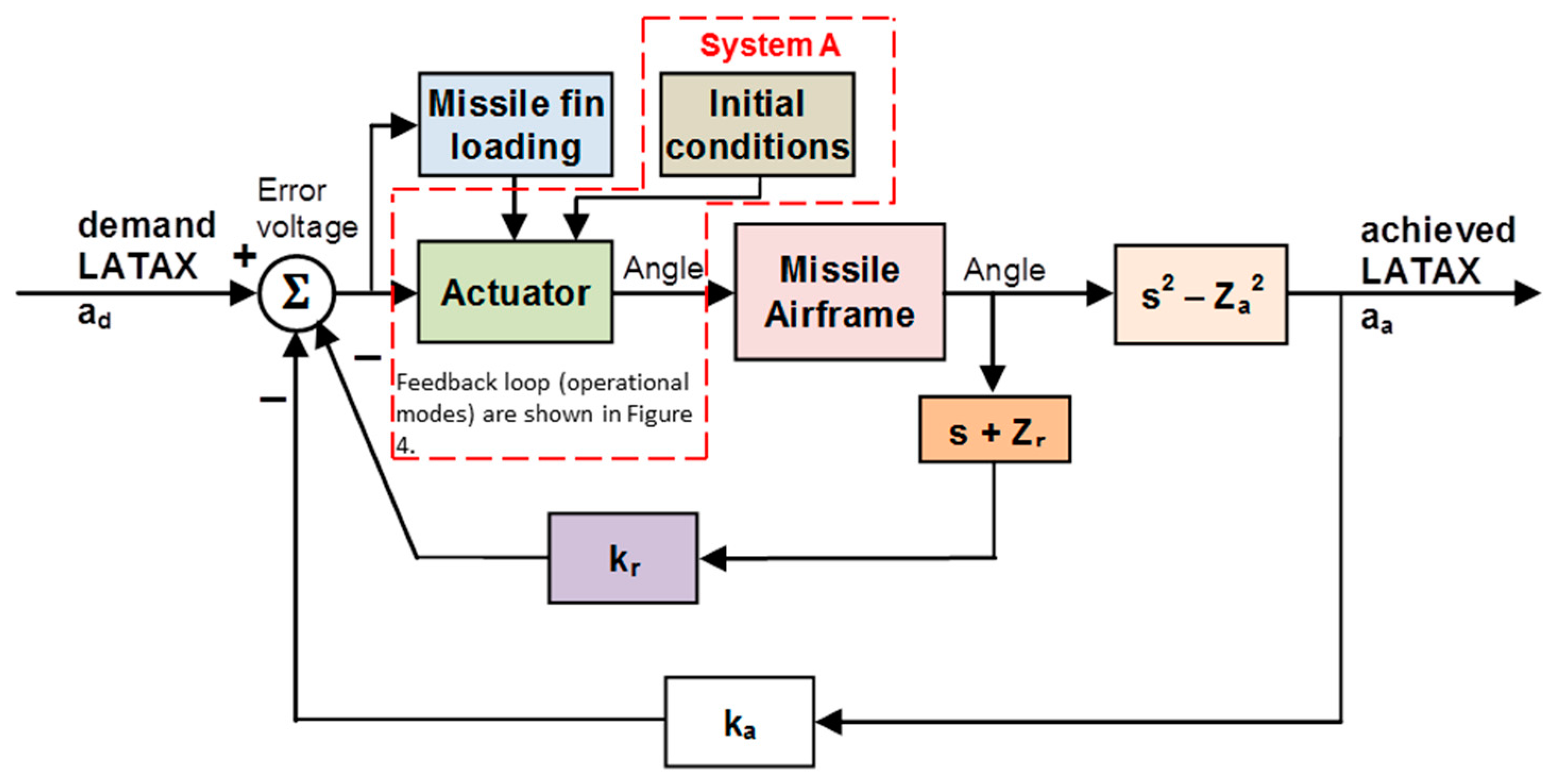
Figure 4.
System A architecture.
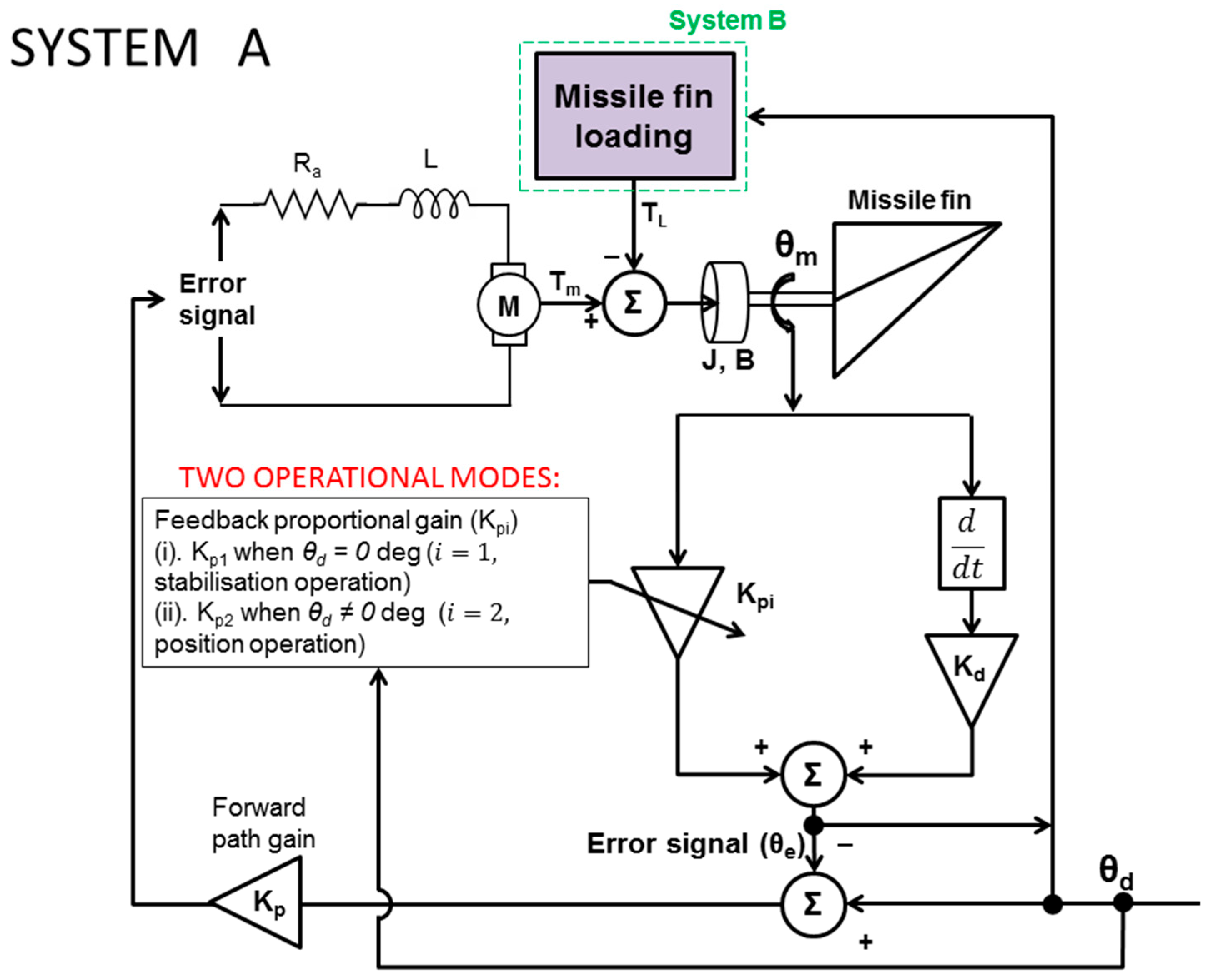
Figure 5.
Missile fin load torque characteristics.

Figure 6.
System B model.

Figure 7.
System parameterization.

Figure 8.
Step input response of the actuator. (a) Steady-state and dynamic characteristics of the actuator for a 15° step input; (b) Angle response of the actuator for a 15° step input; (c) Speed characteristics of the actuator for a 15° step input; (d) Actuator speed with respect to missile fin angle for a 15° step input; (e) Torque characteristics of the actuator for a 15° step input.
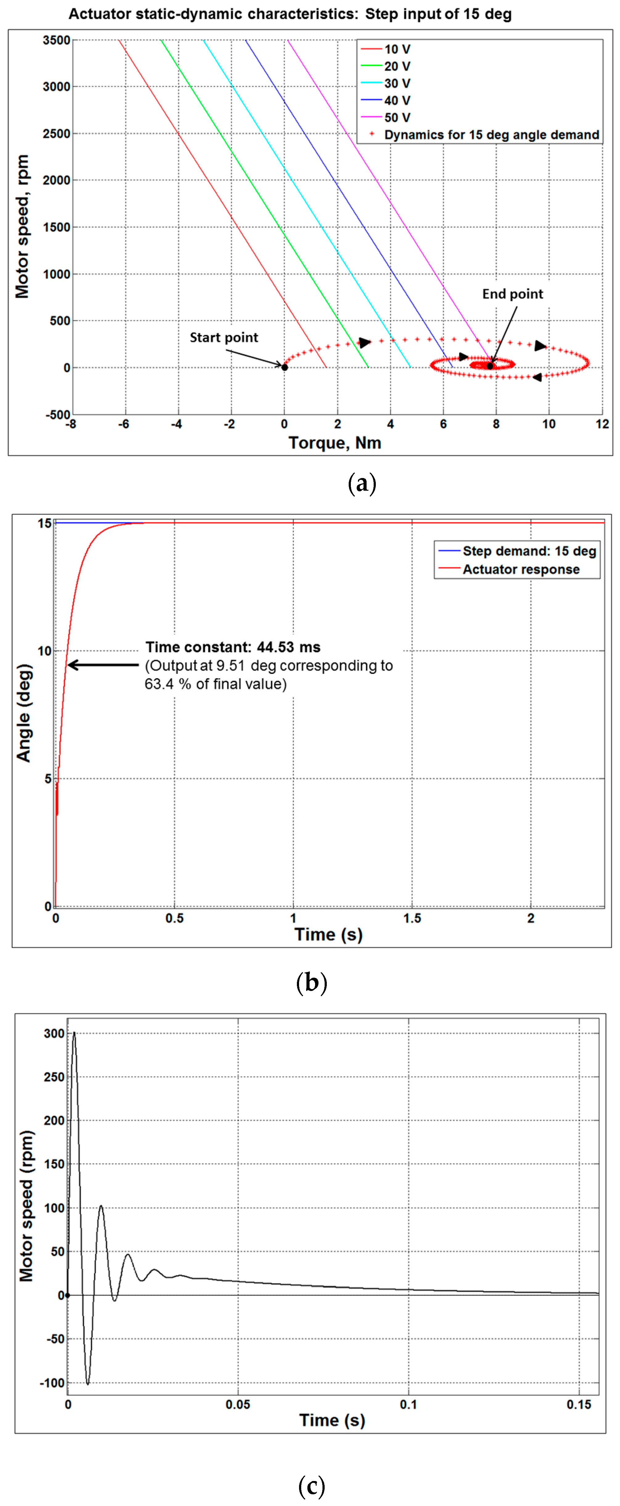

Figure 9.
Staircase input response of the actuator. (a) Steady-state and dynamic characteristics of the actuator for a staircase input; (b) Speed characteristics of the actuator for a staircase input; (c) Actuator speed with respect to missile fin angle for a staircase input; (d) Angle response of the actuator for a staircase input; (e) Torque characteristics of the actuator for a staircase input.

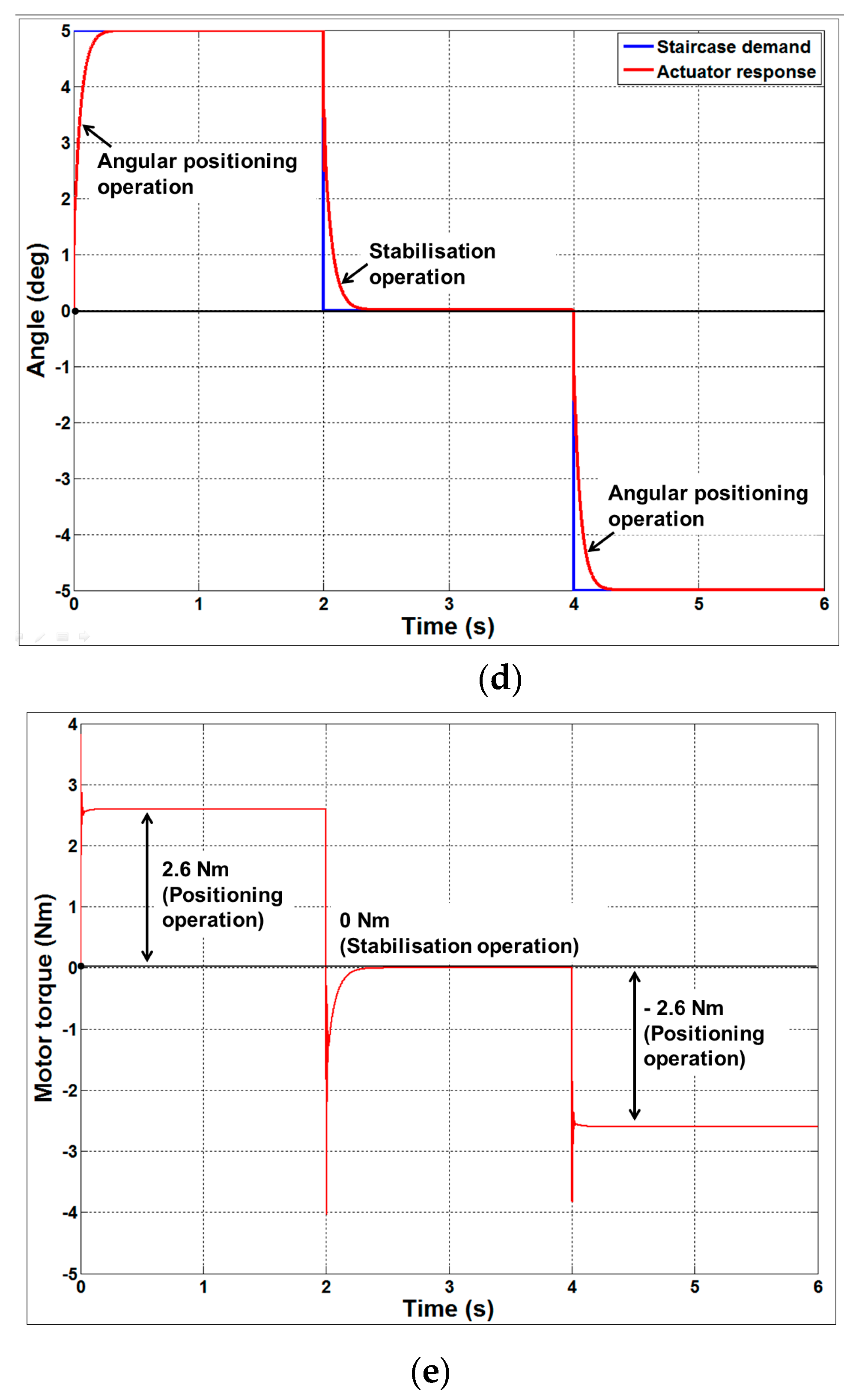
Figure 10.
The 1 g step input response of the autopilot. (a) Speed characteristics of the actuator for a step input of 1 g; (b) Autopilot LATAX with respect to missile fin angle for a step input of 1 g; (c) LATAX response of the autopilot for a step input of 1 g; (d) Torque exerted by the actuator on the missile fin for a step input of 1 g.

Figure 11.
The 10 g step input response of the autopilot. (a) Speed characteristics of the actuator for a step input of 10 g; (b) Autopilot LATAX with respect to missile fin angle for a step input of 10 g; (c) LATAX response of the autopilot for a step input of 10 g; (d) Torque exerted by the actuator on the missile fin for a step input of 10 g.


Figure 12.
Staircase LATAX response of the autopilot. (a) Speed characteristics of the actuator for a staircase LATAX demand; (b) Autopilot LATAX with respect to missile fin angle for a staircase LATAX demand; (c) LATAX response of the autopilot for a staircase LATAX demand; (d) Torque exerted by the actuator on the missile fin for a staircase LATAX demand.


Table 1.
DDEA parameters.
| Parameters | Value |
|---|---|
| Ra | 1.71 |
| L | 0.0212 |
| 0.272 | |
| Ka | 0.1346 |
| J | 2.5 × 10⁻⁴ |
| B | 0.06832 |
| Kd | 0.125 |
| Kp | 50 |
| Kp1 | 0.99944 |
| Kp2 | 4.7443 |
Table 2.
Aerodynamic derivatives.
| Aerodynamic Derivatives | Value |
|---|---|
| Cnα | 23.71 |
| Cmα | −41.22 |
| Cnδ | 10.52 |
| Cmδ | −105.93 |
Table 3.
Feedback gains.
| Feedback Gains for the LATAX Autopilot | Value |
|---|---|
| kr | 0.082 |
| kα | 0.0005 |
| kf | 0.02045 |
Table 4.
Staircase input.
| Staircase Input to the LATAX Autopilot | ||
|---|---|---|
| Operation | Demand (g) | Time Duration (s) |
| Positioning | +10 | 2 |
| Stabilisation | 0 | 2 |
| Positioning | −10 | 2 |
| Stabilisation | 0 | 2 |
© 2017 by the authors. Licensee MDPI, Basel, Switzerland. This article is an open access article distributed under the terms and conditions of the Creative Commons Attribution (CC BY) license (http://creativecommons.org/licenses/by/4.0/).
Share and Cite
MDPI and ACS Style
Gurav, B.; Economou, J.; Saddington, A.; Knowles, K. Multi-Mode Electric Actuator Dynamic Modelling for Missile Fin Control. Aerospace 2017, 4, 30. https://doi.org/10.3390/aerospace4020030
AMA Style
Gurav B, Economou J, Saddington A, Knowles K. Multi-Mode Electric Actuator Dynamic Modelling for Missile Fin Control. Aerospace. 2017; 4(2):30. https://doi.org/10.3390/aerospace4020030
Chicago/Turabian StyleGurav, Bhimashankar, John Economou, Alistair Saddington, and Kevin Knowles. 2017. "Multi-Mode Electric Actuator Dynamic Modelling for Missile Fin Control" Aerospace 4, no. 2: 30. https://doi.org/10.3390/aerospace4020030
Note that from the first issue of 2016, this journal uses article numbers instead of page numbers. See further details here.