Numerical and Experimental Investigations of an Elasto-Flexible Membrane Wing at a Reynolds Number of 280,000

Chair of Aerodynamics and Fluid Mechanics, Department of Mechanical Engineering, Technical University of Munich, 85748 Garching bei München, Germany
*
Author to whom correspondence should be addressed.
†
These authors contributed equally to this work.
Aerospace 2017, 4(3), 39; https://doi.org/10.3390/aerospace4030039
Submission received: 6 July 2017
/
Revised: 24 July 2017
/
Accepted: 24 July 2017
/
Published: 27 July 2017
(This article belongs to the Special Issue Adaptive/Smart Structures and Multifunctional Materials in Aerospace)
Abstract
:This work presents numerical and experimental investigations of an elasto-flexible membrane wing at a Reynolds number of 280,000. Such a concept has the capacity to adapt itself to the incoming flow offering a wider range of the flight envelope. This adaptation is clearly observed in the numerical study: the camber of the airfoil changes with the dynamic pressure and the angle of attack, which permits a smoother and delayed stall. The numerical results, obtained from Fluid Structure Interaction (FSI) simulations, also show that the laminar-turbulent transition influences the aerodynamic characteristics of the wing, as it directly affects the pressure distribution on the membrane and the geometry of the airfoil. Two different turbulence models were therefore tested. Furthermore, experimental investigations are considered in this paper to estimate the precision of the FSI simulations. It appears that the FSI study overestimates the lift coefficient, and the drag coefficient is undervalued, which can be explained by dynamic calibration of the model. Nevertheless, the velocity field obtained with the hot-wire anemometry system shows good agreement on the upper side of the model. The membrane deflection measurements also appear to be consistent with the expected geometry of the deformed airfoil from the FSI simulations.
1. Introduction
“Morphing”, defining the ability to transform the shape or structure and therefore having the capability to take one of various distinct forms, has received considerable attention in recent years [1,2,3,4]. Although many devices have been based on the idea of form-variable geometries, the concept of morphing has recently become a new trend. There is no formal definition to characterize a morphing wing, but the general idea should be understood as a smooth and continuous shape change and flexibility. Morphing is often related to a smart, or an adaptive, or an active, or a reconfigurable wing. Smart, because the wing could be composed of smart materials; adaptive, because the wing adapts itself to the incoming flow; active, because the wing could be directly controlled with actuators; and reconfigurable, because wing geometry could be changed [3]. The main goals of such concepts are to improve efficiency and enlarge the flight envelope of an aircraft: therefore, one configuration could have the capacity to accomplish different missions under different conditions.
In 2007, Rodriguez listed different research topics concerning actual morphing technologies [3]. Among others, the “Morphing Aircraft Structure” program funded by the DARPA (Defense Advanced Research Projects Agency) successfully developed the Lockheed Martin Morphing configuration [5] and the NextGen MFX-1 aircraft [6]. The first concept has the capacity to fold itself from a loiter configuration into a dash geometry, reducing the wing area to extend the Mach number range where the aircraft does not experience aeroelastic instabilities. The second concept is designed with a morphing wing based on an innovative flexible skin, which allows the wing to stretch smoothly and continuously from one shape to another. The wing has one degree of freedom, as the area change and the sweep angle are interdependent. Nevertheless, between two extreme configurations, the wing area can be changed by approximately 40%. In line with the idea of morphing the wingspan, the University of Maryland initiated research on a pneumatic telescopic wing for unmanned aerial vehicles in 2002 [7]. The wing integrated a pressurized telescopic spar able to extend in the spanwise direction, which could provide an alternative form of roll control. As wingspan directly affects the lift produced by the wing, roll control can be achieved by creating a difference in span between the two half wings. The telescopic wing was successfully tested at four different spans and it was found that at maximum deployment, it incurred a larger drag and a reduced lift-to-drag when compared to its solid fixed wing counterpart. As the drag penalty came mostly from the seam of the wing sections, future works will focus on improving the manufacture of the wing.
Wingspan or sweep changes are two examples of the different methods that are included in the word morphing. In this paper, the considered morphing characteristics are about the camber change of a wing. Camber morphing has already been investigated in several studies [8,9,10,11,12,13]. The variation of camber can be used to steer an airplane but also to improve flying capabilities by influencing the amount of lift and drag produced by an airfoil. Yokozeki and Sugiura [8] investigated a variable camber morphing airfoil by using a corrugated structure. The study used a Wortmann FX63-137 airfoil (maximum thickness ratio 13.7%, camber ratio 5.89%) as wing model with a morphing section (as trailing edge) situated after 69% of the chord. The morphing trailing edge is made with corrugated structures, which have a high load bearing capacity in the direction perpendicular to corrugation but are very flexible in the corrugation direction. Therefore, the corrugation was made in the chord direction to enable the camber change. The corrugated structures were moved using a wire, which was connected to the trailing edge and to an actuator; activating the actuator permitted tension in the wire, which resulted in downward deformation of the trailing edge. It was found that the lift of the wing could be increased by using an increase of the camber. Beguin [9,10] showed the same results by analyzing a morphing membrane wing. Furthermore, it could be seen that the membrane’s flexibility permitted the airfoil to adapt itself to the surrounding flow field by naturally redistributing the pressure difference on the upper side and the lower side of the membrane [9,10,11,12,13]. This capacity of adaptivity resulted in a delay of the stall to higher angles of attack and could produce an increase of the camber and a reduction in the thickness, which could provide more favorable lift-to-drag characteristics.
The wing considered in this paper is a morphing wing made with a highly extensible, anisotropic elastic membrane, which enables the change of the camber and the thickness of the airfoil section. The concept is to use the high-compliance, low-weight and adaptive characteristic of the membrane: on the one hand, this could permit an alleviation of the loads and, on the other hand, this could improve flight capabilities with passive control of the produced amount of lift and drag. Different experiments have already been performed [9,10,14], which showed the possibility to delay the stall to higher angles of attack by means of such a morphing system. Nevertheless, as analysis of this kind of concept only started in the 1970s, high-quality numerical simulations are required Interaction between fluid and structure needs to be simulated in order to reproduce the interdependency between the flow and the membrane. In this paper, a numerical Fluid Structure Interaction (FSI) investigation of an elasto-flexible membrane wing is presented and compared to experimental tests, which were performed to draw conclusions about the plausibility and the accuracy of the numerical method. The focus on the paper was on the modeling of the interaction between the flow and the membrane. Therefore the phenomenon of hysteresis was not taken into account during the experiments: they were performed by starting with the smallest angle of attack to the highest one with a break between two different angles of attack. As the simulations were done independently of each other, a comparison between experiments and simulations could have been done directly.
The paper is organized as follows: in the first part, the experimental set up is presented with the experimental measurement techniques. Then, the set up of the numerical investigations is described with an emphasis on the fluid set up. Finally, the results are discussed in the last part with a comparison between numeric results and experiments.
2. Experimental Configuration and Measurement Techniques
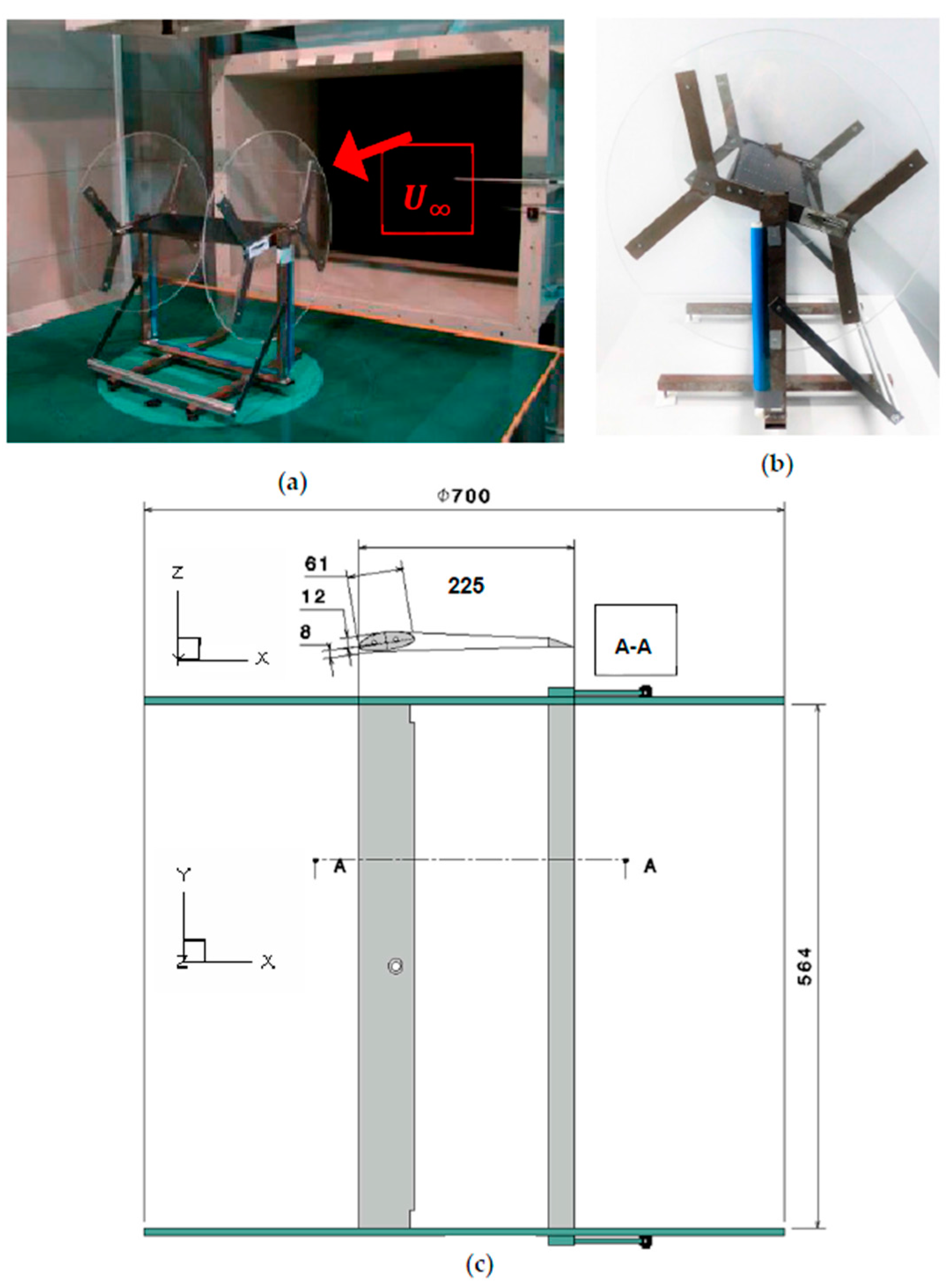
The experimental tests were carried out in wind tunnel facility B of the Chair of Aerodynamics and Fluid Mechanics at the Technical University of Munich (TUM-AER). The wind tunnel, depicted in Figure 1a, has an open rectangular test section, which is 2.85 m long, 1.2 m wide and 1.55 m high. The facility can generate incoming flow velocities of up to 65 m/s with freestream turbulence levels below 0.4%. In order to deeply investigate the elasto-flexible membrane wing model, the experimental tests included force measurements, planar/surface flow field measurements and membrane deformation measurements.
2.1. Experimental Model
The wind tunnel model investigated in this paper consists of a quasi-2D model represented in Figure 1. The concept is based on rigid leading and trailing edge, built as spars to support the membrane, which is wrapped around them. The leading edge spar is built with an asymmetric double elliptical section developed to reduce the pressure gradient at the beginning of the suction side of the leading edge [10]. In comparison with a cylindrical spar, the peak of suction is considerably reduced, which lowers the possibility of flow separation. The trailing edge spar is relatively thick in order to avoid deflection under aerodynamic loads. The membrane used for the wing surface is a product of the manufacturer Eschler Textil GmbH situated in Switzerland (Sevelen, Switzerland). It is made of a highly extensible anisotropic elastic fabric coated on one side with a rubber layer ensuring impermeability. The mechanical properties of the membrane should be determined with a biaxial tensile test [15]. For a first draft, basic uniaxial tests were performed to get an idea of the magnitude of the moduli of elasticity. The moduli of elasticity were measured in Béguin’s thesis [10] and are shown in Figure 2. The stress-strain curves were approximated with a linear function: as the model is used in the weft direction, the considered modulus of elasticity is equal to 2.18 MPa. The wing was held by a support where endplates were also settled; see Figure 1. The endplates of circular planform were used to limit the 3D flow effects produced by the wing tip vortices. The endplates had a diameter of three times the airfoil chord and were made of Plexiglas to provide optical access to the deformation of the membrane. The experimental wing had an overall span of 0.564 m and a nominal chord of 0.220 m, giving an aspect ratio of AR ≈ 2.56. As Béguin [9,10] showed, the pre-stress of the membrane is a critical parameter in such a concept as it has a direct impact on the deflection of the membrane and, consequently, on the aerodynamic characteristics of the wing. It is, therefore, crucial to know the pre-stress of the membrane for the tests. In order to pre-stress the membrane, the wing was made with a moveable trailing edge spar, which enables the user to set a pre-stress by introducing an initial elongation. In this paper, the considered initial elongation is equal to 2.27% of the chord, which corresponds to an operative chord of c = 0.225 m and an operative aspect ratio of AR ≈ 2.51.
2.2. Force Measurements
The lift, the drag and the pitching moment of the wing were measured using an external six component aerodynamic balance set under the test section of the wind tunnel. The deformation of the strain gauge resulting from aerodynamic loading on the wing provided the forces acting on the model. Since the elasto-flexible membrane wing was fixed to the support, the aerodynamic loads measured during the tests were the forces acting on the entire model. It was therefore necessary to know the forces acting on the support to isolate the respective loads of the wing. A so-called dynamic calibration was performed using a “dummy wing” to measure the forces of the support. The “dummy wing” consisted of a wing whose geometry was similar to the elasto-flexible membrane wing. As the purpose of the dynamic calibration was to measure the forces acting on the support, the “dummy wing” was not fixed to the support but held with the traversing unit between the endplates to simulate real flow conditions. When testing the membrane wing, the forces and moments of the support were subtracted from the overall loads providing only the loads acting on the elasto-flexible membrane wing. Force measurements were conducted for different angles of attack from 0° to 18° at 20 m/s, which corresponds to a Reynolds number of 280,000. Repeated measurements indicated an average deviation equal to ∆CL = ±0.8% and ∆CD = ±4%.
2.3. Flow Field Measurements
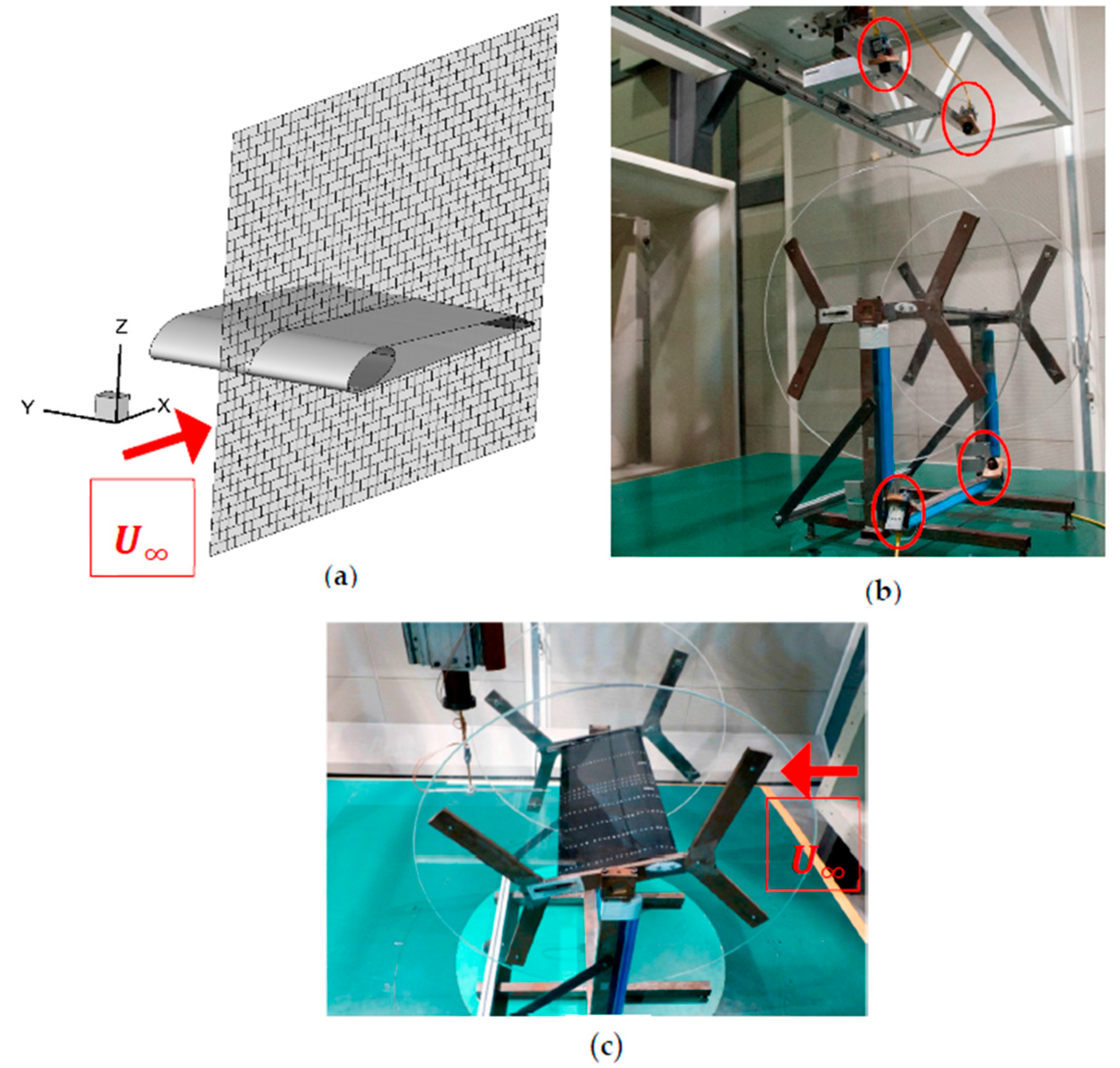
In order to analyze the flow field, a hot-wire anemometry system (HWA) was used. This system permitted measurement of the mean flow velocities and the turbulence intensities around the wing. The measurements were carried out with miniature cross-wire probes on the basis of a look-up table technique for constant temperature anemometry including temperature correction. For each point, 19,200 samples were recorded, which corresponded to a measurement time of 6.4 s as a sampling rate of 3000 Hz was used. During one measurement cycle, two components of the velocity were recorded: the axial velocity component U and the orthogonal velocity component W. The considered axes are depicted in Figure 3a. The plane where the velocity was measured was located in the middle of the wingspan as can also be seen in Figure 3a, where the flow topology is supposed to be closer to a 2D flow. The traversing unit was used to shift the HWA within a grid resolution of ∆x,z = cr/22 in the x and z directions and a refinement of ∆z = cr/73 near the membrane. As shown in Figure 3c, measurements were conducted on the upper side of the membrane.
2.4. Membrane Deflections Measurements
In order to measure membrane deflection, a stereophotogrammetry technique developed at the TUM-AER by Béguin, based on direct linear transformation (DLT), was used [10,16]. Four cameras (FlowSense 2M) were placed on the traversing unit with a 45° angle of separation between their optical axes, as shown in Figure 3b. The cameras recorded instantaneous measurements of the reflective markers stuck on the membrane, which are illustrated in Figure 3b along the wing span. The cameras have a resolution of 1600 × 1200 pixels, which in conjunction with the image optics and the distance to the model, makes the size of the measurement x-y plane 208 × 156 mm2.
The basis of the stereophotogrammetry theory is to calculate the 3D coordinates of the reflective markers from two photos of the model taken with two cameras. Using the DLT equations and a calibration test, the 2D coordinates of the images can be transformed into 3D coordinates [16]. The calibration of the test consisted, of moving the cameras or a two-dimensional grid of markers defining the x-y plane by means of the traversing unit to several z positions. As the positions of the markers inside the x-y plane are known and the z positions are chosen, a volume defined by [xmin xmax, ymin ymax, zmin zmax] can be calibrated. Reconstructing the position of the reference points inside the object space using the transformation parameters obtained during the calibration indicated an average in the error measurement of 0.13 mm per pixel. The measurements were conducted in two sections: the upper and the lower sides of the membrane were investigated at the same time.
2.5. Test Cases and Conditions
The quasi-2D elasto-flexible membrane wing was investigated in order to measure the forces, the flow field and the membrane deflections under different freestream conditions. The considered freestream conditions are summarized in Table 1. The force measurements were conducted using an aerodynamic balance situated under the test section of the wind tunnel for the dynamic pressure of 230 Pa. The range of angles of attack was from 0° to 18°, with a rough step of 2° and a fine step of 1° around the stall region. The flow field measurements were conducted with a hot-wire anemometry system for the same dynamic pressure at two different angles of attack, namely 6° and 15°. The hot-wire anemometry system was controlled with the traversing unit of the wind tunnel. In order to stay consistent, membrane deflection was also measured at 230 Pa for four angles of attack, namely 0°, 6°, 10° and 15°.
3. Numerical Modeling
The numerical investigation was performed using a coupling between the Unsteady Reynolds-Averaged Navier-Stokes Computational Fluid Dynamics (U-RANS CFD) solver ANSYS CFX and the Finite Element Method (FEM) structural solver ANSYS APDL. In order to be consistent with the experimental investigations, the simulations were computed for the Reynolds number of 280,000. The flow around the wing and the deformation of the membrane were simulated for different angles of attack, namely from 0° to 18°. In the following sections, the set up in both solvers will be presented.
3.1. Wing Geometry
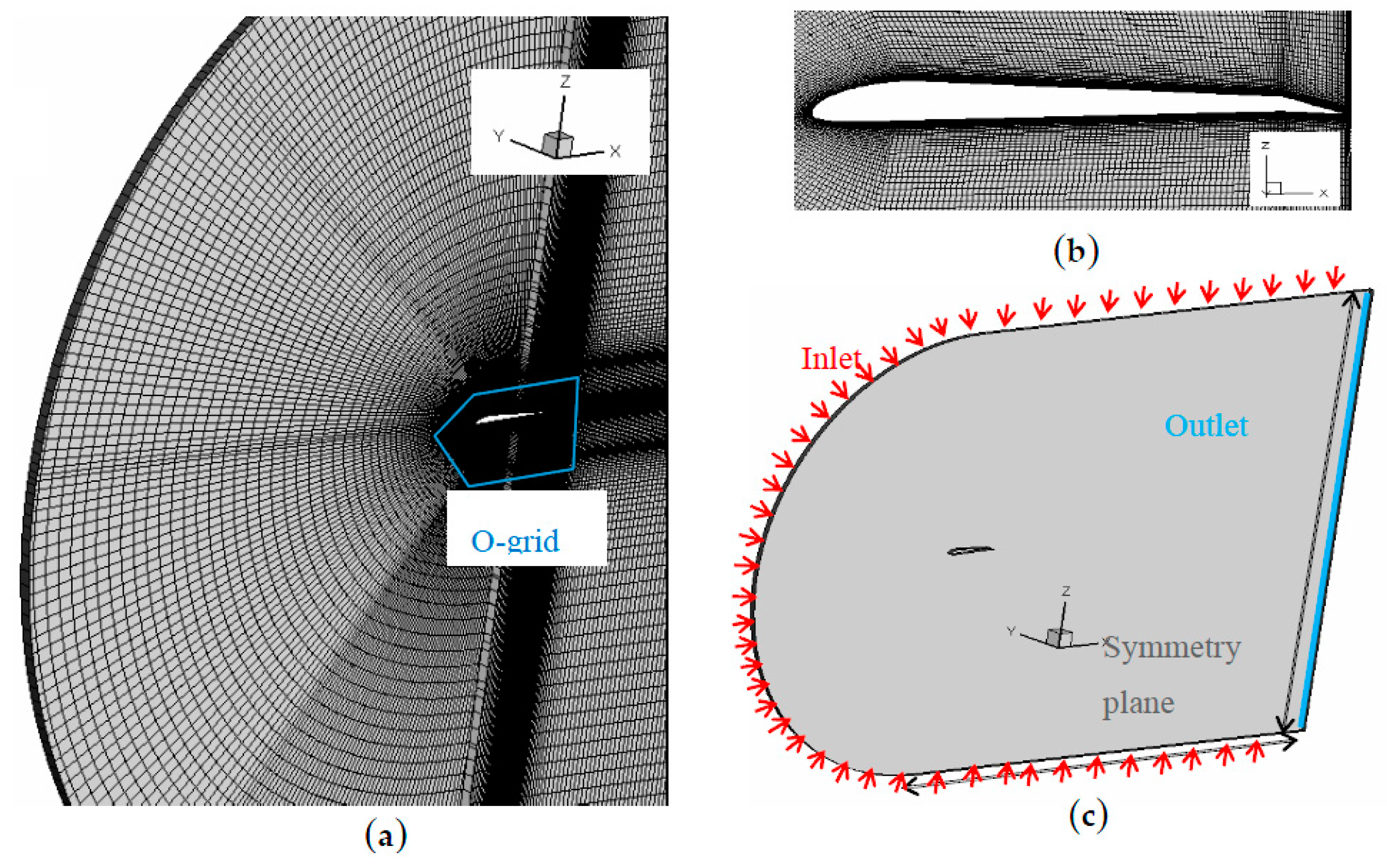
The numerical model investigated in this paper is a reproduction of the experimental wing model in 2D with an extrusion in the third direction. As the interaction between the fluid and the structure is not negligible, two models have to be considered: one for the flow and another for the structure. The geometry of the airfoil for the structural analysis consisted of three different parts: a double elliptical spar for the leading edge, a triangular spar for the trailing edge, and the membrane wrapped around both spars. The fluid domain is a C domain, which is depicted in Figure 4c. It can be seen that the 2D model has an extrusion in the y direction, as the solver ANSYS CFX cannot consider planar interpretation. Nevertheless, the length of the extrusion is equal to 1% of the chord length, which is negligible compared to the other lengths.
3.2. Grid Generation and Grid Independency Study
C-grid blocking was used to create a structured mesh to represent the fluid domain. The C-grid is created according to the following: upstream of the leading edge, the fluid domain is around 5 times the chord length (5 m) and downstream of the trailing edge, the domain is 10 times the chord length (2 m). An O-grid is also created around the airfoil to refine the boundary layer, as can be seen in Figure 4a,c. A value of y+ = 1 is used to assure an accurate resolution of the viscous sublayer, which corresponds to a distance of the first node of around 0.05 mm from the airfoil.
A grid sensitivity study was undertaken: four meshes were tested to know the influence of the mesh on the results and to find a suitable grid for the numerical investigation. The different characteristics of the grids are described in Table 2.
The results of the grid sensitivity study are shown in Figure 5, where the lift coefficient of the wing is plotted for different angles of attack and for the four different meshes. Only the results for the grid sensitivity with the k-ω SST model coupled with the transition γ-Reθ model are considered in this paper [14]. As expected, the results were sensitive to the grid refinement: if the fine mesh is considered a reference grid, the coarse and medium meshes appeared to overestimate the lift coefficient values. The errors for the lift coefficient between the coarse and fine on the one hand, and the medium and the fine on the other hand were around 20% and 6%, respectively. Nevertheless, the results obtained with the extra fine mesh appear similar to the results with the fine mesh: the biggest difference was obtained for AOA = 15° with an error of 3%. Therefore, the fine grid was chosen to perform the numerical investigations.
3.3. Fluid Structure Interaction Set Up
3.3.1. Structural Set Up
The structural geometry is, as mentioned in Section 3.1, composed of three parts: the leading edge, the trailing edge and the membrane, conformal to the experimental model. Both spars were set as fixed solids in order to accurately represent the FSI simulations in comparison with the experiments. The membrane is, as mentioned in Section 2.1, an anisotropic material, whose mechanical properties are different in the weft and the warp directions. The respective E-moduli for the weft and the warp directions are 2.18 and 1.01 MPa respectively. As the considered model is supposed to be 2D, it was decided for the present investigation to model the membrane as an isotropic material with an E-modulus equal to the E-modulus of the membrane in the chord direction, namely 2.18 MPa, and a Poisson coefficient of 0. As only one node was used in the extrusion direction and both extreme faces were defined as symmetry planes, the deformation of the membrane would be 2D in the x-z plane of the system.
3.3.2. Fluid Set Up
The Reynolds number considered in this work is equal to 280,000. According to the Mayle correlation [17], the percentage of laminar flow relative to the chord length is estimated to be not negligible: it is supposed to be more than 5% of the length of the wing. It was already showed that the laminar-turbulent transition considerably affects the behavior of the elasto-flexible membrane as it directly influences the pressure distribution on the wing and, consequently, the deformation and the geometry of the wing [10,18]. Therefore, two different flow models are investigated in unsteady mode in this paper: the k-ω SST model coupled with the γ-Reθ transition model [19,20], which is used for the transition phenomenon, and the k-ω SST model without transition modeling. The unsteady mode was chosen as it permitted to stabilize the structural solver by allowing a smoother change in the pressure on the membrane. The time step for both fluid models was set as 0.008 s for a total time of 2 s. The velocity at the inlet followed a ramp function until 1 s and was then set as constant to 20 [m/s]. The transition model was adapted at each time step to have a better precision on the pressure distribution on the membrane. Furthermore, the fluid was set as incompressible as the considered Mach number was lower than 0.3 and was supposed to be isothermal. The residual criteria were set following the rule that the maximal value of all the residuals should be lower than 10−4. A second order upwind scheme for the convection terms was used and all the diffusion terms were discretized with the second order central difference scheme.
3.4. Test Cases and Conditions
Fluid Structure Interaction simulations were used to numerically analyze the elasto-flexible membrane wing. The numerical model considered in this paper is a 2D reproduction of the experimental geometry presented in Section 2.1. The U-RANS CFD solver ANSYS CFX was used to solve the Navier-Stokes equations for the flow, and the FEM solver ANSYS APDL was used to simulate the deformation of the membrane. The coordinator ANSYS MFX was adopted to ensure the exchange of information between the two solvers. As mentioned in Section 3.2, the FSI investigations were performed using two different flow models at Re = 280,000, namely the k-ω SST model coupled with the γ-Reθ transition model and the k-ω SST model.
4. Results and Discussion
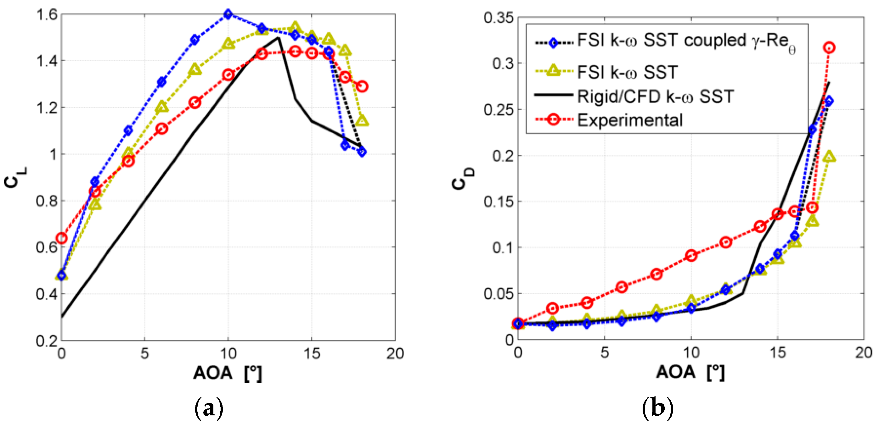
The lift and drag coefficients of the FSI simulations are plotted in Figure 6. The FSI results with the SST k-ω model are symbolized as green stars, the FSI results with the k-ω SST model coupled with the γ-Reθ model are symbolized as blue diamonds and the results for the rigid case are plotted in a continuous black line. The lift and drag coefficient from the FSI are the converged values of each characteristic obtained after 2 s of simulation. In the next figures and the following sections, the pressure coefficient distribution and the deformation along the wing for the different fluid models are illustrated and explained. Furthermore, the associated flow field obtained with hot-wire anemometry are plotted and correlated to FSI simulations.
4.1. The Elasto-Flexible Membrane Wing Compared to Its Rigid Counterpart
Different characteristics of the camber-morphing wing are shown in Figure 6 by comparing the aerodynamic coefficients to those obtained with the rigid case. The simulations of the rigid geometry were performed using the same fluid mesh but with the CFD solver only.
On the one hand, the results of the rigid geometry were usual for an airfoil: the lift coefficient increased linearly with the AOA until it reached the maximum value of 1.5 for AOA = 13°; then the lift coefficient decreased abruptly in connection with a sudden increase in the drag coefficient. Such characteristics indicate that the rigid airfoil stall occurred for an AOA around 13°. The numerical analysis for the rigid geometry was done using the k-ω SST model. On the other hand, the aerodynamic behavior of the elasto-flexible membrane was fairly different. If the FSI results obtained with the k-ω SST model are considered, the lift-AOA curve can be considered linear for small AOA (<10°) but the values of the lift coefficient are much higher than those of the rigid geometry. At AOA = 0°, the elasto-flexible membrane wing had a lift coefficient of 0.48 compared to 0.3 for the rigid airfoil. As the membrane offers the possibility to adapt itself to the flow, the camber of the airfoil increased for positive angles of attack increasing the lift coefficient of the wing. Furthermore, between an AOA of 12° to 17°, the lift coefficient of the elasto-flexible membrane wing featured a continuous transition from slightly positive to negative gradients whereas it dropped abruptly in the rigid case. In the same range of AOA, the drag coefficient increased continuously without any abrupt change in contrast to its rigid counterpart. The adaptivity of the membrane permitted the flow to stay attached up to larger angles of attack offering a delayed and smoother stall.
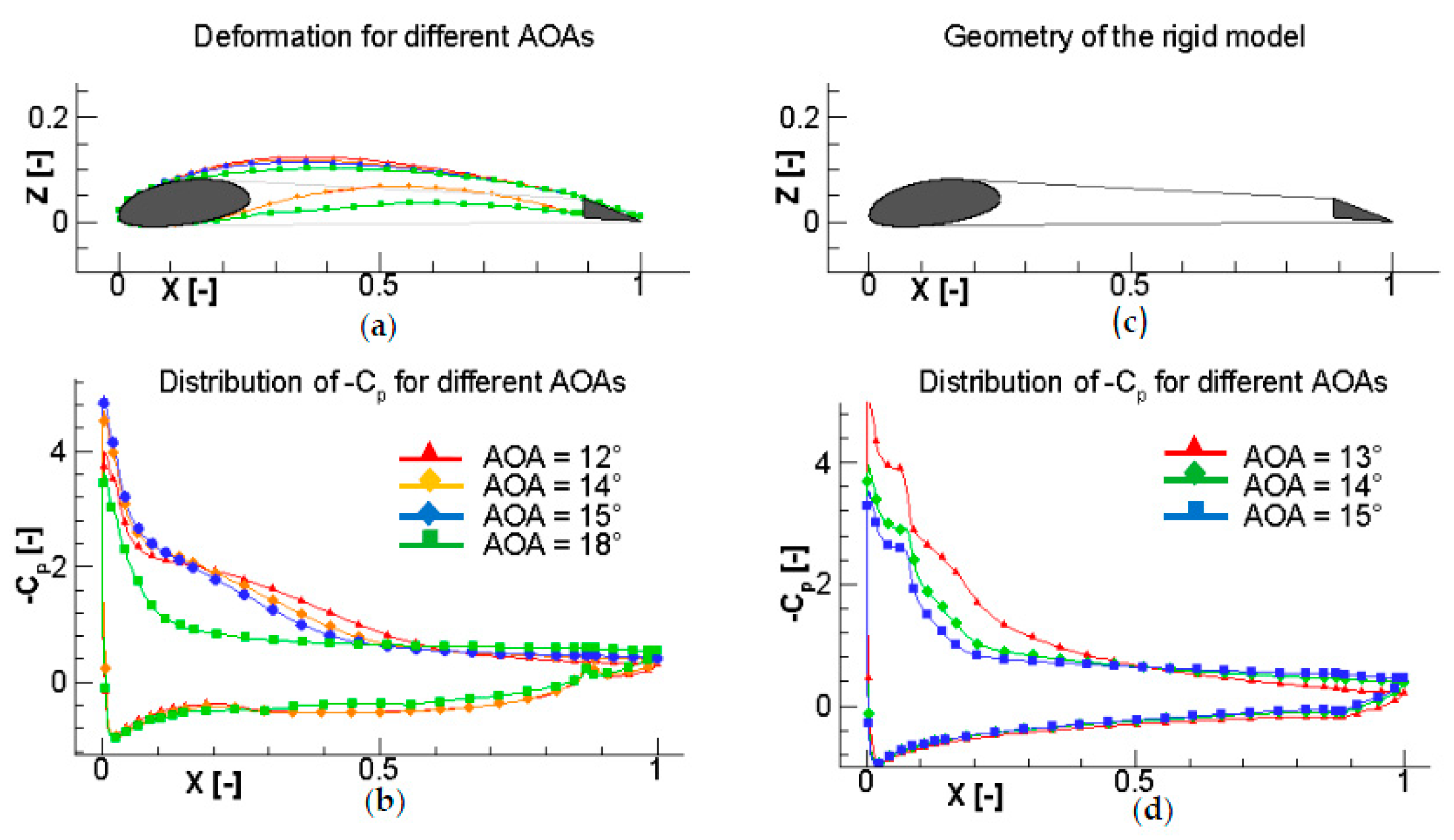
In order to explain the continuous behavior of the stall, Figure 7 represents the deformation of the elasto-flexible membrane and the associated pressure coefficient at different angles of attack in the stall region. The position of the flow separation for the elasto-flexible membrane and the rigid case shifted to the nose of the wing when the angle of attack got higher. For the FSI k-ω SST model, the separation occurred on the upper surface at X/c = 55% at AOA = 12° and at X/c = 40% for AOA = 15°, whereas it occurred at X/c = 10–20% for the rigid case. This position shifted to the nose of the wing for the rigid case as well, but a completely separated flow occurred for smaller AOA, as it can be seen in Figure 7c. The flow was completely separated at AOA = 18° for the elasto-flexible membrane wing, whereas for the rigid case (Figure 7d), it happened at AOA = 15°. This delay caused by the adaptivity of the wing explains the smoother and later stall observed in the force measurement figures.
Figure 7 also shows that the deformation of the membrane got smaller when the angle of attack increased. This phenomenon is due to the same facts mentioned above: when the flow separation on the upper side occurs, the pressure gradient is less favorable for a positive deformation of the membrane. As the separation point moves towards the leading edge when the AOA increases, the deformation of the membrane gets smaller when the angle of attack increases.
4.2. Influence of the Transition Modeling
The CL- and CD-AOA curves obtained with the k-ω SST model coupled with the γ-Reθ transition model in contrast to the k-ω SST model are symbolized in Figure 6 as blue diamonds and green stars, respectively. In both cases, the adaptivity of the elasto-flexible membrane wing was observed taking the above description into account.
Nevertheless, the first significant difference between the two models occurred from AOA = 2° to AOA = 10° in the linear region of the CL-AOA curve: the lift coefficient of the wing is clearly higher for the transitional modeling than for the fully turbulent one. In order to better understand the difference between the models, Figure 8 and Figure 9 illustrate the pressure coefficient along the wing and the turbulence intensity Tu defined from the turbulence kinetic energy. In Figure 9, three different angles of attack, namely 0°, 6° and 15°, were chosen to analyze the difference between the models. Those three angles of attack were chosen taking into account the CL- and CD-AOA curves: 0° as both models have similar coefficients, 6° as the coefficients are significantly different and 15° as both models have once more similar coefficients. For AOA = 0°, it was observed that the boundary layer had the same nature in both models, which resulted directly in the same CL and CD (Figure 6). For AOA = 6°, the difference came from the laminar-turbulent transition situated on the upper side of the wing. The transition occurred around X/c = 55% and was directly observed in Figure 8 by means of the pressure coefficient. The value for -Cp was higher for the transition model, which resulted in a higher lift coefficient and slightly higher deformation. For AOA = 15°, the transition point moved to the nose of the leading edge, and both boundary layers were similar. The pressure distributions along the wing for both models were therefore comparable, which resulted in CL values close to each other.
The second difference was that the stall appeared for a higher AOA (17°) in the fully turbulent case than in the transitional one. The fully turbulent boundary layer had a steeper velocity gradient, which delayed the flow separation; therefore, the stall appeared for higher AOA in the k-ω SST model.
4.3. Experimental Investigations Compared to FSI Simulations
The plausibility of the FSI simulations was investigated by comparing different parameters with experiences described in part 2. First, the aerodynamic force coefficients CL and CD are plotted in Figure 6. Then, the deformation of the membrane is depicted in Figure 10; the upwind behind the model if depicted in Figure 11 and finally the flow field is shown in Figure 12 and Figure 13 for specific AOAs.
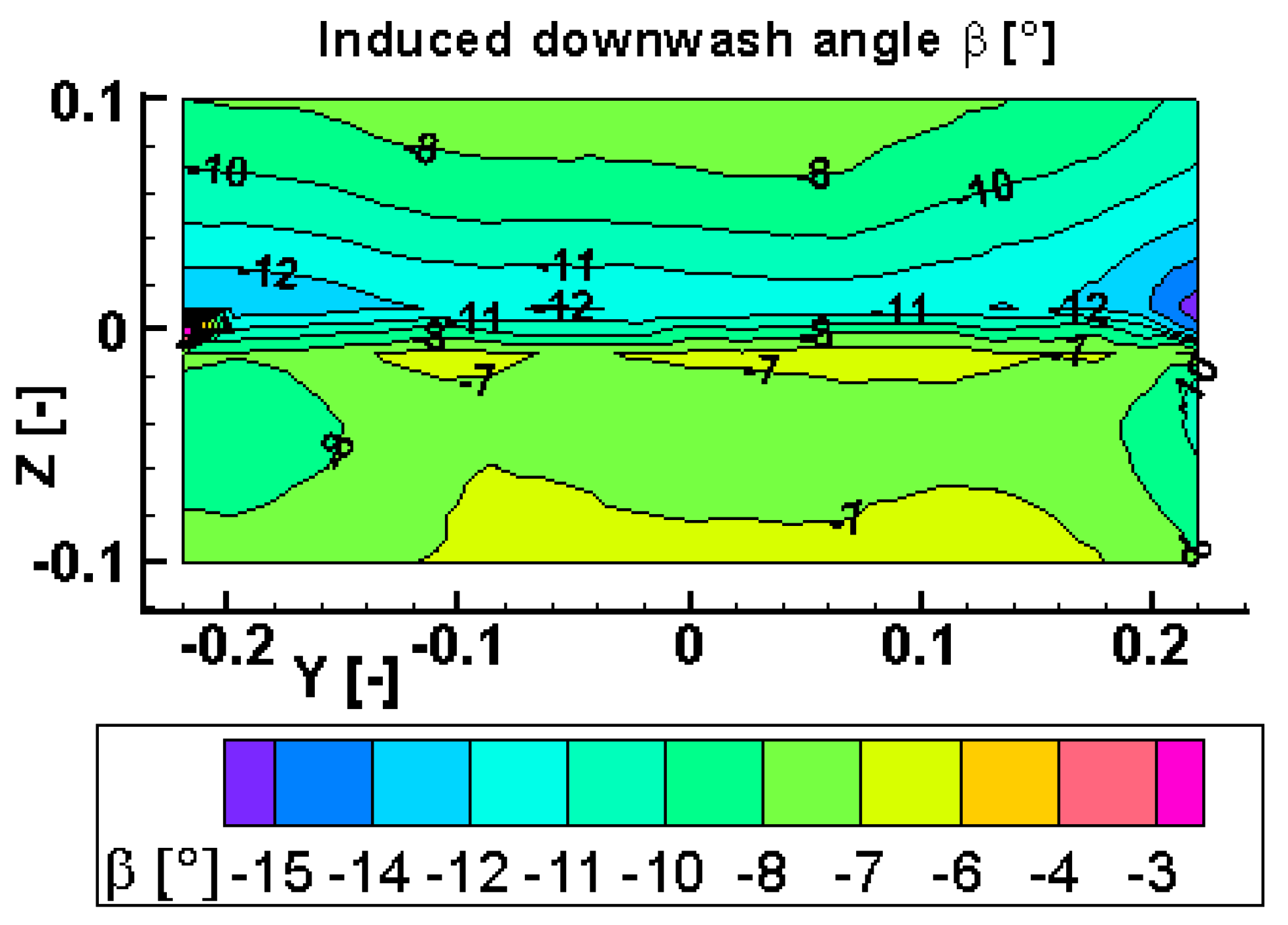
Figure 6 represents the CL- and the CD-AOA curves. The results for the experiments are depicted as red circles. It can be seen that the aerodynamic coefficients obtained in the wind tunnel tests were different from the coefficients obtained with the U-RANS/FEM simulations. On the one hand, the experimental lift coefficient values were lower and, on the other hand, the experimental drag coefficient values were higher. One hypothesis to explain the first issue comes from the 3D effects during the experiments: the endplates should minimize the tip vortices of the wing but the flow observed was not completely uniform over the wingspan. Downwash was measured behind the model between the endplates using hot-wire anemometry and is depicted in Figure 11. It can be seen that 3D effects at the tips of the wing exist, which can explain a lower lift coefficient; see Figure 6. This phenomenon needs to be directly linked with the deformation of the membrane, which is analyzed in more detail in the following sections. The second issue is due to the dynamic calibration of the experimental model. As the drag of the structure was not negligible compared to the drag of the wing, the error of ∆CD = ±4% during the measurement had a significant effect on the results.
The phenomenon observed around AOA = 10° in the FSI simulations performed with the transition model, was not observed in the experiments: the slope of the CL-AOA curve stayed constant until the smooth stall at AOA = 17°. Furthermore, the results obtained with the k-ω SST model were closer to the experiments. Therefore, in order to compare the FSI simulations with the experiments, only the results obtained with the k-ω SST model will be considered in the following.
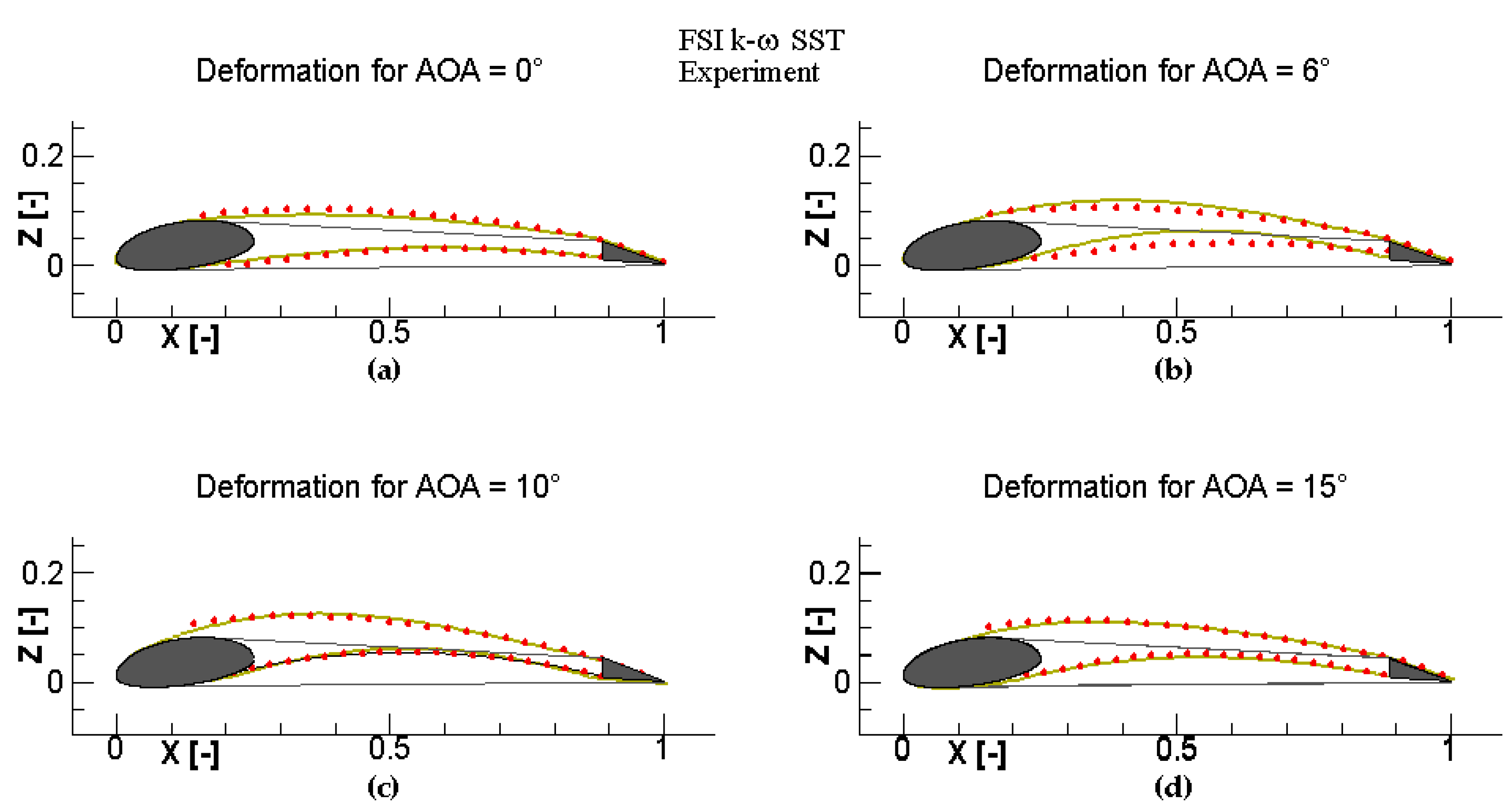
As mentioned above, the aerodynamic forces are directly linked to the deformation of the membrane. The deformation is depicted in Figure 10; the experiments are marked as red circles and the final geometry obtained with the FSI simulations is drawn with a continuous green line. The deformation of the membrane was measured for four different angles of attack at Re = 280,000, namely AOA = 0°, 6°, 10° and 15°. As shown, the deformation obtained during the experiments was close to the final geometry of the FSI simulations. Nevertheless, some small disparities could be observed, which directly resulted in differences in the CL-AOA curve. For AOA = 0°, the deformation obtained in the experiment was higher on the upper side of the membrane, which resulted in a higher lift coefficient. The opposite phenomenon was observed for AOAs = 6°, 10° and 15°: the deformation was higher for the FSI simulations, which caused a higher lift coefficient in the FSI results. The disparities were small but had a significant influence on the forces of the system. However, the general trend seen in the experiments can be reproduced by the FSI simulations: on the one hand, when the angle of attack becomes higher, the camber of the profile increases, which permits higher lift coefficients. On the other hand, the stall region appears smooth.
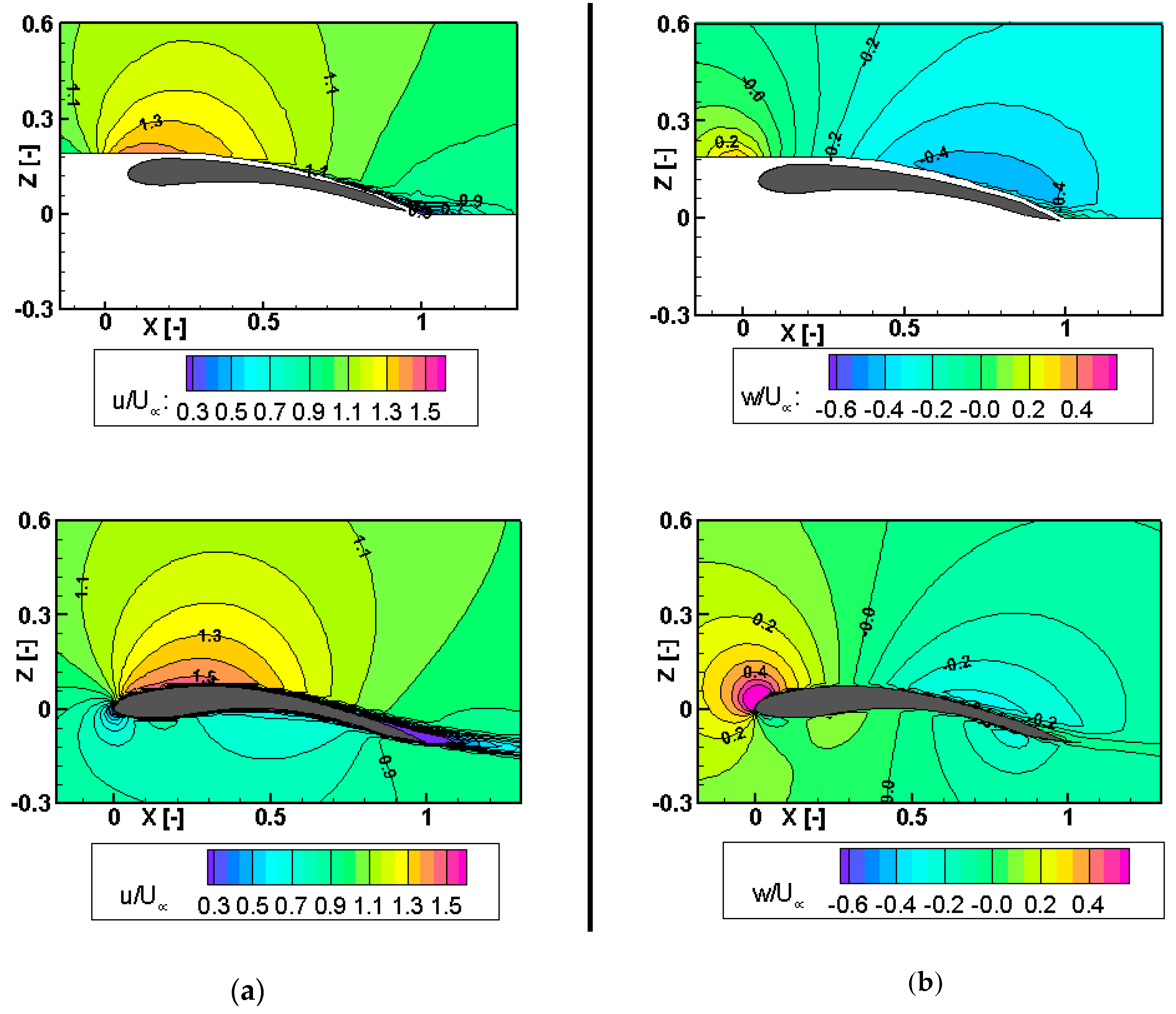
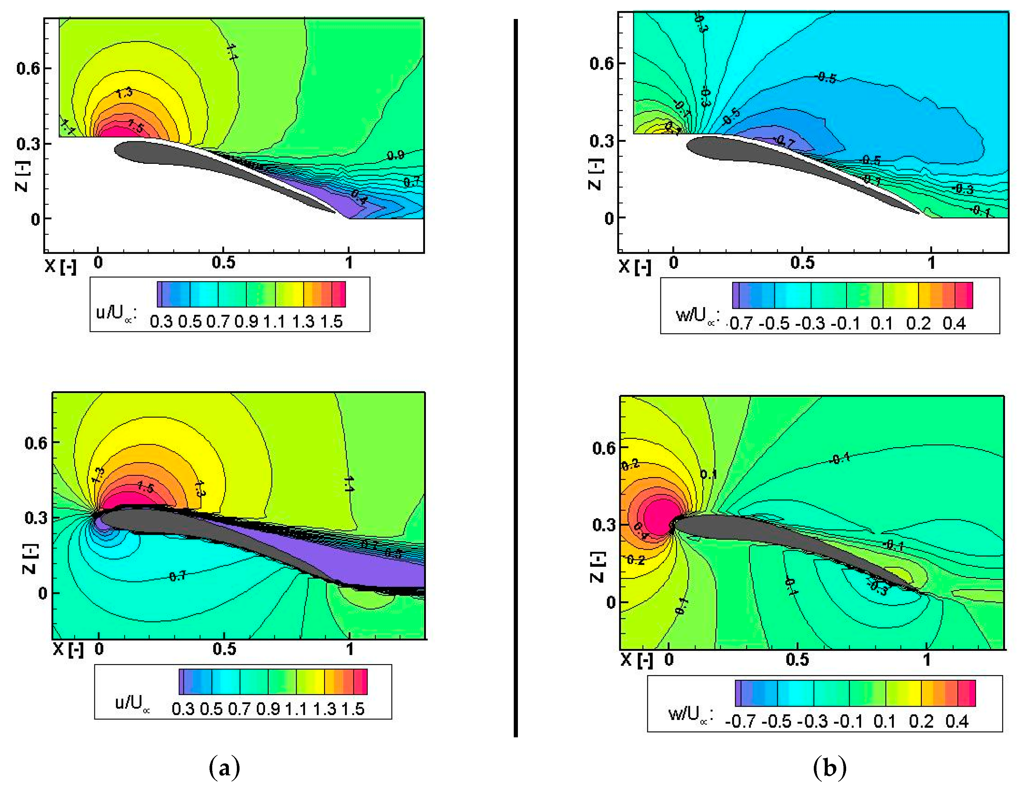
The flow visualization, namely the U component and W component of the velocity of the flow field in the experiments, can be seen in Figure 12 and Figure 13 on the top of the figures. In each figure, the U and W components of the velocity obtained with the FSI are plotted on the lower side. Considering that the field close to the airfoil could not be measured because of the security distance between the membrane and the sensor, the flow around the airfoil appeared congruent with the one obtained with the FSI simulations, but with some disparities due to the differences in the deformation of the membrane.
The flow in the trailing edge region differed from the FSI. The region of high velocity and the wake region appeared smaller in the experiments than in the FSI simulations. The first phenomenon could be explained by the disparities in the deformations of the membrane. Even though the differences were small, they had an important influence on the forces of the system, which is seen in the flow environment as well. The camber obtained with the simulation was a bit higher, which resulted in the following: The flow could accelerate over a longer distance along the upper side of the airfoil and stayed attached longer. Furthermore, the wake region downstream the airfoil was much smaller in the wind tunnel compared to the FSI simulations. This characteristic is consistent with the hypothesis of the 3D effects of the experimental model. The downwash flow produced by the 3D effect decreased the local AOA, resulting in a later stall observed in the aerodynamic force measurements and causing a smaller wake region behind the wing. This reduction of the wake region was observed at AOA = 6° but was even more intense at AOA = 15°. Fluid Structure Interaction simulations were used to numerically analyze the elasto-flexible membrane wing.
5. Conclusions
An elasto-flexible membrane wing was investigated to quantify the benefits of such a design compared to its rigid counterpart. An experimental investigation including flow measurements, aerodynamic force measurements and deformation measurements was compared to 2D Fluid Structure Interaction simulations performed with a coupling between CFD/U-RANS and FEM methods. The results showed that the experimental prototype exhibited 3D effects, which affected the behavior of the system. Furthermore, the comparison of the membrane deformation between FSI simulations and experiments showed some disparities, which affected the flow and resulted in differences in the aerodynamic forces obtained within the experiment.
Nevertheless, FSI and experimental tests illustrated the typical characteristics and benefits of an elasto-flexible membrane wing compared to its rigid counterpart. As the membrane was able to balance the pressure on the upper and lower sides of the wing, the flow could stay attached longer and did not induce abrupt changes in the stall region. Therefore, the stall region appeared smoother and was delayed to higher angles of attack. Furthermore, the camber of the profile increased with positive angles of attack, resulting in a higher lift coefficient. However, this advantage of the configuration should be analyzed carefully as one of the limitations of the elasto-flexible membrane wing is that when the camber is too high, it leads to an earlier detached flow phenomenon and therefore lower CL and higher CD.
Finally, two different turbulence models were used for the numerical FSI investigations: the k-ω SST model and the k-ω SST model coupled with the γ-Reθ transition model. Neither one reproduced the experimental data exactly, but a bigger difference was observed in the transition model as the laminar region of the boundary layer affected the deformation of the airfoil. The main difference between the modeling with and without a transition occurred between AOA = 2°–10° where a laminar separation bubble migrated from the trailing edge to the leading edge in the transitional fluid model. The transition model offered a profile, which provided more lift because of its more cambered geometry at Re = 280,000, which in this case was favorable for the aerodynamics of the wing. The second difference was that the stall appeared for much higher AOAs in the fully turbulent case than in the transitional one. The fully turbulent boundary layer had a steeper velocity gradient, which delayed the flow separation.
As the 2D FSI investigation could not reproduce the experimental tests exactly, future work will focus on developing a 3D FSI model. We will also focus on the variation of the pre-stress of the membrane and its mechanical properties such as Young’s modulus. Those parameters appear important regarding their effect on the aerodynamic properties of the wing and the precision of the simulations.
Acknowledgments
The support of these investigations by the German Research Foundation (Deutsche Forschungsgemeinschaft) is gratefully acknowledged. Furthermore, the authors would also like to thank ANSYS for the possibility to use their softwares.
Author Contributions
Julie Piquee performed the experiments and analyzed the data. Julie Piquee and Christian Breitsamter wrote the paper.
Conflicts of Interest
The authors declare no conflict of interest.
Abbreviations
The following abbreviations are used in this manuscript:
| CFD | Computational Fluid Dynamic |
| U-RANS | Unsteady Reynolds-Averaged Navier-Stokes |
| FSI | Fluid Structure Interaction |
| AR | Aspect Ratio, - |
| c | Chord, m |
| E | Young’s Modulus, MPa |
| Re | Reynolds Number, - |
| AOA | Angle of Attack, ° |
| X, Y, Z | Dimensionless System Coordinates, - |
| y+ | Dimensionless Wall Distance, - |
| U∞ | Freestream Velocity, m/s |
| U | x Component of the Velocity, m/s |
| W | z Component of the Velocity, m/s |
| ∆cr | Grid Resolution, mm |
| q∞ | Freestream Dynamic Pressure, Pa |
| CP; CL; CD | Pressure Coefficient, -; Lift Coefficient, -; Drag Coefficient, - |
| Tu | Turbulence Intensity, - |
References
- Weisshaar, T.A. Morphing Aircraft Systems: Historical Perspectives and Future Challenges. J. Aircr. 2013, 50, 337–353. [Google Scholar] [CrossRef]
- Vasista, S.; Tong, L.; Wong, K.C. Realization of Morphing Wings: A Multidisciplinary Challenge. J. Aircr. 2012, 49, 11–28. [Google Scholar] [CrossRef]
- Rodriguez, A.R. Morphing Aircraft Technology Survey. In Proceedings of the 45th AIAA Aerospace Sciences Meeting and Exhibit, Reno, NV, USA, 8–11 January 2007. [Google Scholar]
- Moorhouse, D.; Sanders, B.; von Spakovsky, M.; Butt, J. Benefits and Design Challenges of Adaptive Structures for Morphing Aircraft. Aeronaut. J. 2006, 110, 157–162. [Google Scholar] [CrossRef]
- Ivanco, T.G.; Scott, R.C.; Love, M.H.; Zink, S.; Weisshaar, T.A. Validation of the Lockheed Martin Morphing Concept with Wind Tunnel testing. In Proceedings of the 48th AIAA/ASME/ASCE/AHS/ASC Structures, Structural Dynamics, and Materials Conference, Honolulu, HI, USA, 23–26 April 2007. [Google Scholar]
- Flanagan, J.S.; Strutzenberg, R.C.; Myers, R.B.; Rodrian, J.E. Development and Flight Testing of a Morphing Aircraft, the NextGen MFX-1. In Proceedings of the 48th AIAA/ASME/ASCE/AHS/ASC Structures, Structural Dynamics, and Materials Conference, Honolulu, HI, USA, 23–26 April 2007. [Google Scholar]
- Samuel, J.B.; Pines, D. Design and Testing of a Pneumatic Telescopic Wing for Unmanned Aerial Vehicles. J. Aircr. 2007, 44, 1088–1099. [Google Scholar] [CrossRef]
- Yokozeki, T.; Sugiura, A.; Hirano, Y. Development of Variable Camber Morphing Airfoil Using Corrugated Structure. J. Aircr. 2014, 51, 1023–1029. [Google Scholar] [CrossRef]
- Beguin, B.; Breitsamter, C.; Adams, N. Aerodynamic Investigations of a Morphing Membrane Wing. AIAA J. 2012, 50, 2588–2599. [Google Scholar] [CrossRef]
- Beguin, B. Development and Analysis of an Elasto-Flexible Morphing Wing. Ph.D. Thesis, Chair of Aerodynamics and Fluid Mechanics, Technische Universität München, Munich, Germany, 2014. [Google Scholar]
- Stanford, B.; Viieru, D.; Albertani, R.; Shyy, W.; Ifju, P. A Numerical and Experimental Investigation of Flexible Micro Air Vehicle Wing Deformation. In Proceedings of the 44th AIAA Aerospace Sciences Meeting and Exhibit, Reno, NV, USA, 9–12 January 2006. [Google Scholar]
- Hu, H.; Tamai, M.; Murphy, J.T. Flexible-Membrane Airfoils at Low Reynolds Numbers. J. Aircr. 2008, 45, 1767–1778. [Google Scholar] [CrossRef]
- Ifju, P.; Jenkins, D.; Ettinger, S.; Lian., Y.; Shyy, W.; Waszak, R.M. Flexible-Wing-Based Micro Air Vehicles. In Proceedings of the Confederation of European Aerospace Societies Aerodynamics Conference, Cambridge, UK, 10–12 June 2002. [Google Scholar]
- Piquee, J.; Breitsamter, C. Numerical Analysis of an Elasto-Flexible Wing Configuration Using Computational Fluid Structural Simulations. In Proceedings of the VI International Conference on Textile Composites and Inflatable Structures Structural Membranes 2015, Barcelona, Spain, 19–21 October 2015. [Google Scholar]
- Uhlemann, J.; Stranghoener, N.; Schmidt, H.; Saxe, K. Effects on Elastics Constants of Technical Membranes Applying the Evaluation Methods of MSAJ/M-02–1995. In Proceedings of the Membrane 2011—5th International Conference on Textile Composite and Inflatable Structures, Barcelona, Spain, 5–7 October 2011. [Google Scholar]
- Luhmann, T.; Robson, S.; Kyle, S.; Harley, I. Close Range Photogrammetry, 1st ed.; Whittles Publising: Caithness, UK, 2006. [Google Scholar]
- Mayle, R.E. The Role of Laminar-Turbulent Transition in Gas Turbine Engines. ASME Trans. J. Turbomach. 1991, 113, 509–537. [Google Scholar] [CrossRef]
- Lian, Y.; Shyy, W. Laminar-Turbulent Transition of a Low Reynolds Number Rigid or Flexible Airfoil. AIAA J. 2007, 45, 1501–1513. [Google Scholar] [CrossRef]
- Menter, F.R.; Langtry, R.B.; Likki, S.R.; Suzen, Y.B.; Huang, P.G.; Völker, S. A Correlation-Based Transition Model Using Local Variables–Part I: Model Formulation. J. Turbomach. 2006, 128, 413–422. [Google Scholar] [CrossRef]
- Menter, F.R.; Langtry, R.B.; Likki, S.R.; Suzen, Y.B.; Huang, P.G.; Völker, S. A Correlation-Based Transition Model Using Local Variables–Part II: Test Cases and Industrial Applications. J. Turbomach. 2006, 128, 423–434. [Google Scholar] [CrossRef]
Figure 1.
(a) Experimental model installed in the wind tunnel test section; (b) Experimental model; (c) Sketch of the experimental model (unit in mm).
Figure 1.
(a) Experimental model installed in the wind tunnel test section; (b) Experimental model; (c) Sketch of the experimental model (unit in mm).

Figure 2.
Description of the membrane material: stress-strain curves obtained from unidirectional tensile tests, from [10].
Figure 2.
Description of the membrane material: stress-strain curves obtained from unidirectional tensile tests, from [10].
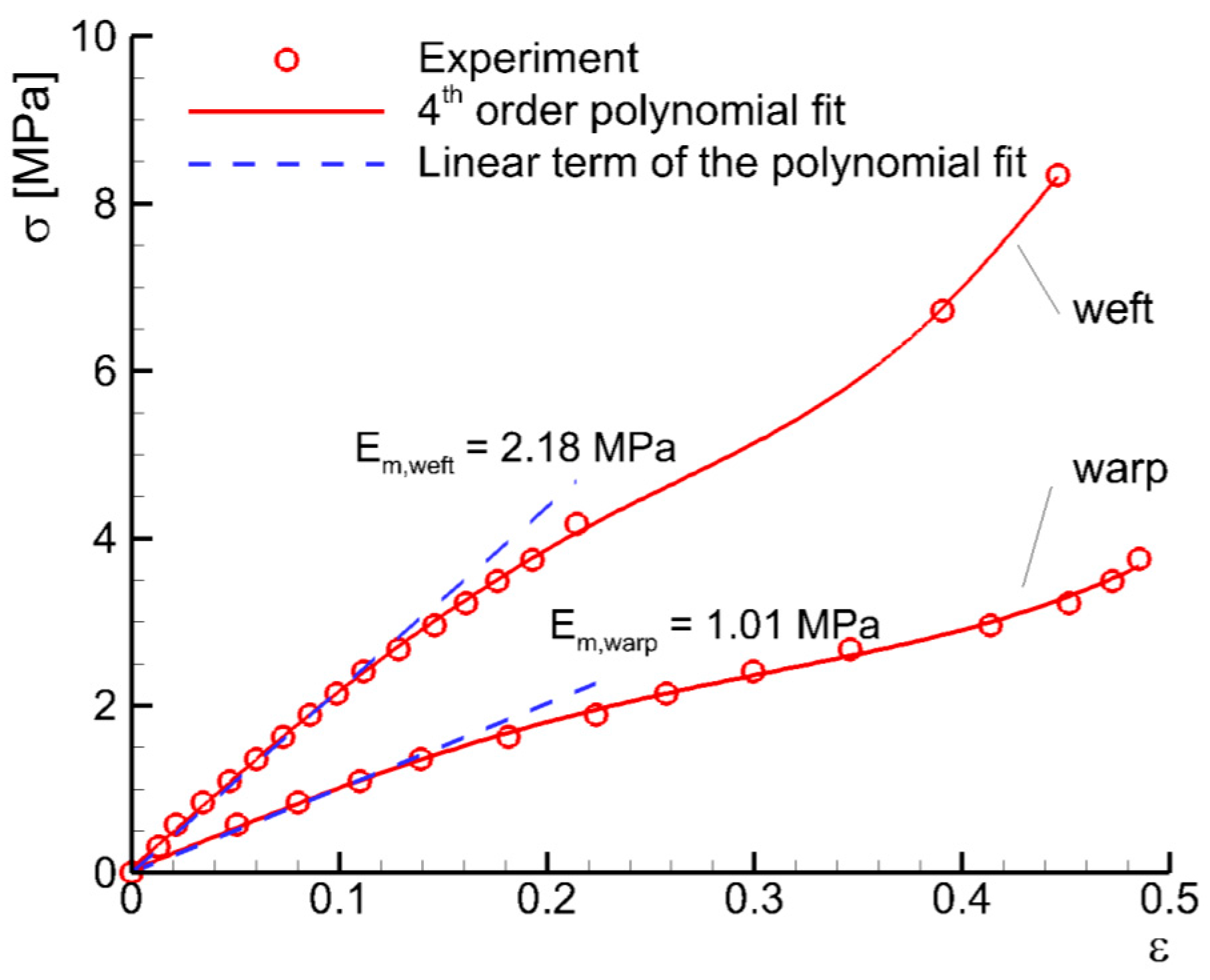
Figure 3.
(a) Experimental plane for the hot-wire measurements (upper side) and the photogrammetry; (b) Set up of the photogrammetry with the four cameras circled in red (2 on the upper side, 2 on the lower side); (c) Set up of the experimental model installed in the wind tunnel test section with the hot-wire anemometry system.

Figure 4.
(a) Quasi-2D fluid mesh; (b) Details of the O-grid around the airfoil; (c) Boundary conditions used for the fluid set up.
Figure 4.
(a) Quasi-2D fluid mesh; (b) Details of the O-grid around the airfoil; (c) Boundary conditions used for the fluid set up.

Figure 5.
Grid independency study: lift coefficient evolution for the different grid resolutions.
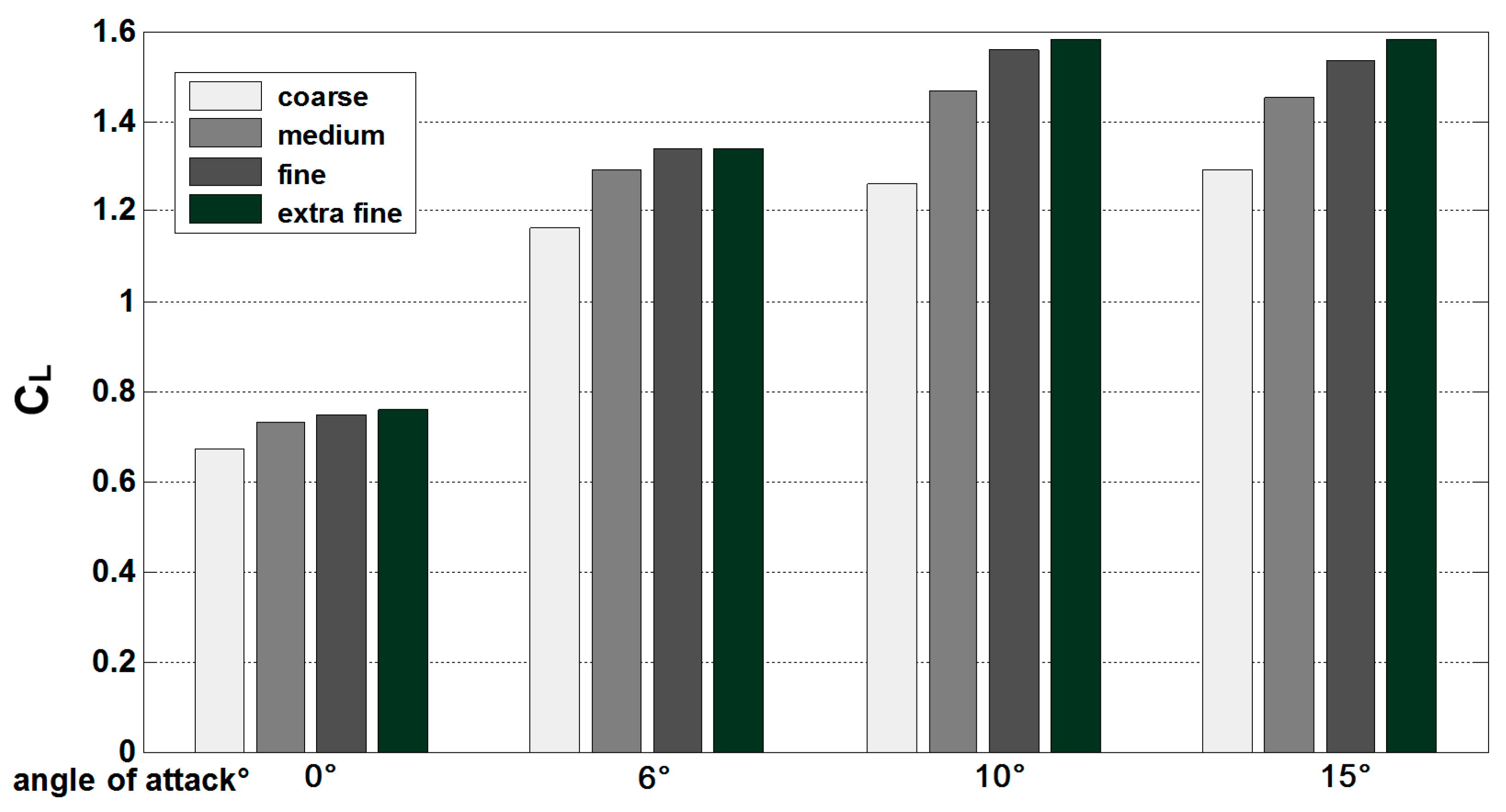
Figure 6.
(a) Lift coefficient and (b) drag coefficient of the elasto-flexible membrane wing, its rigid counterpart and the experiments at Re = 280,000.
Figure 6.
(a) Lift coefficient and (b) drag coefficient of the elasto-flexible membrane wing, its rigid counterpart and the experiments at Re = 280,000.

Figure 7.
(a) Deformed geometry of the elasto-flexible membrane wing for AOA = 12°, 14°, 15°, 16° and 18°; (b) Pressure distribution of the elasto-flexible membrane wing for AOA = 12°, 14°, 15°, 16° and 18°; (c) Geometry of the rigid membrane wing; (d) Pressure distribution of the rigid geometry for AOA = 13°, 14° and 15°.

Figure 8.
(a) Deformed geometry of the elasto-flexible membrane wing for AOA = 6°; (b) Pressure distribution of the elasto-flexible membrane wing for AOA = 6°; (c) Deformed geometry of the elasto-flexible membrane wing for AOA = 15°; (d) Pressure distribution of the elasto-flexible membrane wing for AOA = 15°.
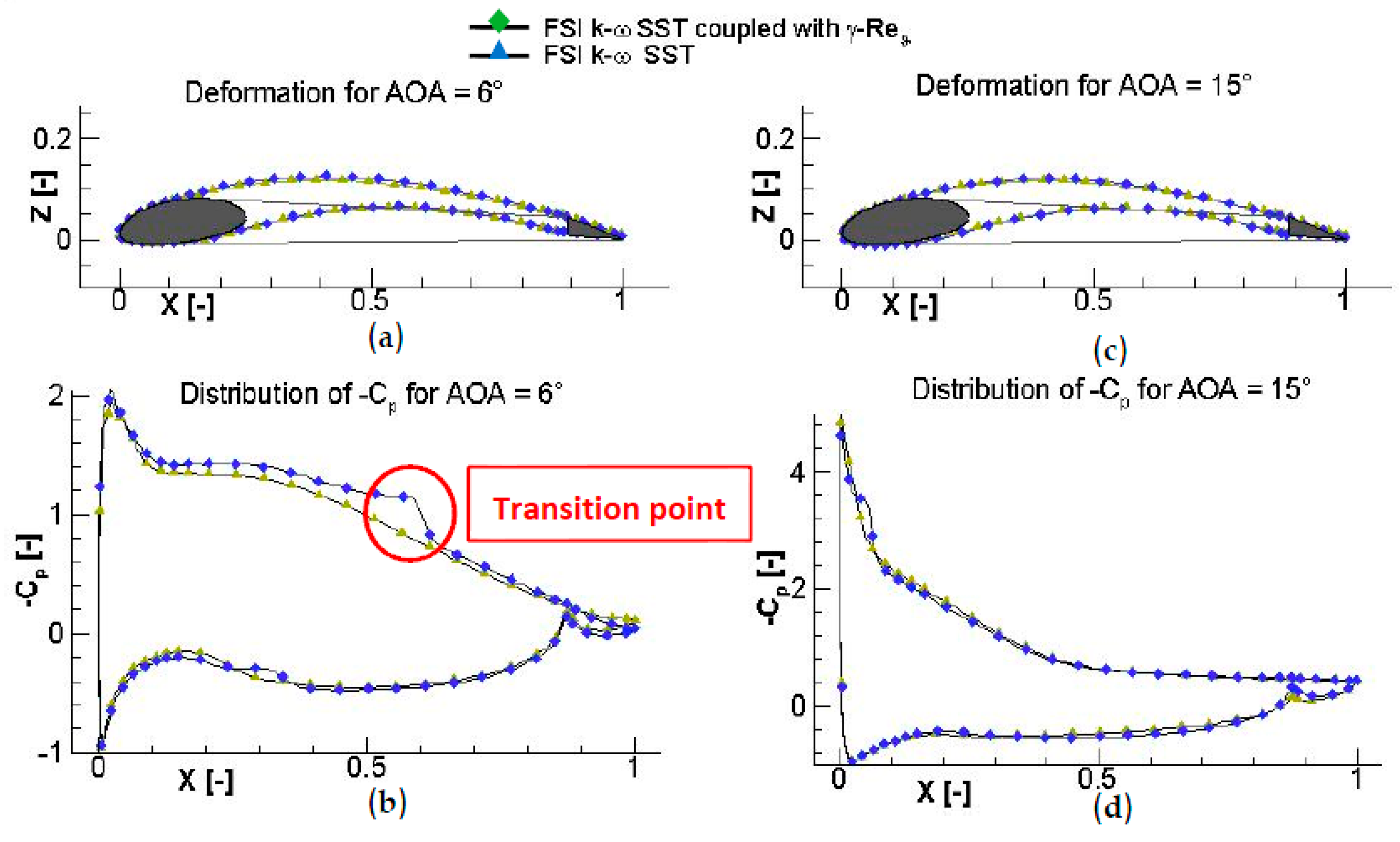
Figure 9.
Turbulence intensity Tu [-] for AOA = 0° (a,b), 6° (c,d) and 15° (e,f) for the k-ω SST model without (left) and with transition (right).
Figure 9.
Turbulence intensity Tu [-] for AOA = 0° (a,b), 6° (c,d) and 15° (e,f) for the k-ω SST model without (left) and with transition (right).
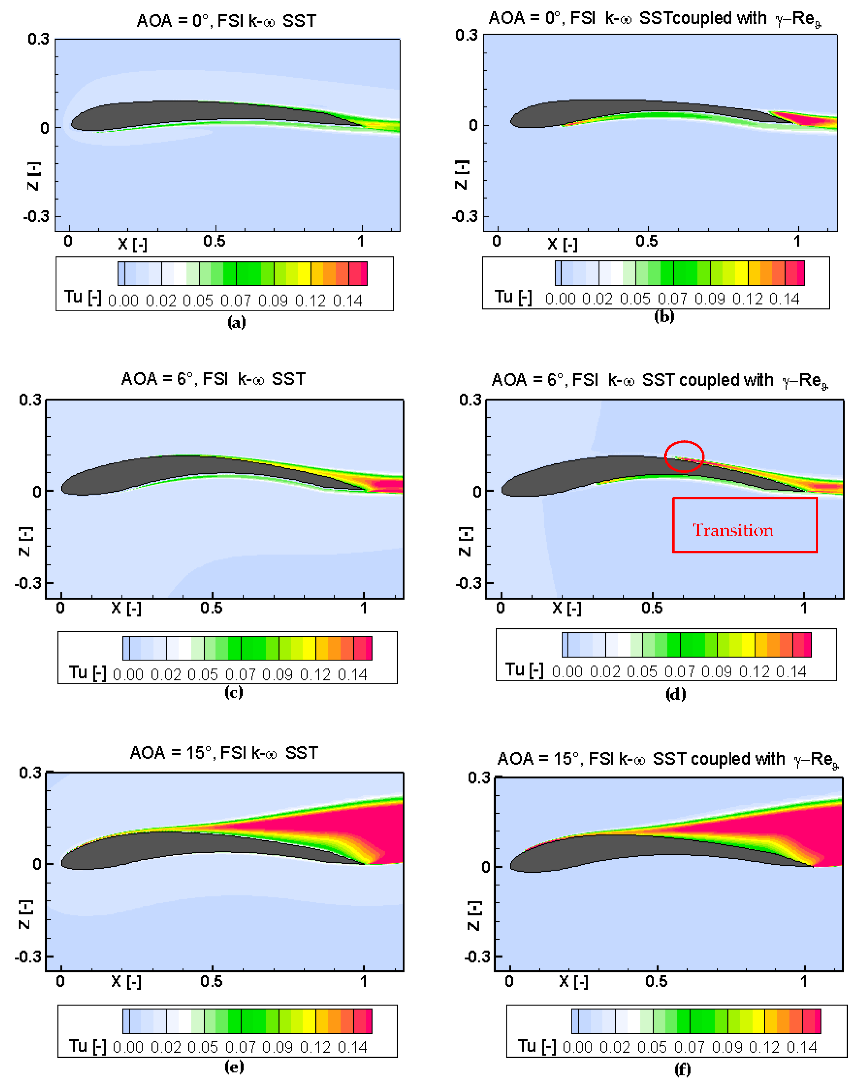
Figure 10.
Deformation of the membrane for the different cases at AOA of 0° (a), 6° (b), 10° (c) and 15° (d) at U∞ = 20 m/s. The experimental tests and the FSI simulations are shown.
Figure 10.
Deformation of the membrane for the different cases at AOA of 0° (a), 6° (b), 10° (c) and 15° (d) at U∞ = 20 m/s. The experimental tests and the FSI simulations are shown.

Figure 11.
Downwash angle β measurement using a hot wire anemometry system for AOA = 6° at Re = 280,000 at 220 mm behind the trailing edge.
Figure 11.
Downwash angle β measurement using a hot wire anemometry system for AOA = 6° at Re = 280,000 at 220 mm behind the trailing edge.

Figure 12.
U and W velocities obtained in (a) for the experiment simulations and in (b) for the FSI simulations at AOA = 6° and U∞ = 20 m/s.
Figure 12.
U and W velocities obtained in (a) for the experiment simulations and in (b) for the FSI simulations at AOA = 6° and U∞ = 20 m/s.

Figure 13.
U and W velocities obtained in (a) for the experiment simulations and in (b) for the FSI simulations at AOA = 15° and U∞ = 20 m/s.
Figure 13.
U and W velocities obtained in (a) for the experiment simulations and in (b) for the FSI simulations at AOA = 15° and U∞ = 20 m/s.


Table 1.
Flow conditions of experimental investigation.
| Measurement Techniques | Flow Conditions | |||
|---|---|---|---|---|
| U∞ [m/s] | q∞ [Pa] | Re | α [°] | |
| Force measurement | 20 | 230 | 280,000 | 0, 2, 4, 6, 8, 10, 12, 14, 15, 16, 17, 18 |
| Hot-wire anemometry | 20 | 230 | 280,000 | 6, 15 |
| Stereo-photogrammetry | 20 | 230 | 280,000 | 0, 6, 10, 15 |
Table 2.
Characteristics of the different tested grids.
| Parameters | Coarse | Medium | Fine | Extra Fine |
|---|---|---|---|---|
| Total nodes number | 39,226 | 80,374 | 159,774 | 299,824 |
| Normal layer | 62 | 90 | 120 | 175 |
| Circumferential layer | 2 × 75 | 2 × 100 | 2 × 140 | 2 × 185 |
| Minimal angle | 26.4 | 26.8 | 27.3 | 27.6 |
| Aspect ratio | 5840 | 3180 | 1930 | 1400 |
© 2017 by the authors. Licensee MDPI, Basel, Switzerland. This article is an open access article distributed under the terms and conditions of the Creative Commons Attribution (CC BY) license (http://creativecommons.org/licenses/by/4.0/).
Share and Cite
MDPI and ACS Style
Piquee, J.; Breitsamter, C. Numerical and Experimental Investigations of an Elasto-Flexible Membrane Wing at a Reynolds Number of 280,000. Aerospace 2017, 4, 39. https://doi.org/10.3390/aerospace4030039
AMA Style
Piquee J, Breitsamter C. Numerical and Experimental Investigations of an Elasto-Flexible Membrane Wing at a Reynolds Number of 280,000. Aerospace. 2017; 4(3):39. https://doi.org/10.3390/aerospace4030039
Chicago/Turabian StylePiquee, Julie, and Christian Breitsamter. 2017. "Numerical and Experimental Investigations of an Elasto-Flexible Membrane Wing at a Reynolds Number of 280,000" Aerospace 4, no. 3: 39. https://doi.org/10.3390/aerospace4030039
Note that from the first issue of 2016, this journal uses article numbers instead of page numbers. See further details here.