Vibratory Reliability Analysis of an Aircraft’s Wing via Fluid–Structure Interactions

1
Laboratoire d’Ingénierie, Management Industriel et Innovation, Faculté des Sciences et Techniques de Settat, Route de Casablanca, 577 Settat, Morocco
2
Laboratoire de Mécanique de Normandie, Institut National des Sciences Appliquées de Rouen, Avenue de l’Université, 76801 Saint Etienne de Rouvray, France
*
Author to whom correspondence should be addressed.
Aerospace 2017, 4(3), 40; https://doi.org/10.3390/aerospace4030040
Submission received: 27 June 2017
/
Revised: 27 July 2017
/
Accepted: 28 July 2017
/
Published: 1 August 2017
Abstract
:The numerical simulation of multiphysics problems has grown steadily in recent years. This development is due to both the permanent increase of IT resources and the considerable progress made in modeling, mathematical and numerical analysis of many problems in fluid and solid mechanics. The phenomena related to fluid/structure mechanical coupling occurs in many industrial situations, and the influence it may have on the dynamic behavior of mechanical systems is often significant. In this paper, a numerical vibratory study is conducted on a three-dimensional aircraft’s wing subjected to aerodynamic loads. Finite volume method (FVM) is used for the discretization of the fluid problem, and finite element method (FEM) is used for the structure’s approximation. In this context, a deterministic model has been proposed in our study, then stochastic analysis has been developed to deal with the statistical nature of fluid–structure interaction parameters. Moreover, probabilistic-based reliability analysis intends to find safe and cost-effective projects.
1. Introduction
The phenomena related to fluid–structure mechanical coupling appear—in various degrees of importance—for any structure in contact with a fluid. The mechanical fluid–structure interaction (FSI) is a problem in which the solid and fluid environments exchange mechanical energy at the interface between them and in both directions such that the fluid exerts forces on the moving structure, which changes its dynamics, and the structure imposes displacements in the fluid and thus changes the characteristics of the fluid flow [1,2].
Physical processes governing such exchanges vary according to the coupling situations, depending on whether or not the fluid is flowing. In the case where the fluid is stagnant, it is a matter of describing small movements of the fluid and the structure around a state of equilibrium at rest. Under these conditions, a description for the dynamics of the interaction in the frequency domain is adapted and generally leads to solving linear problems [3,4].
In the case of a flowing fluid, it is necessary to describe the large motion of fluid and/or structure, and a description of the interaction in the temporal domain is adopted. In this case, the equations describing fluid and structure behavior generally leads to the resolution of nonlinear problems.
The situation is less complicated in a classical problem of a single field (e.g., the case of only one structure or one fluid problem), because in FSI problems we have to simultaneously satisfy boundary conditions, a set of differential equations related to both fluid and structure fields, and a set of physically essential compatibility conditions related to the fluid–structure interface.
On the other hand, one of the main hypotheses in the study of mechanical systems is that the model is deterministic, which means that the parameters used in the model are assumed to be known exactly. However, experimental works show the limitations of such an assumption. This is because there are always differences between calculated and measured quantities, due mainly to the uncertainties in geometry, material properties, boundary conditions, and loads, which can have a considerable impact on the vibrating behaviour of mechanical systems. In order to account for those uncertainties, design procedures based on purely deterministic analyses have been replaced by stochastic and reliability analyses which consider the uncertainties affecting the design parameters for an optimal and robust structural design. These methods make it possible to study the reliability of the components on one hand, and on the other hand the influence of variability of the parameters on the component’s behavior. The mechanical models are often complex, and this complexity should be taken into account by the methods of reliability-mechanical coupling that require a call to the deterministic computation of the mechanical model for repeated sampling of random variables. The number of calls generally increases with the number of random variables, and the time of the calculation becomes prohibitive using traditional methods [5,6]. In the case of this problem, better control of these parameters is thus based on the use of stochastic methods whose main objective is to improve the quality and the reinterpretation of results from simulations.
This paper aims to analyze a 3D aircraft’s wing subjected to aerodynamic loads in order to determine its realistic response due to the exchanged boundary informations. ANSYS is used for creating the volume mesh and the whole computational domain. Two simulation codes based on the finite element method (ANSYS/Mechanical) and the finite volume method (ANSYS/Fluent) were coupled to obtain numerical solutions for the integral equations which determine the airflow pressures, the wing eigenfrequencies, and its respective mode shapes [7,8]. Then, a numerical stochastic method of coupled fluid–structure model and reliability analysis based on the first and the second order reliability methods (FORM and SORM) is applied for analyzing the effect of uncertainties on the numerical results and to find the best compromise between cost and safety in order to supply guidelines for carrying out reliable and cost-effective projects, accounting for the statistical variability of the design parameters.
The following sections discuss the general ideas about these topics. The results demonstrate the applicability, accuracy and efficiency of the proposed methodologies for complex multiphysics problems.
2. Fluid–Structure Interaction (FSI) Problem
2.1. FSI Basic Equations
We present the FSI problems in a domain consisting of a fluid part and a solid part with respective boundaries and and a fluid–structure interface .
The Eulerian formulation is usually employed for the description of fluid flows, because we are usually interested in the properties of the flow at certain locations in the flow domain. The Navier–Stokes equations of incompressible flows may be written on the fluid domain as [1]:
where is the fluid density, v the velocity, f the external force, and the stress tensor, defined as:
Here p is the pressure, I is the identity tensor, is the dynamic viscosity, and is the strain-rate tensor, given by:
The boundary conditions associated to the fluid domain are:
where can be a known velocity profile at the boundary
Most commonly, the structure is described using a Lagrangian description, where the material derivative becomes a partial derivative with respect to time. The structure domain is defined by the Navier equation for a homogeneous and isotropic elastic structure without body force as [1]:
where is the structure density, u the displacement, and the stress tensor.
The structural boundary conditions are the following:
where is the boundary where the displacements are imposed and is the boundary where the forces are imposed.
The stress–strain relation is given by the generalized Hooke’s law:
with the stress vector, S the strain vector, and D the tensor of elastic constants. In the case of a structure consisting of a homogeneous and isotropic material, D is computed from the coefficient of Lamé and , depending on the Young’s modulus E and Poisson’s ratio .
The FSI problem requires the characterization of additional boundary conditions that describe the interface between the fluid and the solid. Dynamic and kinematic conditions represent the essential ones. The force equilibrium requires the stress vectors to be equal as:
Additionally, the normal velocities at the interface have to match as:
2.2. Numerical Discretization
2.2.1. Finite Element Discretization
The discretization by the finite element method requires the use of a weak formulation. To do this, we multiply Equation (6) by a virtual displacement field and integrate the equation on the structure domain [9].
The second member can be written as:
The resulting equation is discretised on each element of domain and border :
The quantities are defined at the nodes of elements using the shape functions , such as:
The scalar product of two vectors is also written . It is the same for the contracted product of two tensors , which is written . Equation (15) becomes:
with the elementary mass matrices, the linear part of the stiffness, the non-linear part of the stiffness, and the vector of external forces:
with:
The system is constructed by assembling the equations of the different elements. We thus arrive, eliminating the trivial solution in the equation of the form:
This system requires special methods of resolution because of the nonlinearity of stiffness, and the resolution requires the calculation of integrals present in the mass and stiffness matrices with achieving time advancement of the problem accounting for the non-linearity.
2.2.2. Finite Volume Discretization
ANSYS/Fluent allows solving the Navier–Stokes equations by a finite volume method. This method consists of integrating Equations (1) and (2) on a control volume (CV). The control volume is centered on a grid node. These boundaries are median portions taken between the boundary elements and their center points (Figure 1) [10].
According to ANSYS/Fluent, the transient term is discretized by Euler’s second order implicit method using a backward formulation, which involves the terms of the current and previous time step. This gives the following equation for the discretization of the transient term:
with the time step. This scheme is conservative in time, implicit, and robust. Moreover, the time step is not limited by the stability of the scheme. Once the different equations are discretized, we can make the assembly of the system of equations. We then obtain a linear matrix system such as:
with the vector of unknowns, including the three components of the velocity vector and pressure:
and the coefficients matrix.
The resolution of this system is possible by using either a decoupled approach or a coupled approach. The solver used in this study is based on a coupled resolution of the previous system. This approach is expected to be faster, but requires the storage of a larger number of variables in memory.
To account for the deformation of the mesh, we use an ALE (arbitrary Lagrangian Eulerian) formulation of the Navier–Stokes equations, discretized on a control volume with volume and boundary , in order to combine the advantages of the Lagrangian and Eulerian formulations, as they are usually exploited for individual structural and fluid mechanics approaches, respectively. The principal idea of the ALE approach is that an observer is neither located at a fixed position in space nor does it move with the material point, but can move “arbitrarily”. Mathematically, this can be expressed by employing a relative velocity in the convective terms of the conservation equations:
ALE formulation brings up the mesh velocity vector with which S moves due to displacements of solid parts in the problem domain. Note that with and the pure Euler and Lagrange formulations are recovered, respectively. The transitional term accounts for the change in the volume of CV, while the advection accounts for advective transport through the CV mobile border [1].
The method for moving the grid in the fluid domain constitutes an important component of the coupled solution procedure, in particular in the case of larger structural deformations. Besides the requirements that no grid folding occurs and that the mesh exactly fits the moving boundaries, one has to take care that distortions of control volumes are kept to a minimum in order to avoid deterioration of the discretization accuracy and the efficiency of the solver. The update of the volume mesh is handled automatically by ANSYS/Fluent at each time step based on the new positions of the boundaries. ANSYS/Fluent allows us to describe the motion using either boundary profiles, user-defined functions (UDFs), or the six degree of freedom solver (6DOF) [10]. Remeshing methods are available in ANSYS/Fluent to update the volume mesh in the deforming regions subject to the motion defined at the boundaries with agglomerating cells that violate the skewness or size criteria, and locally remeshes the agglomerated cells or faces. If the new cells or faces satisfy the skewness criterion, the mesh is locally updated with the new cells (with the solution interpolated from the old cells).
2.3. Fluid–Structure Coupling
The key point of a coupled fluid–structure computation lies in the resolution of the numerical coupling between fluid and structure solvers who should be compatible with the modeling of the physical mechanisms responsible for the coupling between the two systems. As such, it is common to distinguish different types of numerical schemes that induce more or less strong coupling procedures.
The most basic procedure consists of a partitioned coupling with an exchange between fluid and structure solvers alternately in each instance at boundary conditions. This technique has the advantage of being easy from the standpoint of its implementation, since the choice of independent fluid and structure solvers can be free. In a partitioned coupling, the fluid and structure computations are resolved consecutively. It is therefore necessary to predict the displacement of the structure between times and so that the fluid solver can be resolved on an updated domain at each time step and vice versa; the prediction of fluid loadings must be chosen such that the structure solver provides an evaluation of the motion of the consistent interface with respect to the generated loads [11].
Conversely, a monolithic coupling procedure allows the resolution of all the fluid and structure problem unknowns to be considered simultaneously at the same instances. In this case, insurance of convergence to the solution is optimal, but the difficulties of such monolithic approaches are of a different order: the complete system can be difficult to solve, and many structural changes must be made at the level of fluid and structure solvers, loss of software modularity, limitations with respect to the application of different sophisticated solvers in the different fields, and challenges with respect to the problem size and conditioning of the overall system matrix. Hence, they are generally considered not very well suited for application to real-world problems, where often not only specific solution approaches but also specific codes should be used in the single fields. So, we used a partitioned coupling for these reasons.
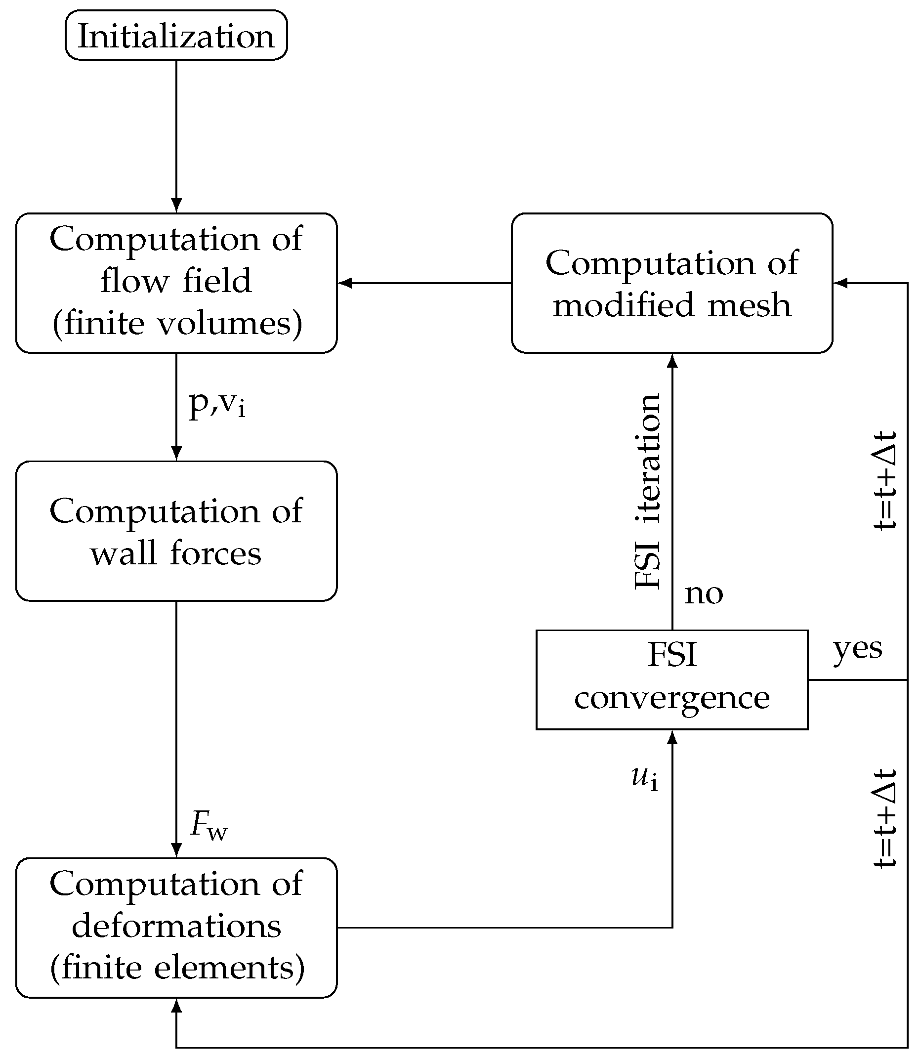
The iteration process in a schematic view for each time step is given in Figure 2. Succeeding the initializations, a determination of the flow field in the defined flow geometry is done. From this, the computed friction and pressure forces on the interacting walls are passed to the structural solver as boundary conditions. So, the fluid mesh is modified due to structural solver computed deformations before the flow solver is started again [1].
The FSI iteration loop is repeated until a convergence criterion is reached, which is defined by the change of the mean displacements:
where m is the FSI iteration counter, N is the number of interface nodes, and denotes the infinite norm [1].
3. Reliability Analysis
Since the material parameters are considered as random variables, the satisfactory performance of a system cannot be absolutely guaranteed. However, it can be expressed in terms of the probability of a certain failure criterion being satisfied.
Reliability is defined as the probability related to a perfect operation of a system (within the bounds specified by the design) during a predefined period in normal operation conditions. Defining the design variables of the structure and a performance function expressed or limit state function as which delimits the surface of failure (defined by the condition ), the safe region and unsafe region of the design space in which the failure occurs, the failure probability is calculated:
where is the joint probability density function (PDF) of the design variables.
In practice, it is impossible to obtain the joint PDF in Equation (27) because of scarcity of statistical data. Even in the case where statistical information is sufficient to determine these functions, it is often impractical to numerically perform the integration indicated in Equation (27). Moreover, the number of random variables is high; these variables may not appear explicitly in the performance function, and there may be correlation among the design variables. These difficulties have motivated the development of various approximate reliability methods. The main approaches to solving this equation are direct integration of PDF over the failure domain, and analytical approximations such as the FORM and SORM, respectively. These methods can be considered as gradient-based methods, since they demand the evaluation of the partial derivatives of the limit state function with respect to the random variables at each iteration step.
In reliability analysis, which involves random variables , the deterministic optimal solution is not considered to be the exact solution of the optimum design, but is one of the most probable designs. In this case, the failure surface or limit state function is given by This surface defines the limit between the safe region and unsafe region of the design space. The failure occurs when , and the failure probability is calculated as
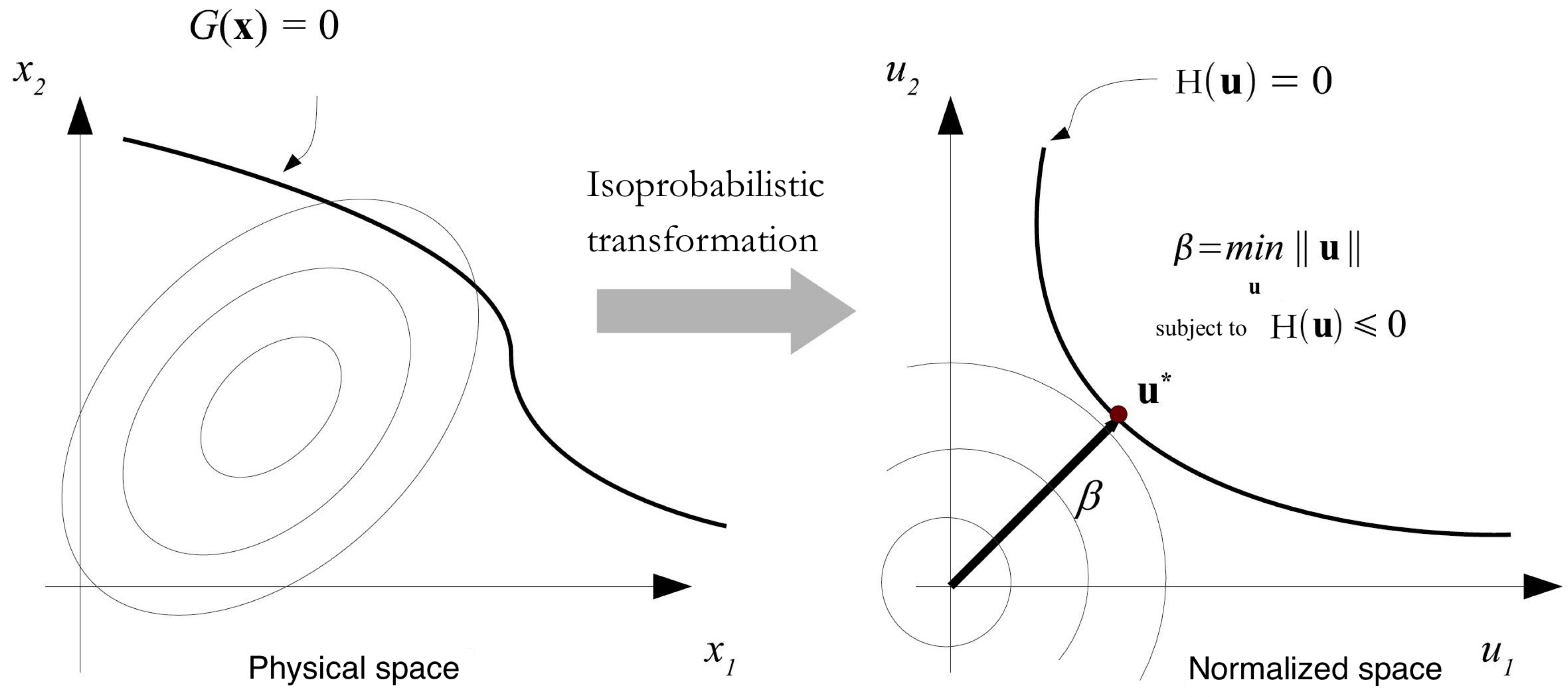
The reliability index is introduced as a measure of the reliability level of the system, and is estimated in the so-called reduced coordinate system, where the random variables are statistically independent with zero mean and unit standard deviation.
Thus, a pseudo-probabilistic transformation must be defined for mapping the original space into the reduced coordinate system. Considering that the probability density in the reduced space decays exponentially with the distance from the origin of this space, the point with maximum probability of failure on the limit state surface, called the most probable point (MPP), is the point of minimum distance from the origin. The reliability index is thus defined as the minimum distance between the origin of the reduced space and the hyper surface representing the limit state function (see Figure 3). Hence, it is possible to find the MPP or design point by solving a constrained optimization problem that is [6,12,13]:
where is the distance in the normalized random space.
By formally introducing a cumulative density function of the normal probability distribution function, the first-order approximation (tangent plane at the MPP) to can be written as [14]:
This corresponds to the substitution of the hyper surface by the hyper plane passing through the point defined by .
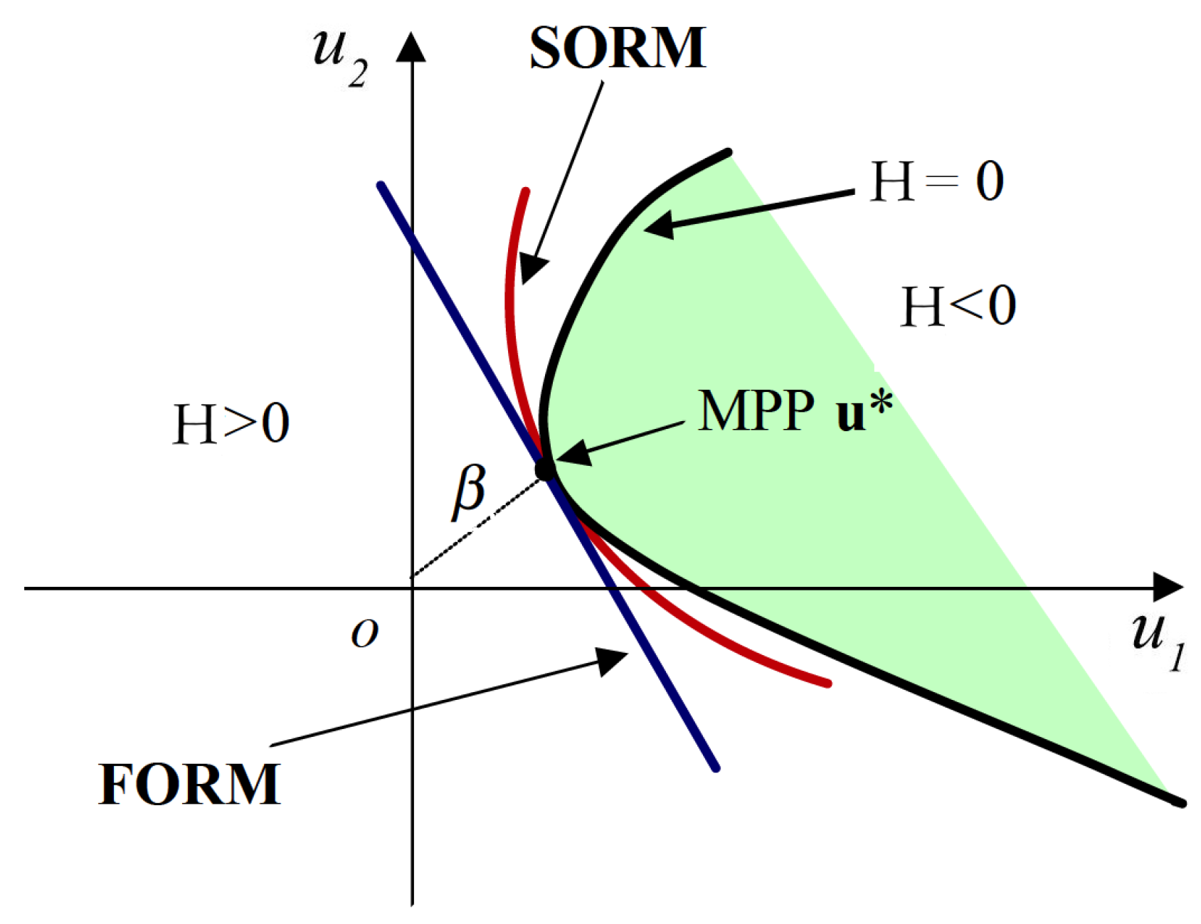
In this paper, the proposed reliability analysis methods employed to compute the probabilities of failure are FORM and SORM. FORM is based on linear approximation of the limit state surface tangent to the MPP of the failure surface to the origin of a reduced coordinate system. Thus, the random variables are transformed to reduced variables in a reduced coordinate system. SORM estimates the probability of failure by using a nonlinear approximation of the limit state function by a second-order representation (see Figure 4). The curvatures of the limit state function are approximated by the second-order derivatives with respect to the original variables. Thus, SORM improves FORM by including additional information about the curvature of the limit state function through a curvature parameter. It is important to note that the MPP of FORM and SORM is the same. Additionally, SORM uses the reliability index value estimated through FORM as initial value.
4. Numerical Simulations
FSI two-way coupling analysis can be carried out in ANSYS Workbench by doing a connection between the coupling participants and a component system called System Coupling [15], which either sends or receives data from the two coupling participants (ANSYS/Fluent and ANSYS/Mechanical) [16]. The evaluation of convergence is done at the end of every coupling iteration [17]. However, for the one-way coupling, thefluid solver does not receive the boundary displacement from the mechanical application, and the loads can be linked directly between the two systems.
First, ANSYS/Fluent transfers the pre-requested fluid loads to ANSYS/Mechanical to get nodal displacements. The convergence condition is then collected for the system coupling from the two solvers and starts the next time step. The computed solution of ANSYS/Mechanical is given back to ANSYS/Fluent to resolve a new set of fluid loads due to nodal displacements of the previous step. Reaching the convergence criterion of data transfer defines the end of this continuous coupling iteration.
Initially, ANSYS is used to create the geometric models with appropriate dimensions. The wing’s cross-sectional area is defined to be a straight line and a spline, and it has uniform configuration along its length. The wing hangs freely on one end and is held fixed to the body at the other. The objective in this section is to determine the eigenfrequencies of the wing undergoing airflow in order to represent the effect of aerodynamic loads on the wing.
Hybrid-unstructured mesh was generated with 518,762 cells and 99,000 nodes points for CFD computations. It also contains mixtures of tetrahedral, pyramidal , and prism cells in the boundary layer region. The structure dynamics finite element mesh of the wing has a total number of 5991 node points and 1120 elements. The use of dynamic mesh in the current version of ANSYS/Fluent is not compatible with hexahedral cells; this is why the unstructured volume CFD mesh is constructed with tetrahedral cells. Figure 5 shows the mesh of the whole computational fluid and structural domains with the adequate boundary conditions.
Table 1 representes the material and geometrical properties of the coupled system:
4.1. Finite Volume (FV)/Finite Element (FE) Results
We begin by the validation of our fluid–structure interaction in the deterministic case. In our numerical study, we consider a 3D wing subjected to airflow. This simulation illustrates the methodology proposed in a deterministic analysis.
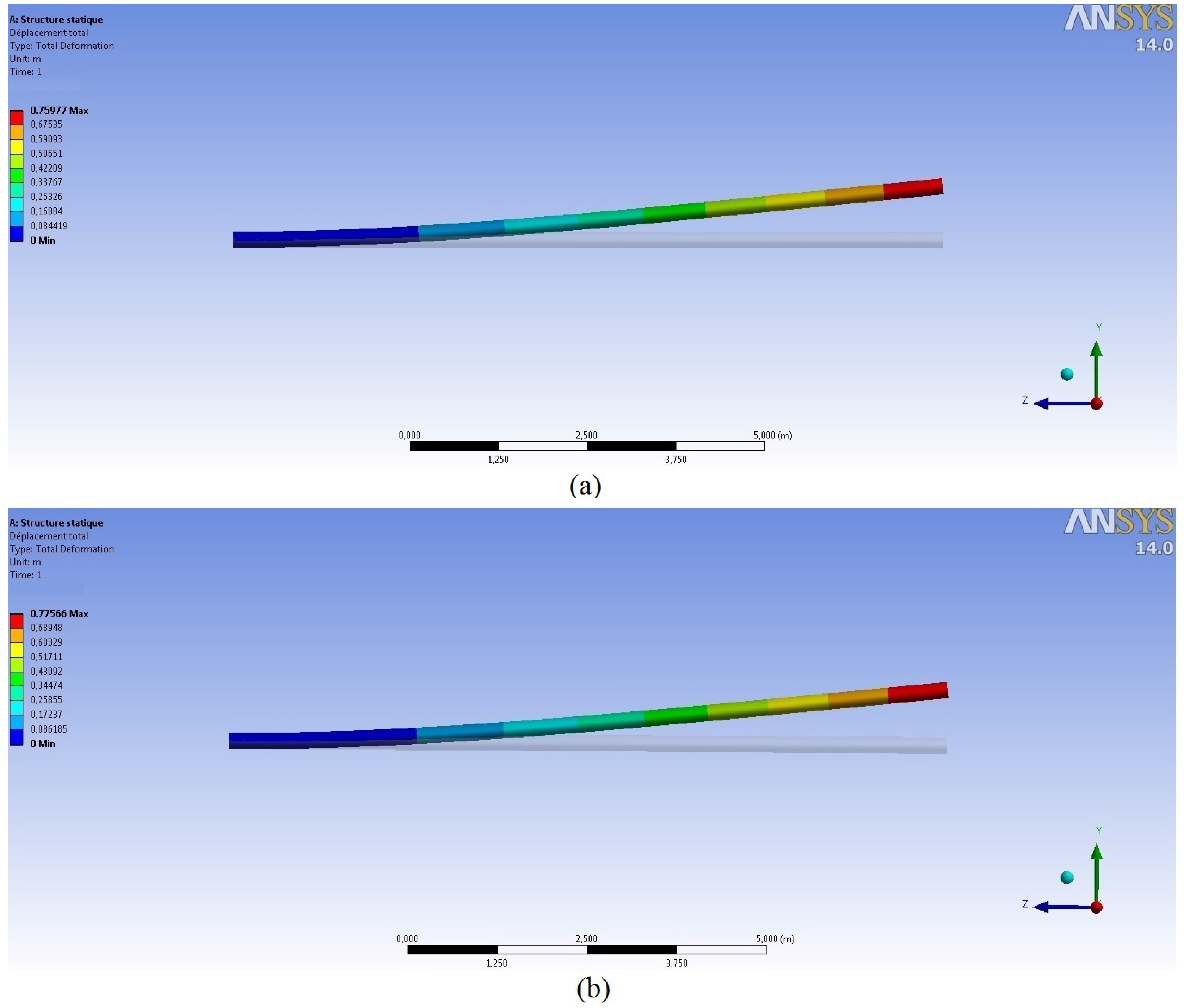
Table 2 and Figure 6 represent the maximum displacement of the wing tip and the total deformation of the wing, respectively, with fluid’s velocity inlet V = 200 m/s, for one-way and two-way coupling:
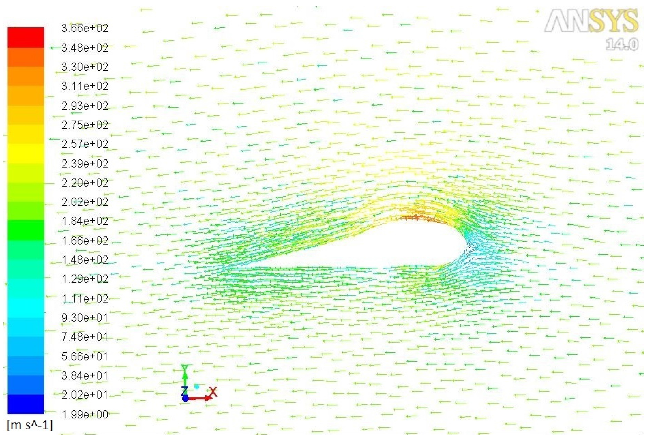
Figure 7 and Figure 8 respectively show the fluid pressure and velocity. The airflow passing under the wing—called the intrados—slowed, and the one passing above—called the extrados—accelerated. So, the pressure under the wing will be greater than the one over it (the blue area in Figure 8). The lift force is then the result of this pressure difference between the intrados and the extrados flow around the wing.
4.2. Prestressed Modal Analysis
4.2.1. Deterministic Study
The form of the eigenvalue and eigenvector problem to be solved for this analysis is:
where and are the structure stiffness matrix and mass matrix, respectively.
4.2.2. Probabilistic Study
The accuracy of the material values under concrete conditions increases the validity of the results of a deterministic analysis. In reality, every form of an analysis model has to deal with significant dispersion. A probabilistic study is used to determine the effect of one or more variables on the analysis outcome. A Monte Carlo simulation method draws samples directly from the probability distributions of the random variables. This procedure is very robust and relatively easy to apply. A sample size of set independent realizations is generally sufficient to obtain a suitable estimate for the mean and variance and to provide information on the basic shape of the distribution. However, Monte Carlo simulation requires a large number of performance evaluations of the random variables in order to estimate the resulting probability distributions.
To simplify, in this paper we have chosen to consider only the sources of uncertainties related to the material properties, and those concerning the other elements of the structure (geometry, boundary conditions, and mechanical behavior) have not been taken into account [18].
Table 4 contains the means of random variables and their standard deviations (SDs) used in this study and the distributions laws chosen.
In this context, the stochastic calculation was carried out using the probabilistic design system of the ANSYS code. This tool is based on a calculation with Monte Carlo simulation (MC) for 100 samples and the response surface method (RSM) for 9 samples.
Table 5 shows the means and standard deviations of the natural frequencies of the wing with airflow.
4.3. Reliability Study
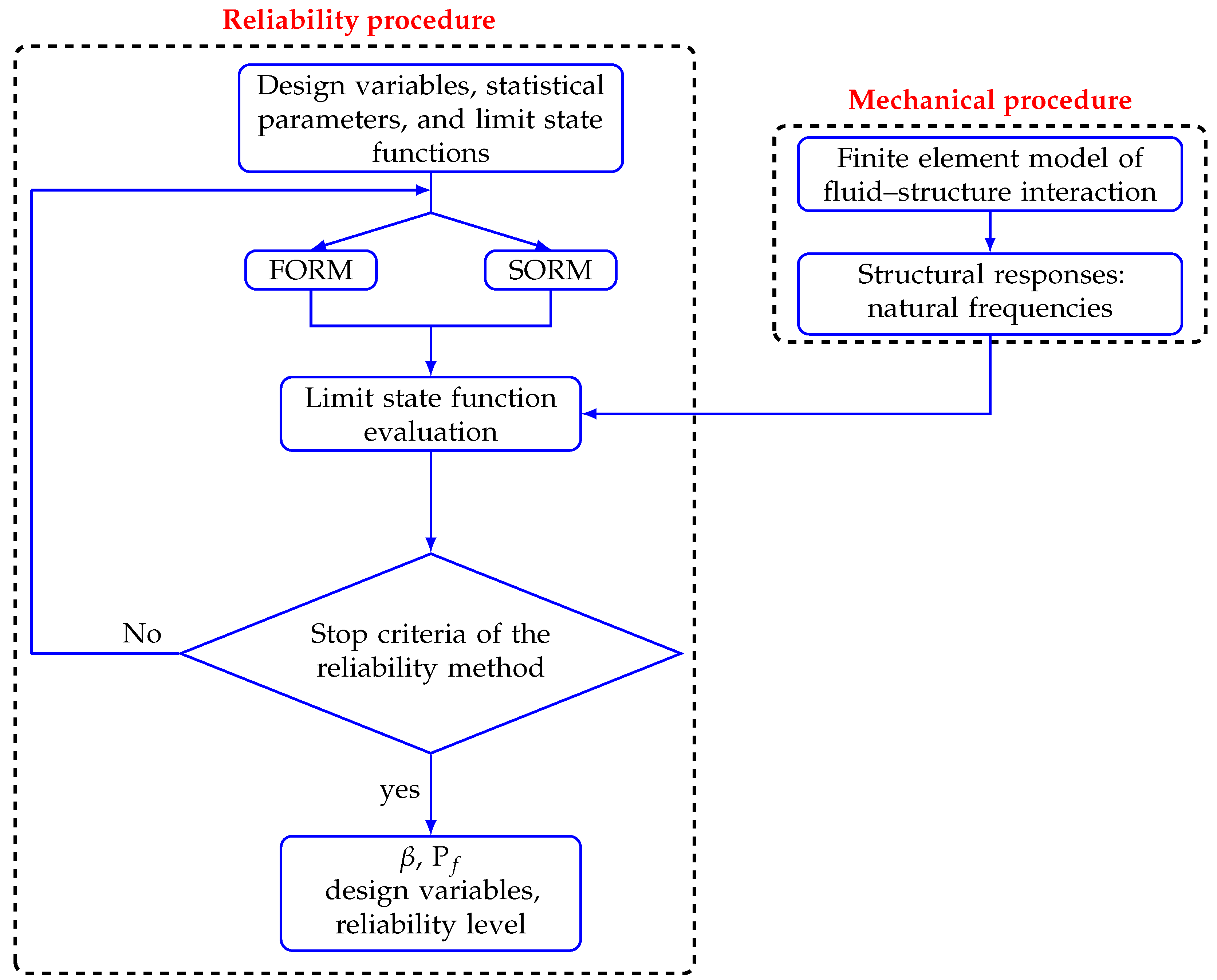
The reliability analysis methodology (shown in Figure 10) used in this numerical simulation integrates a set of reliability analysis tools (based on FORM and SORM) developed under MATLAB with finite element analysis of the fluid–structure interaction problem using this programming environment (for the first numerical application) and using the commercial software ANSYS (for the second numerical application). In the numerical application, the reliability analysis considers the deterministic and stochastic analysis.
The reliability study was based on an implicit limit state function G based on the first natural frequency of the coupled system limited by :
Table 6 illustrates the numerical results obtained from FORM and SORM approaches.
The comparison of results found by the two approaches show small differences between the first- and second-order approximations for the estimation of the reliability index and the probability of failure P Since the approximation of the performance function in SORM is better than that in FORM, SORM is generally more accurate than FORM. However, since SORM requires the second-order derivative, it is not as efficient as FORM when the derivatives are evaluated numerically. If we use the number of performance function evaluations to measure the efficiency, SORM needs more function evaluations and more computer time than FORM.
5. Conclusions
In this paper, a numerical vibratory study is conducted on a three-dimensional aircraft’s wing subjected to airflow, and deterministic, probabilistic, and reliability analyses are proposed for the resolution of fluid–structure interaction problems. The developed methodology integrates finite element and reliability analyses which enable the assessment of the reliability index in coupled fluid–structure systems. The set of reliability tools is based on FORM and SORM methods. Numerical application in dynamics coupled fluid–structures 3D systems—considering material probabilistic variables—were performed in order to check the efficiency and accuracy of the suggested algorithms. Regarding the performance of analysis tools, it can be concluded that the presented methodology is able to handle implicit limit state functions based on numerical models of aircraft’s wing problems. The results obtained are considered satisfactory, and show the potentialities of the procedure methodology for use in complex coupled fluid–structure systems—especially for aeroelastic ones.
Acknowledgments
The authors would like to thank “Erasmus Mundus Programme, Action 2 - STRAND 1, Lot 1, North Africa Countries” for their financial support for the realization of this work.
Author Contributions
Rabii El Maani performed the work, conducted the analyses and wrote the manuscript. Bouchaïb Radi and Abdelkhalak El Hami contributed in reviewing the paper and provided the feedback and advice.
Conflicts of Interest
The authors declare no conflicts of interest.
References
- Souli, M.; Benson, D.J. Arbitrary Lagrangian-Eulerian and Fluid-Structure Interaction; ISTE Ltd. and John Wiley & Sons: New York, NY, USA, 2010. [Google Scholar]
- Zheng, Y.; Yang, H. Coupled fluid structure flutter analysis of a transonic fan. Chin. J. Aeronaut. 2011, 24, 258–264. [Google Scholar] [CrossRef]
- Sigrist, J.F. Interaction Fluide-Structure, Analyse Vibratoire par Éléments Finis; Ellipses: Paris, France, 2011. [Google Scholar]
- El-Maani, R.; Radi, B.; El-Hami, A. Reliability study of a coupled three dimensional system with uncertain parameters. J. Adv. Mater. Res. 2015, 1099, 87–93. [Google Scholar] [CrossRef]
- El-Hami, A.; Radi, B. Uncertainty and Optimization in Structural Mechanics; John Wiley & Sons: London, UK, 2013. [Google Scholar]
- El-Hami, A.; Radi, B. Fiabilité et Optimisation des Systèmes; Ellipses: Paris, France, 2011. [Google Scholar]
- El-Maani, R.; Makhloufi, A.; Radi, B.; El-Hami, A. RBDO analysis of the aircraft wing based aerodynamic behavior. Struct. Eng. Mech. 2017, 61, 441–451. [Google Scholar] [CrossRef]
- Molina-Aiz, F.; Fatnassi, H.; Boulard, T.; Roy, J.; Valera, D. Comparison of finite element and finite volume methods for simulation of natural ventilation in greenhouses. Comput. Electron. Agric. 2010, 72, 69–86. [Google Scholar] [CrossRef]
- Chopra, A. Dynamics of Structures, 2nd ed.; Pearson Prentice Hall: Upper Saddle River, NJ, USA, 2001. [Google Scholar]
- ANSYS. Fluent Theory Guide 14.0; Technical Report; ANSYS: Canonsburg, PA, USA, 2013. [Google Scholar]
- Schafer, M.; Lange, H.; Heck, M. Implicit Partitioned Fluid-Structure Interaction Coupling. In Proceedings of the ASME 2006 Pressure Vessels and Piping/ICPVT-11 Conference, Vancouver, BC, Canada, 23–27 July 2006. [Google Scholar]
- Radi, B.; El-Hami, A. Reliability analysis of the metal forming process. Math. Comput. Model. 2007, 45, 431–439. [Google Scholar] [CrossRef]
- Moro, T.; El-Hami, A.; Moudni, A.E. Reliability analysis of a mechanical contact between deformable solids. Probab. Eng. Mech. 2002, 17, 227–232. [Google Scholar] [CrossRef]
- Haldar, A.; Mahadevan, S. Reliability Assessment Using Stochastic Finite Element Analysis; John Wiley & Sons, Inc.: New York, NY, USA, 2000. [Google Scholar]
- El-Maani, R.; Radi, B.; El-Hami, A. Comparison of the FE/FE and FV/FE treatment of fluid-structure interaction. Int. J. Eng. Res. Appl. 2015, 5, 59–69. [Google Scholar]
- ANSYS. 14.0-User Guide; ANSYS Workbench: Canonsburg, PA, USA, 2013. [Google Scholar]
- Khalid, S.; Zhang, L.; Zhang, X.; Sun, K. Three-dimensional numerical simulation of a vertical axis tidal turbine using the two-way fluid structure interaction approach. J. Zhejiang Univ. Sci. A 2013, 14, 574–582. [Google Scholar] [CrossRef]
- Akramin, M.R.M.; Abdulnaser, A.; Hadi, M.S.A.; Ariffin, A.K.; Mohamed, N.A.N. Probabilistic analysis of linear elastic cracked structures. J. Zhejiang Univ. Sci. A 2007, 8, 1795–1799. [Google Scholar] [CrossRef]
Figure 1.
Control volume for 2D mesh.
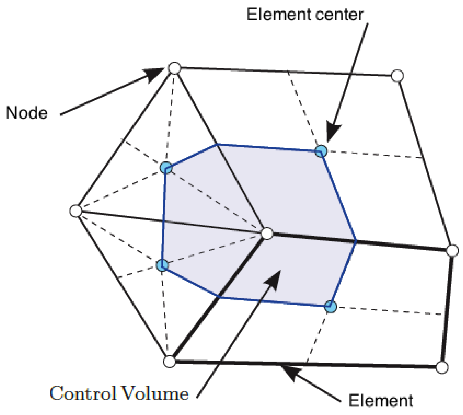
Figure 2.
Coupling procedure. FSI: fluid–structure interaction.

Figure 3.
Transformation between the physical space and the normalized one.

Figure 4.
Comparison of first and second order reliability methods (FORM and SORM). MPP: most probable point.
Figure 4.
Comparison of first and second order reliability methods (FORM and SORM). MPP: most probable point.

Figure 5.
Computational mesh and boundary conditions.
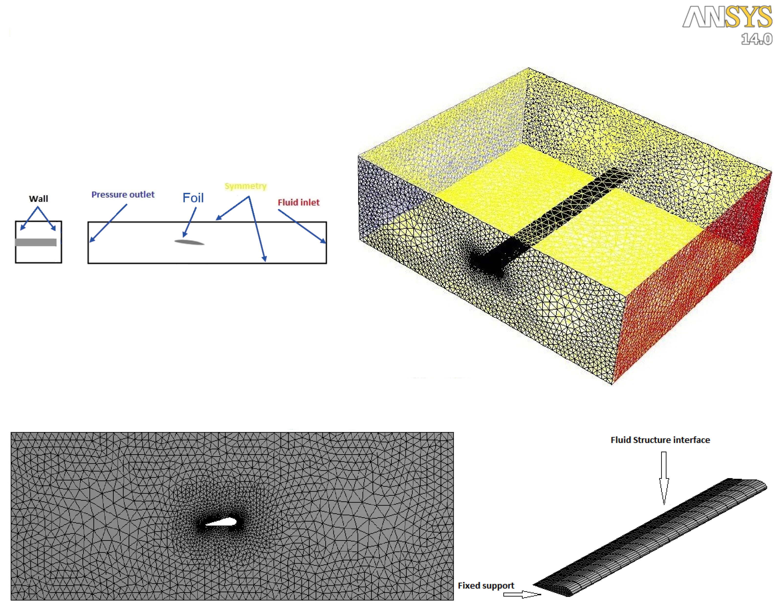
Figure 6.
Total deformation of the wing: (a) one-way coupling; (b) two-way coupling.

Figure 7.
Variation of fluid velocity.

Figure 8.
Variation of fluid pressure.
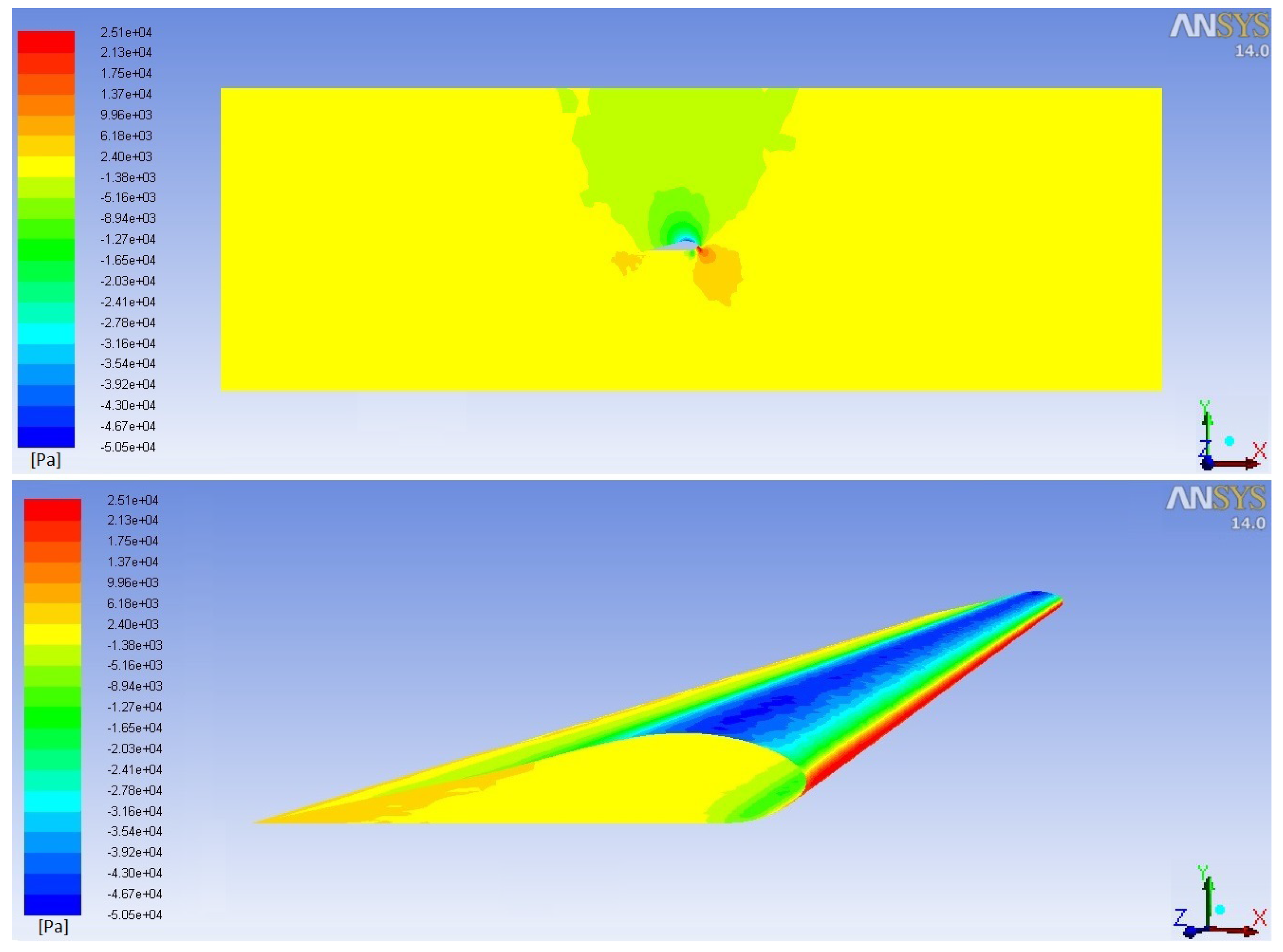
Figure 9.
Mode shapes of the wing.
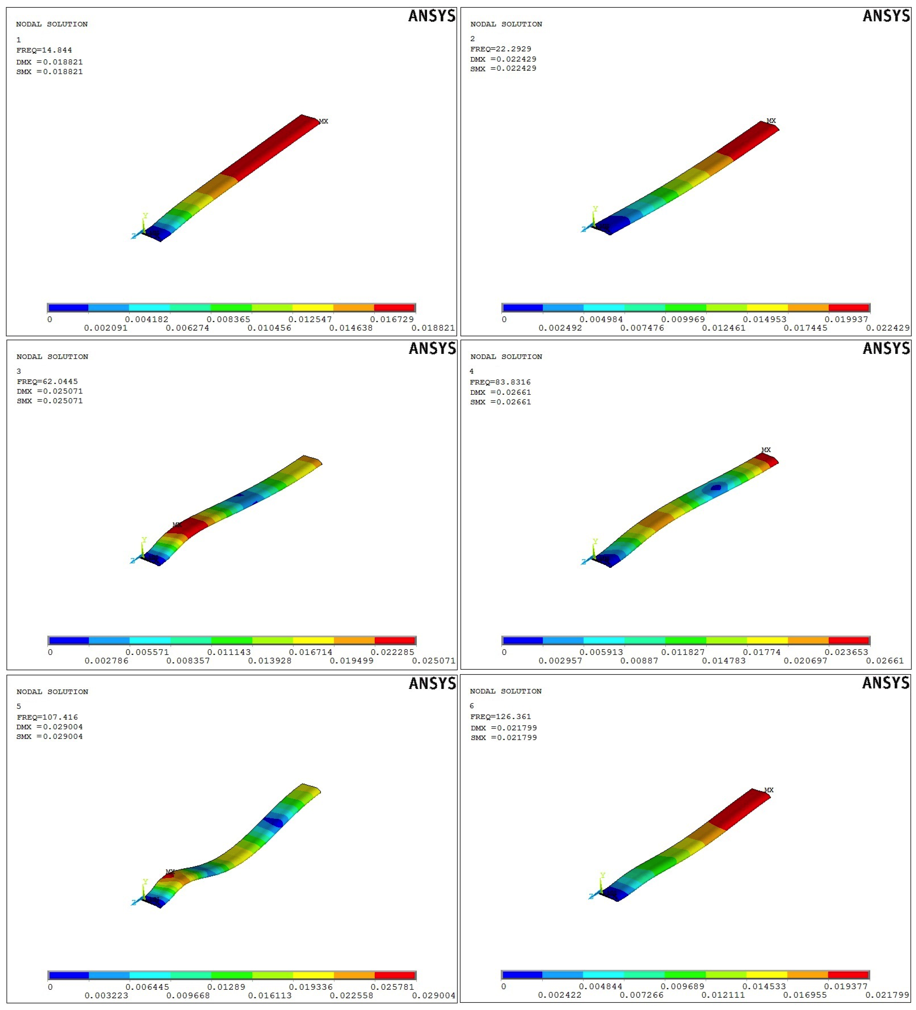
Figure 10.
Reliability analysis methodology.


Table 1.
Material and geometrical properties.
| Structure | Length | L = 10 m |
| Young’s modulus | E = Pa | |
| Structure’s density | = 2770 kg·m | |
| Poisson’s ratio | = | |
| Fluid | Length | L = 12 m |
| Fluid’s density | = kg·m | |
| Viscosity | = kg/(m·s) |
Table 2.
Maximum displacement of the wing.
| Maximum Displacement (m) | |
|---|---|
| One-way | Two-way |
| 0.75977 | 0.77566 |
Table 3.
Natural frequencies of the wing.
| Mode Shapes | Natural Frequencies (Hz) | |
|---|---|---|
| One-Way | Two-Way | |
| 1 | 14.844 | 14.853 |
| 2 | 22.293 | 22.290 |
| 3 | 62.045 | 62.014 |
| 4 | 83.832 | 83.766 |
| 5 | 107.42 | 107.36 |
| 6 | 126.36 | 126.36 |
Table 4.
Moments and distribution laws of the parameters of the problem.
| Parameters | Means | SD | Distribution |
|---|---|---|---|
| Young’s Modulus (Pa) | Gaussian (,) | ||
| Density (kg·m) | 2770 | 83.1 | Gaussian (,) |
Table 5.
Natural frequencies (Hz) of the wing. MC: Monte Carlo; RSM: response surface method; SD: standard deviation.
Table 5.
Natural frequencies (Hz) of the wing. MC: Monte Carlo; RSM: response surface method; SD: standard deviation.
| Modes | Deterministic Case | MC | SD | RSM | SD |
|---|---|---|---|---|---|
| 1 | 14.844 | 14.852 | 0.262 | 14.871 | 0.491 |
| 2 | 22.293 | 22.304 | 0.348 | 22.328 | 0.645 |
| 3 | 62.045 | 62.089 | 1.268 | 62.183 | 2.376 |
| 4 | 83.832 | 83.883 | 1.289 | 83.990 | 2.374 |
| 5 | 107.42 | 107.470 | 2.062 | 107.57 | 3.839 |
| 6 | 126.36 | 126.392 | 3.691 | 126.47 | 6.547 |
Table 6.
Reliability results.
| Parameters | FORM | SORM |
|---|---|---|
| Young’s modulus (Pa) | ||
| Density (kg·m) | 3002.6 | 3002.6 |
| Reliability index | 3.372 | 3.3831 |
| Probability P | 0.00037 | 0.00035 |
| Reliability | 99.963 | 99.964 |
© 2017 by the authors. Licensee MDPI, Basel, Switzerland. This article is an open access article distributed under the terms and conditions of the Creative Commons Attribution (CC BY) license (http://creativecommons.org/licenses/by/4.0/).
Share and Cite
MDPI and ACS Style
El Maani, R.; Radi, B.; El Hami, A. Vibratory Reliability Analysis of an Aircraft’s Wing via Fluid–Structure Interactions. Aerospace 2017, 4, 40. https://doi.org/10.3390/aerospace4030040
AMA Style
El Maani R, Radi B, El Hami A. Vibratory Reliability Analysis of an Aircraft’s Wing via Fluid–Structure Interactions. Aerospace. 2017; 4(3):40. https://doi.org/10.3390/aerospace4030040
Chicago/Turabian StyleEl Maani, Rabii, Bouchaïb Radi, and Abdelkhalak El Hami. 2017. "Vibratory Reliability Analysis of an Aircraft’s Wing via Fluid–Structure Interactions" Aerospace 4, no. 3: 40. https://doi.org/10.3390/aerospace4030040
Note that from the first issue of 2016, this journal uses article numbers instead of page numbers. See further details here.