Discontinuous Galerkin Finite Element Investigation on the Fully-Compressible Navier–Stokes Equations for Microscale Shock-Channels


Centre for Computational Engineering Sciences, Cranfield University, Cranfield, Bedfordshire MK43 0AL, UK
*
Author to whom correspondence should be addressed.
Aerospace 2018, 5(1), 16; https://doi.org/10.3390/aerospace5010016
Submission received: 24 November 2017
/
Revised: 10 January 2018
/
Accepted: 30 January 2018
/
Published: 3 February 2018
(This article belongs to the Special Issue Computational Aerodynamic Modeling of Aerospace Vehicles)
Abstract
:Microfluidics is a multidisciplinary area founding applications in several fields such as the aerospace industry. Microelectromechanical systems (MEMS) are mainly adopted for flow control, micropower generation and for life support and environmental control for space applications. Microflows are modeled relying on both a continuum and molecular approach. In this paper, the compressible Navier–Stokes (CNS) equations have been adopted to solve a two-dimensional unsteady flow for a viscous micro shock-channel problem. In microflows context, as for the most gas dynamics applications, the CNS equations are usually discretized in space using finite volume method (FVM). In the present paper, the PDEs are discretized with the nodal discontinuous Galerkin finite element method (DG–FEM) in order to understand how the method performs at microscale level for compressible flows. Validation is performed through a benchmark test problem for microscale applications. The error norms, order of accuracy and computational cost are investigated in a grid refinement study, showing a good agreement and increasing accuracy with reference data as the mesh is refined. The effects of different explicit Runge–Kutta schemes and of different time step sizes have also been studied. We found that the choice of the temporal scheme does not really affect the accuracy of the numerical results.
1. Introduction
It was 1959 when Richard Feynman gave his famous lecture at the meeting of the American Physical Society at Caltech called “There’s Plenty of Room at the Bottom”, where he proposed two challenges with a prize of $10,000 each: the first one was to design and build a tiny motor, while the second one was to write the entire Encyclopædia Britannica on the head of a pin.
Nowadays, his speech is considered as the foundation of modern nanotechnology, since he highlighted the possibility to encode a number of pieces of information in very small spaces, hence producing small and compact devices [1]. All those extremely small devices having characteristic length of less than 1 mm but more than 1 micron are called microelectromechanical systems (MEMS) and, as the name suggests, they combine both electrical and mechanical components [2]. MEMS are small devices made of miniaturized structures, sensors, actuators and microeletronics and their components are between 1 and 100 micrometers in size. In recent years, several MEMS have been designed and developed, from small sensors to measure pressure, velocity and temperature, to micro-heat engines and micro-heat pumps and their numerical investigations are indispensable.
From a historical point-of-view, a pioneer experimental work on shock wave propagation in a low-pressure small-scale shock-tube was carried out by Duff (1959) [3], where a non-linear attenuation of the shock wave propagation for a certain diaphragm pressure ratio was observed. Other experimental works were performed by Roshko (1960) [4] and Mirels (1963, 1966) [5,6] confirming the strong attenuation of the shock wave and the acceleration of the contact surface, which propagates behind the shock wave in the classic shock-tube test case. The time interval between the shock wave and the contact surface measured at a certain point—which is also known as flow duration—rarefaction effects and thermal creeping were explained in depth. It is important to note that experimental and numerical studies on shock waves in different fields of engineering sciences attracted researchers over the past seventy years [3,4,5,6,7,8,9,10,11,12,13,14]. However, researchers paid particular attention to microscale shock waves and rarefied gas dynamics recently, especially for aerospace applications. This is due to the fact that microengines are used in the development of aerospace propulsion systems, because of their reduced size and achievable high power density. One of the greatest difficulty in the design process of microengines is that the fast heat loss results in low efficiency of these microdevices. Therefore, researchers devoted attention to carrying out experimental and numerical works on shock wave propagation and formation in micro shock-tubes and channels for MEMS applications [15,16,17,18].
In the aerospace industry, microfluidics is becoming more and more popular having applications mainly in aerodynamics, micropropulsion, micropower generation and in life support and environmental control for space applications. For instance, MEMS can be adopted for flow control problems for both free and wall bounded shear layers flows. In 1998, Smith et al. [15] studied experimentally the control of separated flow on unconventional airfoils using synthetic jet actuators to create a “virtual aerodynamic shaping” of the airfoil in order to modify the airfoil characteristics. Microfluidics is also used through fluidic oscillators in order to produce high-frequency perturbations for example to decrease jet-cavity interaction tones [16]. MEMS-based devices are adopted in the aerospace industry for the sake of turbulent boundary layer control. In fact, the small sizes of those systems (high density devices) allow to study near-wall flow structures [17]. In space applications, micropropulsive devices are designed and developed for miniaturized satellites, mainly used for global positioning systems or to serve generic platforms [18]. A detailed review on the application of microfluidics related devices in the aerospace industrial sector can be found in [18].
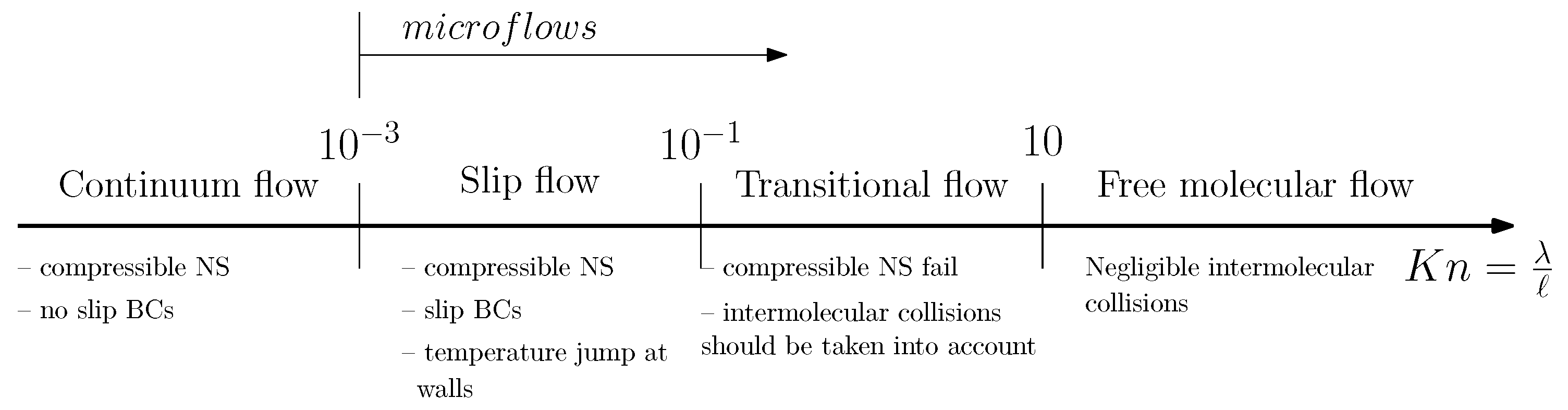
The flow behavior at those microscales is in general characterized by a granular nature for liquids and a rarefied behavior for gases; the walls “move”, hence the classical no slip boundary conditions adopted in the macro regime fails. In agreement with [19], it is possible to classify the main differences among macrofluidics and microfluidics in the following list: noncontinuum effects, surface-dominated effects, low Reynolds number effects and multiscale and multiphysics effects. Furthermore, it is also observed that the diffusivity effects play an important role at this scales (see, e.g., [20]), especially when compared with the transport effects of the flow. Dealing with gases in micro devices, it is common practice to classify different flow regimes through the dimensionless Knudsen number . Let be the mean-free path , which is the average distance traveled by a molecule between two consecutive collisions; denoting with ℓ the characteristic length of the generic problem considered (e.g., the hydraulic diameter for a channel flow problem), the Knudsen number is defined as .
Microfluidics can be modeled with two different approaches. The first one is the continuum model, and the flow is considered as a continuous and indivisible matter, while in the molecular model, the fluid is seen as a set of discrete particles. These models are valid in specific flow regimes determined by the Knudsen number and, when increases, the validity of the continuum approach becomes questionable and the molecular approach should be adopted, as briefly sketched in Figure 1.
When the continuum approach is adopted, the fully-compressible Navier–Stokes (CNS) equations must be numerically solved. In the literature, this is usually performed adopting finite volume solvers. In the present work, the authors investigate how the discontinuous Galerkin finite element method (DG–FEM) performs applied to compressible flows at microscale levels in the slip flow regime (low Knudsen number). This method is selected because it takes advantages from the classical finite element method (FEM) and the finite volume method (FVM) since discontinuous polynomial functions are used and a numerical flux is defined among cells to reconstruct the solution. To verify the DG–FEM code, due to a lack of experimental data in microfluidics, the Zeitoun’s test case [21] is adopted, which consists of a mini viscous shock channel problem numerically solved. In particular, they adopted the following models: the CNS equations in a FVM context, DSMC (Direct Simulation Monte Carlo) for the Boltzmann equation and the kinetic model BGKS (Bhatnagar–Gross–Krook with Shakhov equilibrium distribution function) model. In our work, the open source MATLAB code—developed by Hesthaven and Warburton [22]—has been adopted, modified and further improved.
2. Mathematical Formulation and Solution Methodology
2.1. Compressible Navier–Stokes Equations
Consider a generic domain being the dimension, provided with a sufficiently regular boundary oriented by outward pointing normal unit vector . On a two-dimensional () cartesian reference system characterized by unit vectors and , the position vector is . Consider a gas with vector velocity field , density , pressure p and total energy E. All the properties considered are both space and time dependent, e.g., . The fully-compressible set of governing equations made of the continuity equation, Navier–Stokes momentum equations and energy conservation form a set of m partial differential equations which can be written in a vectorial form as
In the equation above, is the vector of conserved variables; and are the convective fluxes in the x and y directions, respectively; and and are the viscous fluxes in the x and y directions, respectively. The terms are the entries of the second-order viscous stress tensor . The latter is related to the velocity field according to the Navier–Stokes hypothesis for Newtonian, isotropic, viscous fluid through the following formulation: , being the dynamic viscosity, the strain rate tensor and the identity matrix. The viscous stress tensor entries are
The total energy is linked to the other fluid properties through the following equation of state (EOS) for a calorically ideal gas: , where is the specific heat capacity ratio and . Consider the compressible Navier–Stokes equations written in compact form (1) where the viscous fluxes are taken on the on the left hand side by
if one defines as a matrix having as columns the differences among the convective and viscous flux vectors, respectively, in the x and y direction
Equation (5) can be expressed as
In particular, and .
2.2. Discontinuous Galerkin Finite Element Method (DG–FEM) Formulation
The physical domain is approximated by the computational domain which consists of an unstructured grid made of K geometry conforming non-overlapping elements , with . A non-negative integer N is introduced for each element k and let be the space of polynomials of global degree less than or equal to N. The following discontinuous finite element approximation space is introduced [23]:
being the Hilbert space of square integrable functions on . Using DG–FEM, the vector of conserved variables is approximated by a function , which is the direct sum of K local polynomial solution by
Analogously, one has
which means that . The local solution is expressed as a polynomial of order N through a nodal representation as
being the multidimensional interpolating Lagrange polynomial defined by grid points on the element and the number of terms within the expansion which is related to the order of polynomial N through the relation . From this perspective, recalling Equation (7), the residual is formed as
The residual can vanish requiring that it is orthogonal to all test functions on all the K grid elements
Using the Gauss’ theorem, it can be easily shown that the latter reduces to
From the RHS of the last equation, one can observe that the solution at the element interfaces is multiply defined, thus, it is possible to refer to a solution to be determined. Reconsidering the flux vectors of the matrix , and considering that the normal vector is defined as , one has
which gives the following weak form:
The numerical flux indicated with the superscript ‘’ is computed through the local Lax–Friedrich flux as
where in general represents the local maximum of the directional flux Jacobian and an approximate local maximum linearized acoustic wave speed can be given [22] by
Note that, even if this flux has a dissipative nature, hence strong shock wave in supersonic regime can have a smeared trend, it gives accurate results for subsonic and weakly supersonic flows. For a generic quantity, the superscripts “−” and “+” here indicate, respectively, an interior and exterior information, i.e., if the quantity is taken at the internal or external side of the face of the element considered. The symbols and are the average and the jump along a normal , which are defined, for a generic vector , as and .
2.3. Temporal Integration Schemes
Considering the semi-discrete problem, written in the form of a system of ordinary differential equations (ODEs), the corresponding initial-value problem when initial conditions are given at time is
is the elliptic operator. Since the flow is strongly characterized by flow discontinuities, the strong stability-preserving Runge–Kutta (SSP–RK) schemes are adopted because they do not introduce spurious oscillations. Referring to Gottlieb et al. [24], the optimal second-order, two-stage and third-order three-stage SSP–RK schemes are expressed as
Gottlieb et al. [24] showed that it is not possible to design a fourth-order, four-stage SSP–RK where all the coefficients are positive. The classical fourth-order four-stage explicit RK method (ERK4) might be adopted, however the main disadvantage of this approach is its high computational effort since for each time step, four arrays must be stored in the memory. A valid alternative to this method, is given by the low storage explicit Runge–Kutta (LSERK) scheme, firstly introduced in 1994 in [25].
The fourth-order LSERK is defined by
The coefficients , and are listed in Table 1. As the formula above shows, different from the classical ERK4, in this case, only one additional storage level is required. However, the LSERK requires five stages instead of four.
The time step size that ensures a stable solution is computed [22] as
where a is the local speed of sound, which, using the ideal gas law, reads , while the geometrical factor is computed as where is a matrix having dimension and its entries are the ratio of surface to volume Jacobian of face i on element k. From Equation (24), one can observe that, with very high order polynomials (), this time step restriction becomes impracticable; furthermore, the time step decreases as the dynamic viscosity increases, hence for highly viscous fluids, this expression for the time step might be unfeasible.
2.4. Slope Limiting Procedure
Due to strong flow discontinuities, the solution might be affected by spurious unphysical oscillations, hence, slope limiters are added to the existing code in order to properly model and catch the large gradients in the flow field. In particular, van Albada type slope limiter suitable for DG–FEM, throughly described by Tu and Aliabadi in [26], are adopted.
2.5. Benchmark Test Problem with Its Initial and Boundary Conditions
The viscous shock wave propagation is studied in a microchannel characterized by characteristic length (hydraulic diameter) equal to mm. The viscous shock channel problem of Zeitoun et al. [21] is characterized by a driver and a driven chamber, quantities referred to these states are denoted with subscripts 4 and 1 and summarized in Table 2. The driver chamber is characterized by a higher pressure and density. The gas used in both chambers is Argon (Ar) and the main fluid properties of this gas, considered in standard condition, are listed in Table 2c. A sketch of the microchannel in the cartesian reference system is given in Figure 2. Geometric information, initial conditions and the main flow properties of the argon are given in Table 2.
Since the continuum approach is adopted, the rarefaction effects are usually taken into account imposing at wall the following conditions:
- velocity slip boundary condition;
- temperature jump boundary condition.
The small area where thermodynamic disequilibria occur is called Knudsen layer, having thickness of order of the mean free path . A generic form of the slip boundary condition is proposed by Maxwell. Let be the fictitious velocity required to predict the velocity profile out of the layer, the slip velocity can be expressed as
being the fluid velocity, n and s the normal and parallel directions to the wall, and the tangential momentum accommodation coefficient which denotes the fractions of molecules absorbed by the walls due to the wall roughness, condensation and evaporation processes [27]. For microchannels, accurate values of are in the range 0.8–1.0 [28]. For the temperature jump [21], a condition is imposed by
where is the temperature that must be computed at wall that takes into account the gas rarefied conditions, is the reference wall temperature, is the Prandtl number and is the thermal accommodation coefficient. In the literature, different empirical and semi-analytical expressions are available for and they are based on the way the force exerted among molecules is defined. In this work, the inverse power law (IPL) model is used, firstly introduced in 1978 by Bird in [29]. The model is based on a description of the mean free path based on the repulsive part of the force. It defines as
where is a coefficient which varies according to the model taken into account. According to the Maxwell Molecules (MM) model, this constant is equal to . Hence, if the temperature variation at walls is neglected, the slip boundary conditions becomes
and the temperature jump
The slip boundary condition and temperature jump at wall are conditions desired for high Knudsen number regimes, whereas rarefied condition of the gas becomes predominant. However, since the present work focuses on the investigation of low Knudsen number regimes, the no-slip boundary condition case is used as initial approach.
The shock channel problem consists of two chambers at high (on the left, denoted with number 4) and low (on the right, denoted with number 1) pressure separated by a diaphragm in a known position . When the diaphragm is instantaneously removed, i.e., when , due to the initial pressure difference, a combination of different wave patterns arises. The flow considered is originally at rest () and the initial conditions of the problem are given by
Numerical values of the quantities above are summarized in Table 2b.
3. Results and Discussion
To verify the MATLAB code and to validate the numerical results achieved, the benchmark test problem of Zeitoun et al. [21] on the investigation of viscous shock waves are considered, because this is one of the most frequently used benchmark problem for microscale applications. In their work, the viscous shock channel problem is solved at micro scales adopting three different approaches: compressible Navier–Stokes (CNS) equations with slip and temperature jump BCs using the CARBUR solver, the statistical Direct Simulation Monte Carlo (DSMC) method for the Boltzmann equation and the kinetic model Bhatnagar–Gross–Krook with the Shakhov equilibrium distribution function (BGKS).
3.1. Grid Convergence Study
The validation of the numerical results achieved with DG–FEM is performed through a grid convergence study using four grid levels. The grid levels are indicated with the index i, respectively, equal to 4, 3, 2 and 1. Let and be the mesh widths, respectively, in the x and y directions and and the number of grid points. The mesh widths in both directions have same length. A constant refinement ratio among all grid levels equal to 2 is considered. The required data for the mesh refinement study are listed in Table 3, whereas the quantity h is the dimensionless grid spacing which is the ratio among the grid spacing of the i-th grid level considered and the grid spacing of the finer mesh, defined as .
The simulations are performed setting the Knudsen number equal to 0.05 and the order of polynomials is kept equal to 1 for all the grid levels. The results are considered at the output time s: before this time, the acoustic waves are propagating in the channel without considering the reflection at lateral walls.
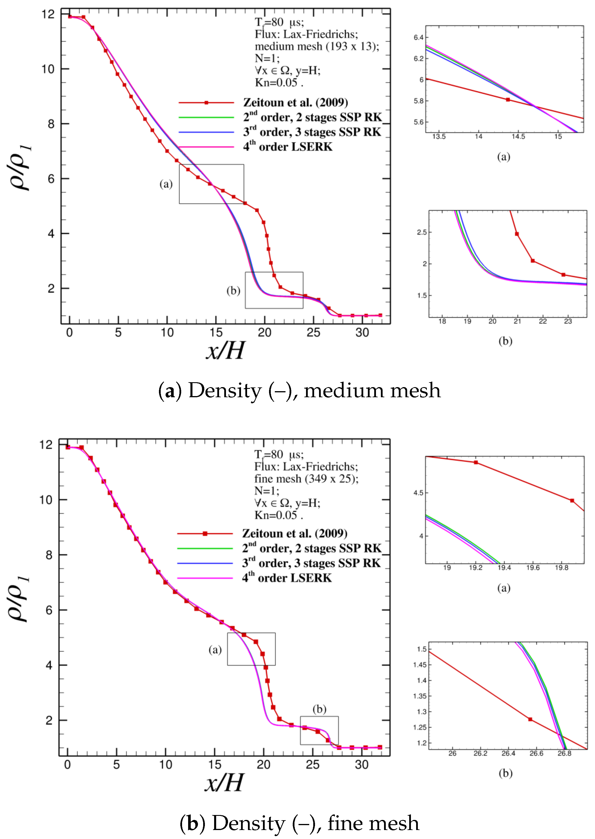
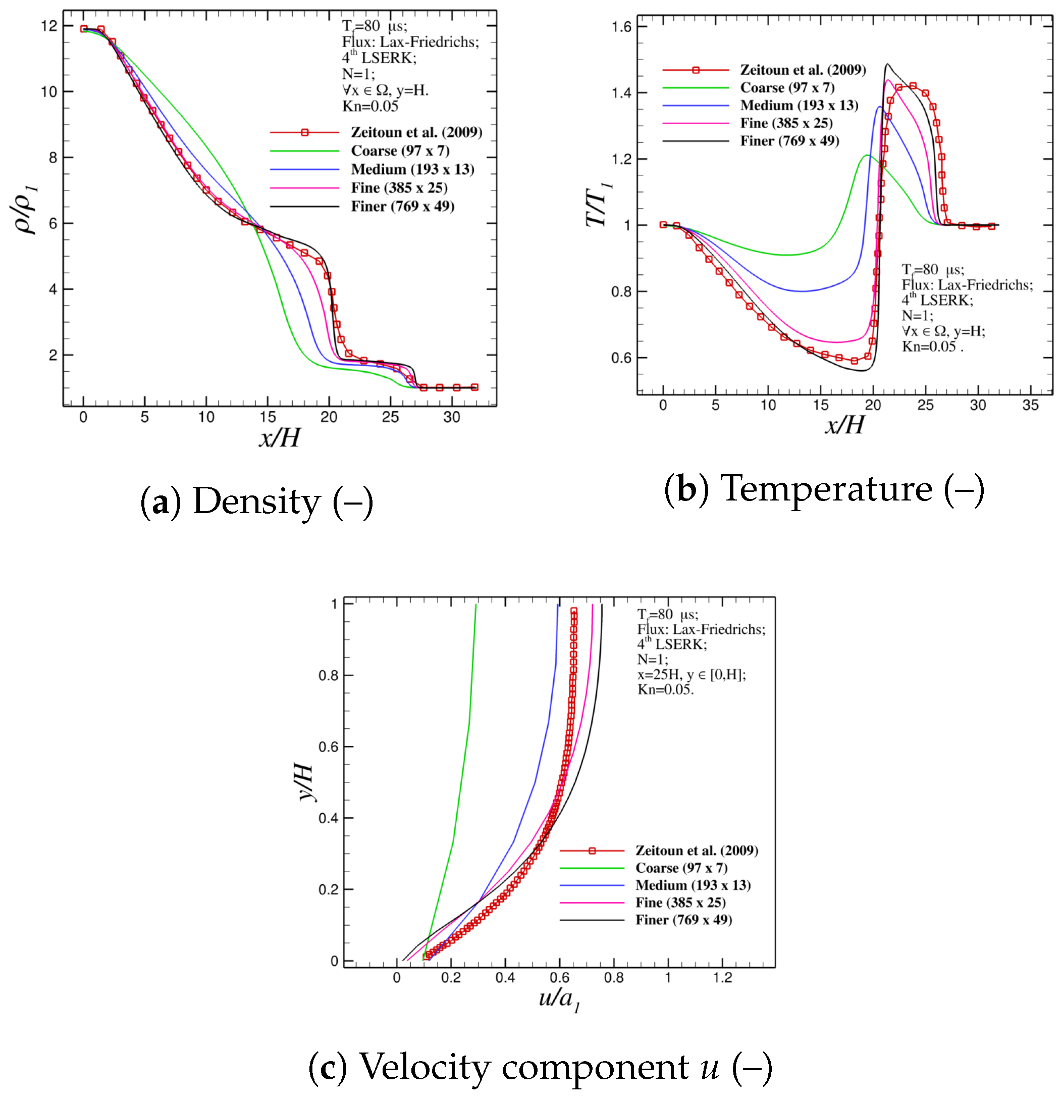
Figure 3a,b shows, respectively, the dimensionless density and temperature extracted at the centerline of the channel () plotted against the dimensionless coordinate. Qualitatively speaking, referring to the density profile in Figure 3a, one can see that the accuracy of the numerical results achieved increases when the mesh used is finer; in particular, with the coarse and medium mesh, the profile is very diffusive yielding to an incorrect and inaccurate representation of the discontinuities in the flow field. In fact, the density in the rarefaction wave region is over predicted and, as a result, the positions of the contact wave and of the shock wave are imprecise. The real flow physics is matched when the fine and finer mesh are considered, since less numerical diffusion can be observed and, as a result, the density jumps are properly caught. Analogous considerations can be done for the dimensionless temperature profile shown in Figure 3b. Firstly, one can observe that the accuracy quickly increases as the mesh is refined, in fact, for instance, the results achieved adopting the coarse mesh do not match at all the jumps in the flow field observed by Zeitoun et al. [21]. Furthermore, considering the finer grid level, it is observed that the position of the contact wave is properly achieved using DG–FEM, however the whole jump in temperature is slightly bigger than the one observed in the reference data (the relative error observed is approximately 10.6%). This produces a small under prediction of the shock wave position (relative error equal to 3.8%).
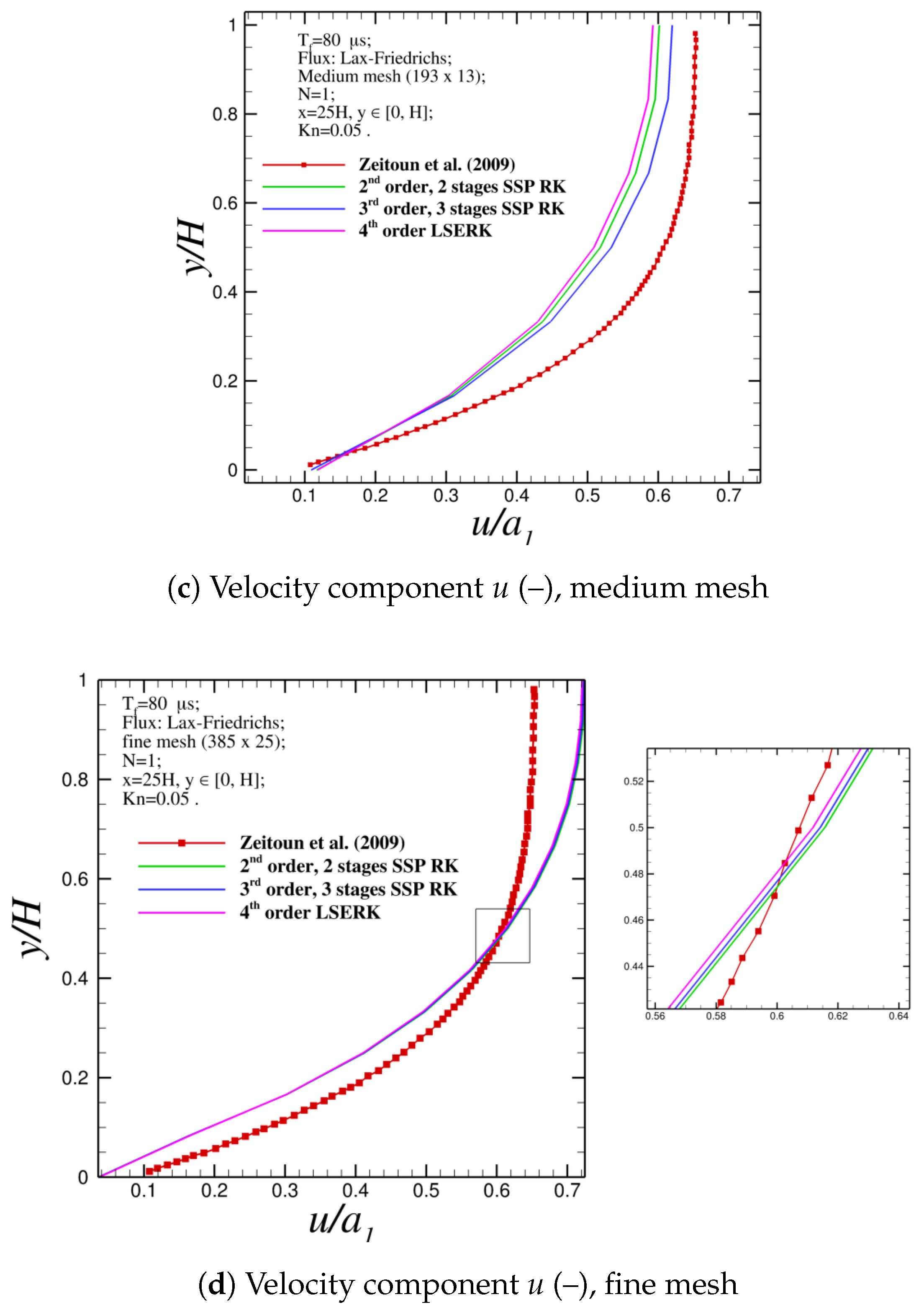
The numerical results are validate also in terms of streamwise velocity u (Figure 3c) in , which represents the position immediately before the shock wave (pre-shock state). The velocity is made dimensionless using the speed of sound in the driven chamber defined as and plotted against the dimensionless coordinate (for the first half of the channel’s height). The velocity profile obtained with the coarse and medium mesh under predicts the outcomes given by Zeitoun et al. [21], while bigger values are achieved adopting the fine and finer mesh; however, when , the profiles obtained overcome the reference data. The numerical results obtained for the stream wise velocity are quite accurate even if they are studied in the no slip fluid flow regime. However, as the Knudsen number increases, the slip condition becomes mandatory [19].
To confirm that the numerical results achieved grid convergence, a simulation on an additional grid level 5—which is the finest mesh—is performed to compare the results between the finer and the finest mesh (see Figure 4). The refinement ratio is kept equal to 2, so the finest grid level is characterized by and grid points in the x and y directions, respectively, and mesh widths mm. Figure 4 shows that the mesh further refinement does not improve significantly the already obtained accuracy of the numerical simulation results, which means that the further refinement of the mesh compared to the grid level 4 could increase the computational cost without significant further improvement of the achieved accuracy.
For the sake of a quantitative analysis, the , and norms of the absolute error between the numerical results and the reference data given by Zeitoun et al. [21] are computed. Figure 5 shows the logarithmic plots of the (Figure 5a), (Figure 5b) and (Figure 5c) norms of the absolute error between the results achieved with DG–FEM and reference data given by [21] against the inverse of the dimensionless grid spacing h. Regarding the density and the temperature, the three plots clearly show that as the mesh is refined, the error drops in terms of all the norms considered. The same trend can be observed for the velocity profile, however, going from the fine to the finer grid level, the error increases after . The reason is that the present investigation focuses on the low Knudsen number flow regime, where rarefaction effects start to become important but still not dominant. Rarefaction effects are taken into account in a continuum approach—i.e., using compressible Navier–Stokes equations—imposing wall slip boundary conditions producing hence a different velocity profile [19]. The slip boundary condition becomes a mandatory requirement as the Knudsen number increases, which would yield to more physical and accurate results as confirmed by other authors in [19,21] when other continuum based numerical approaches were employed as well. This behavior is also met in the qualitative discussion above, since it is seen that the velocity profile achieved through the finer mesh overcomes the reference data when . Furthermore, the lowest error norms are observed for the stream wise velocity profile extracted in . For the sake of a complete analysis, the error norms are also summarized in Table 4.
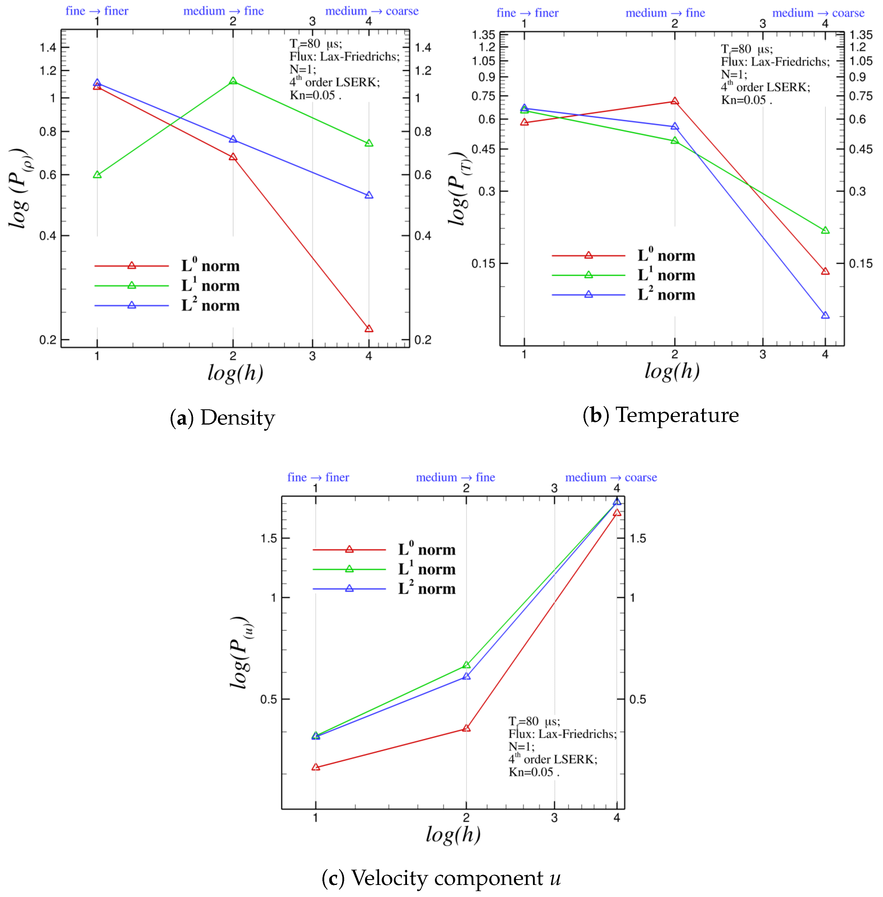
A convergence test is performed in order to understand if the formal order of accuracy matches (or not) the observed order of accuracy. Hence, within this approach, one can understand if the discretization error is reduced at the expected rate [30]. The formal order of accuracy can be achieved from a truncation error analysis, and, in the FEM approach, it is equal to N. In particular, in this case, since first-order polynomials are considered. The observed order of accuracy is computed from the numerical outputs on systematically refined grids [30]. The observed order of accuracy is based on the trend of the error. Consider two generic grid levels i and , being the i-th level the finer among them, and let and be the absolute errors for these grid levels. The observed order of accuracy, based on the norms of the errors is defined by
In this work, different grid levels are taken into account along with different observed orders of accuracy for each flow property and for each norms. Figure 6 shows three logarithmic plots of the observed order of accuracy adopting the , and norms of the absolute error between the results achieved with DG–FEM and reference data given by [21] against the dimensionless grid spacing h.
The simulations are performed using the first-order polynomial representation and, for a sake of clarity, the observed order of accuracy for each quantity, for each norm, is also listed in Table 5. Figure 6a shows that, regarding the density at the centerline of the microchannel, for the and norms, the observed order of accuracy increases as the mesh is refined, reaching the values 1.076 and 1.104, respectively, which are higher than the theoretical order . The same trend is not shared by the norm, which exhibits a maximum between the medium and fine grid level. Concerning the temperature profile (Figure 6b), all the values are below the theoretical order and the observed order increases as the mesh is refined for the and norms, while the norm shows a maximum between the medium and fine mesh. The stream wise dimensionless velocity profile in Figure 6c shows a different trend, which means that the observed order of accuracy decreases as the mesh is refined, as also confirmed by the previous discussions about Figure 3c and Figure 5.
3.2. Effect of Different Time Integration Schemes
The effect of different time integration schemes is investigated. The following explicit Runge–Kutta schemes are taken into account: second-order, two-stage SSP–RK, third-order, three-stage SSP–RK and fourth-order LSERK. The limiting procedure is applied for each stage of the methods. The investigation is performed adopting both the medium and fine mesh and Figure 7 shows the results obtained for density and streamwise velocity. Referring to Figure 7a,b, where the density profile is plotted, respectively, adopting the medium and fine mesh with the three RK schemes presented, no big differences are observed. On the right of the figures, some zooms are shown: a unique trend is not observed, with the medium mesh the accuracy of the second-order, two-stage SSP–RK is always between the other two schemes. When the fine mesh is used, the differences among the schemes become even smaller and the third-order, three-stage SSP–RK seems to hold an average trend among the other methods. Broadly speaking, the same trend can be observed for the stream wise velocity profiles in Figure 7c,d , where the medium and fine grids are used, respectively. When the medium mesh is used, the third-order, three-stage SSP–RK scheme gives the most accurate profile, while using the fine mesh the results achieved are very similar. In particular, the second-order, two-stage SSP–RK is more accurate in the first part of the profile and the fourth-order LSERK in the second.
Of course, one can see that, due to the small differences among the outputs obtained, a qualitative analysis cannot determine correctly which scheme yields to the most accurate results. Hence, as previously done, the , and norms of the absolute error are computed and listed in Table 6 for the medium and fine mesh. On the one hand, regarding the medium mesh, it is possible to observe that the third-order, three-stage SSP–RK scheme is the least accurate, since the lowest error norms are gotten. This behavior is met for all norms, for all the physical quantities considered. On the other hand, when the fine mesh is adopted, a unique trend is not observed: the fourth-order LSERK scheme is more accurate for temperature and density (except for the norm), while the second-order, two-stage SSP–RK is the most accurate for the stream wise velocity.
To understand exactly how those time integration schemes perform, the relative difference among the previous error norms is compared. In particular, the relative difference among different temporal schemes using the norms are defined by
where the superscripts , and , respectively, indicate the error norms computed using the second-order, two-stage SSP–RK, third-order, three-stage SSP–RK and fourth-order LSERK. These quantities are collected, in percentage, in Table 7. From the table, one can see that the relative difference is bigger when the medium mesh is adopted and this trend is emphasized when the stream wise velocity is taken into account. However, generally speaking, when the fine mesh is considered, the relative differences has as order of magnitude 1%, which can be considered a negligible outcome. For this reason, it is possible to conclude that when a fine (or even a finer) mesh is considered, the choice of the temporal scheme do not really affect the accuracy of the numerical results.
3.3. Effect of Different Time Step Sizes
The effect of different time step sizes on the accuracy of the numerical results is investigated. The time step size is computed using Equation (24) to get a stable solution according to [22]. The following time step sizes are considered: , , , and . The numerical simulations are performed using the fine mesh with second-order, two-stage SSP–RK scheme. Changing the time step size still gives stable and bounded solutions and relevant changes in terms of accuracy are not observed. The , and norms of the absolute error among reference data and numerical solutions are computed and it is observed that they share same precision up to the fourth digit. As for the temporal integration schemes study, the relative difference among the error norms is computed as:
The index j indicates a time step size level, in particular corresponds to and to . Table 8 shows these relative differences and it can be observed that the order of magnitude, in percentage, is between and . For this reason, it is possible to conclude that time step sizes do not affect the accuracy of the numerical solution.
4. Conclusions
The two-dimensional unsteady fully-compressible Navier–Stokes equations for microfluidic problems are numerically solved adopting the nodal discontinuous Galerkin finite element method (DG–FEM) in space and different explicit Runge–Kutta (RK) schemes for the temporal integrations. The equations are solved at microscale level considering a miniaturized version of the shock-channel problem as test case. Unstructured meshes are generated and a MATLAB code developed by Hesthaven and Warburton [22] is adopted, modified and further improved. The numerical results are validated with reference data provided by Zeitoun et al. [21] where CNS equations in a FVM context, DSMC for the Boltzmann equation and the kinetic model BGKS (Bhatnagar–Gross–Krook with Shakhov equilibrium distribution function) models are adopted. A mesh refinement study is performed using four grid levels. The study showed that, as the mesh is refined, more accurate results are achieved. This trend is always confirmed for the density and temperature profiles, while for the streamwise velocity profile, the error slightly increases from the fine to the finer mesh. In fact, when the finer grid is adopted, it is observed that the method overestimates the velocity profile. A slip boundary condition implementation could improve this result. The observed order of accuracy based on different error norms for different flow properties is also computed and it is shown that, when the first-order of polynomial is adopted (theoretical order of one), the following results are achieved: for the density and temperature, as the mesh is refined, the observed order of accuracy increases reaching (and overcoming for the density) the theoretical order; a different trend is achieved for the velocity profile, i.e., the order is higher as the mesh is coarser. The reason behind this behavior is the same as the previous one for the error norms. An additional grid level is then considered, and it is seen that the mesh further refinement does not improve significantly the already obtained accuracy. In addition to this, the effect of different temporal schemes (explicit Runge–Kutta) is investigated considering second-order, two-stage SSP–RK; third-order, three-stage SSP–RK; and fourth-order LSERK. A qualitative and quantitative analysis is done computing error norms and their relative differences, however no big differences among the schemes are observed as the mesh is refined and it is concluded that the choice of the temporal scheme does not really affect the accuracy of the numerical results, especially when fine meshes are used. Finally, different time step sizes have also been considered, and the solution remains stable and the accuracy unaffected.
Acknowledgments
The present research work was financially supported by the Centre for Computational Engineering Sciences at Cranfield University under project code EEB6001R. We would also like to acknowledge the constructive comments of the reviewers of the Aerospace journal.
Author Contributions
Alberto Zingaro and László Könözsy contributed equally to this paper.
Conflicts of Interest
The authors declare no conflict of interest.
Abbreviations
The following abbreviations are used in this manuscript:
| BC | Boundary Condition |
| BGKS | Bhatnagar–Gross–Krook with Shakhov equilibrium distribution function |
| CFD | Computational Fluid Dynamics |
| CNS | Compressible Navier–Stokes |
| DG–FEM | Discontinuous Galerkin Finite Element Method |
| DSMC | Direct Simulation Monte Carlo |
| ERK4 | Fourth-Order Four-Stage Explicit Runge–Kutta |
| FEM | Finite Element Method |
| FVM | Finite Volume Method |
| LSERK | Low Storage Explicit Runge–Kutta |
| MEMS | Microelectromechanical Systems |
| ODE | Ordinary Differential Equation |
| PDE | Partial Differential Equation |
| RK | Runge–Kutta |
| SSP–RK | Strong Stability–Preserving Runge–Kutta |
References
- Gribbin, J.; Gribbin, M. Richard Feynman: A Life in Science; Plume: New York, NY, USA, 1998. [Google Scholar]
- Gad-el-Hak, M. Use of Continuum and Molecular Approaches in Microfluidics. In Proceedings of the 3rd Theoretical Fluid Mechanics Meeting, St. Louis, MO, USA, 24–26 June 2002. [Google Scholar]
- Duff, R.E. Shock-Tube Performance at Low Initial Pressure. Phys. Fluids 1959, 2, 207–216. [Google Scholar] [CrossRef]
- Roshko, A. On Flow Duration in Low-Pressure Shock Tubes. Phys. Fluids 1960, 3, 835–842. [Google Scholar] [CrossRef]
- Mirels, H. Test Time in Low-Pressure Shock Tubes. Phys. Fluids 1963, 6, 1201–1214. [Google Scholar] [CrossRef]
- Mirels, H. Correlation Formulas for Laminar Shock Tube Boundary Layer. Phys. Fluids 1966, 9, 1265–1272. [Google Scholar] [CrossRef]
- Pant, J.C. Some Aspects of Unsteady Curved Shock Waves. Int. J. Eng. Sci. 1969, 7, 235–245. [Google Scholar] [CrossRef]
- Huilgol, R.R. Growth of Plane Shock Waves in Materials with Memory. Int. J. Eng. Sci. 1973, 11, 75–86. [Google Scholar] [CrossRef]
- Ting, T.C.T. Intrinsic Description of 3-Dimensional Shock Waves in Nonlinear Elastic Fluids. Int. J. Eng. Sci. 1981, 19, 629–638. [Google Scholar] [CrossRef]
- Shankar, R. On Growth and Propagation of Shock Waves in Radiation-Magneto Gas Dynamics. Int. J. Eng. Sci. 1989, 27, 1315–1323. [Google Scholar] [CrossRef]
- Suliciu, I. On Modelling Phase Transitions by Means of Rate-Type Constitutive Equations. Shock Wave Structure. Int. J. Eng. Sci. 1990, 28, 829–841. [Google Scholar] [CrossRef]
- Shi, Z.; Reese, J.M.; Chandler, H.W. The Application of a Shock Wave Model to Some Industrial Bubbly Fluid Flows. Int. J. Eng. Sci. 2000, 38, 1617–1638. [Google Scholar] [CrossRef]
- Bhardwaj, D. Formation of Shock Waves in Reactive Magnetogasdynamic Flow. Int. J. Eng. Sci. 2000, 38, 1197–1206. [Google Scholar] [CrossRef]
- Zel’dovich, Y.B.; Raizer, Y.P. Physics of Shock Waves and High-Temperature Hydrodynamic Phenomena; Hayes, W.D., Probstein, R.F., Eds.; Dover Publications, Inc.: Mineola, NY, USA, 2002. [Google Scholar]
- Smith, D.; Amitay, M.; Kibens, V.; Parekh, D.; Glezer, A. Modification of Lifting Body Aerodynamics Using Synthetic Jet Actuators. In Proceedings of the 36th AIAA Aerospace Sciences Meeting and Exhibit, Reno, NV, USA, 12–15 January 1998. Paper No.: 98-0209. [Google Scholar]
- Raman, G.; Raghu, S.; Bencic, T.J. Cavity Resonance Suppression Using Miniature Fluidic Oscillators. In Proceedings of the 5th AIAA/CEAS Aeroacoustics Conference, Seattle, WA, USA, 10–12 May 1999. Paper No.: 99-1900. [Google Scholar]
- Gad-el-Hak, M. The Fluid Mechanics of Microdevices—The Freeman Scholar Lecture. J. Fluids Eng. 1999, 121, 5–33. [Google Scholar] [CrossRef]
- Sushanta, K.M.; Suman, C. Microfluidics and Nanofluidics Handbook: Fabrication, Implementation and Applications; CRC Press: Boca Raton, FL, USA, 2011. [Google Scholar]
- Karniadakis, G.; Beskok, A.; Aluru, N. Microflows and Nanoflows: Fundamentals and Simulation; Springer: New York, NY, USA, 2005. [Google Scholar]
- Brouillette, M. Shock Waves at microscales. Shock Waves 2003, 13, 3–12. [Google Scholar] [CrossRef]
- Zeitoun, D.E.; Burtschell, Y.; Graur, I.A.; Ivanov, M.S.; Kudryavtsev, A.N.; Bondar, Y.A. Numerical Simulation of Shock Wave Propagation in Microchannels Using Continuum and Kinetic Approaches. Shock Waves 2009, 19, 307–316. [Google Scholar] [CrossRef]
- Hesthaven, J.S.; Warburton, T. Nodal Discontinuous Galerkin Methods: Alghoritms, Analysis, and Applications; Springer: New York, NY, USA, 2008. [Google Scholar]
- Peraire, J.; Nguyen, N.C.; Cockburn, B. A Hybridizable Discontinuous Galerkin Method for the Compressible Euler and Navier-Stokes Equations. In Proceedings of the 48th AIAA Aerospace Sciences Meeting Including the New Horizons Forum and Aerospace Exposition, Orlando, FL, USA, 4–7 January 2010; pp. 1–11. [Google Scholar]
- Gottlieb, S.; Shu, W.; Tadmor, E. Strong Stability Preserving High Order Time Discretization Methods. SIAM Rev. 2001, 43, 89–112. [Google Scholar] [CrossRef]
- Carpenter, M.H.; Kennedy, C. Fourth-Order 2N–Storage Runge–Kutta Schemes. NASA Report TM 109112; NASA Langley Research Center: Hampton, VA, USA, 1994. [Google Scholar]
- Tu, S.; Aliabadi, S. A Slope Limiting Procedure in Discontinuous Galerkin Finite Element Method for Gasdynamics Application. Int. J. Numer. Anal. Model. 2005, 2, 163–178. [Google Scholar]
- Kennard, E.H. Kinetic Theory of Gases; McGraw–Hill: New York, NY, USA, 1938. [Google Scholar]
- Kandlikar, S.G.; Garimella, S.; Li, D.; Colin, S.; King, M.R. Heat Transfer and Fluid Flow in Minichannels and Microchannels; Elsevier: Oxford, UK, 2006. [Google Scholar]
- Bird, G.A. Monte Carlo simulation of gas flows. Annu. Rev. Fluid. Mech. 1978, 10, 11–31. [Google Scholar] [CrossRef]
- Veluri, S.P. Code Verification and Numerical Accuracy Assessment for Finite Volume CFD Codes. Ph.D. Thesis, Virginia Polytechnic Institute, Blacksburg, VA, USA, 2010. [Google Scholar]
Figure 1.
Different flow regimes in function of the Knudsen number .

Figure 2.
The sketch of the viscous shock-channel of Zeitoun et al. [21] for microfluidic applications.
Figure 2.
The sketch of the viscous shock-channel of Zeitoun et al. [21] for microfluidic applications.
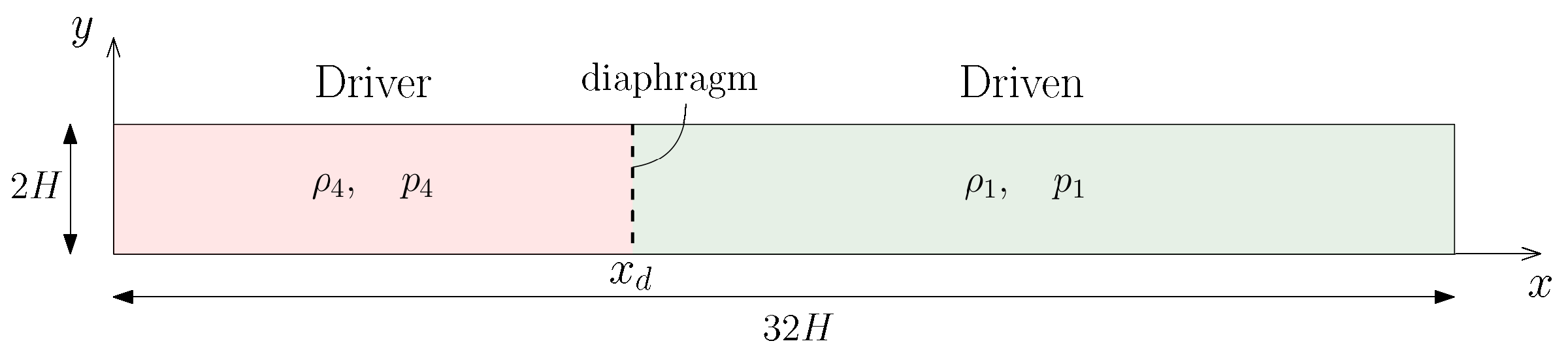
Figure 3.
Dimensionless density (a); temperature (b) profiles in the centerline of the microchannel; and stream wise velocity u (c) in the cross section using four grid levels at the final time s with in comparison with reference data of Zeitoun et al. [21].
Figure 3.
Dimensionless density (a); temperature (b) profiles in the centerline of the microchannel; and stream wise velocity u (c) in the cross section using four grid levels at the final time s with in comparison with reference data of Zeitoun et al. [21].

Figure 4.
Dimensionless density (a); temperature profiles (b) in the centerline of the microchannel; and stream wise velocity u (c) in the cross section on the finer and the finest grid levels at the final time s with .
Figure 4.
Dimensionless density (a); temperature profiles (b) in the centerline of the microchannel; and stream wise velocity u (c) in the cross section on the finer and the finest grid levels at the final time s with .
Figure 5.
, and norms of the absolute error between the results achieved with DG–FEM and reference data in [21] against the inverse of the dimensionless grid spacing h. Results presented for density and temperature in the centerline of the microchannel and stream wise velocity in the cross section . Results obtained at the final time s with .
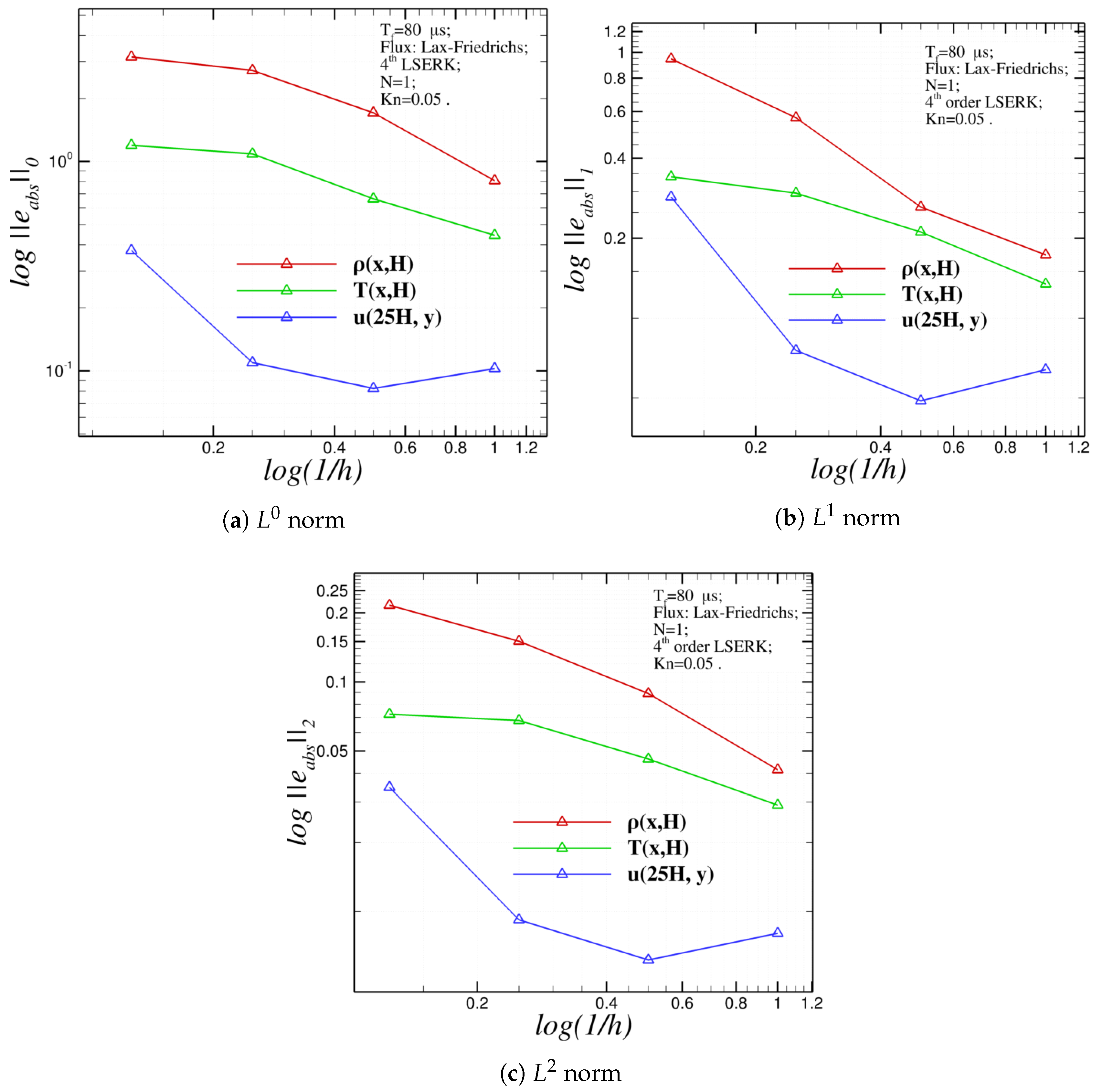
Figure 6.
Logarithmic plots of the observed order of accuracy using the , and norms of the absolute error between the results achieved with DG–FEM and reference data in [21] against the dimensionless grid spacing h. Results presented for: density (a); temperature (b) in the centerline of the microchannel; and streamwise velocity (c) in the cross section . Results obtained at the final time s with .

Figure 7.
Dimensionless density profile in the centerline of the microchannel (a,b); and streamwise velocity u in the cross section (c,d) using the: medium (a,c); and fine (b,d) mesh at the final time s with and . Comparison between different explicit Runge–Kutta schemes: second-order, two-stage SSP–RK, third-order, three-stage SSP–RK, and fourth-order LSERK. Validation with reference data of Zeitoun et al. [21].

Table 1.
Coefficients , and used for the low storage five-stage fourth-order explicit Runge–Kutta method.
Table 1.
Coefficients , and used for the low storage five-stage fourth-order explicit Runge–Kutta method.
| i | |||
|---|---|---|---|
| 1 | 0 | 0 | |
| 2 | |||
| 3 | − | ||
| 4 | |||
| 5 |
Table 2.
Zeitoun’s test case: geometric information and output time for the simulation (a); flow properties in the driver and driven chambers (b); and Argon properties in standard condition (c).
Table 2.
Zeitoun’s test case: geometric information and output time for the simulation (a); flow properties in the driver and driven chambers (b); and Argon properties in standard condition (c).
| (a) | ||
| characteristic length H (mm) | 2.5 | |
| size of the domain (mm) | ||
| diaphragm position (mm) | 29.60 | |
| Output time (s) | 80 | |
| (b) | ||
| Left | Right | |
| Driver | Driven | |
| state | 4 | 1 |
| Gas | Ar | Ar |
| (kg/m) | 8.43 × 10 | 7.08 × 10 |
| u (m/s) | 0 | 0 |
| v (m/s) | 0 | 0 |
| p (Pa) | 525.98 | 44.2 |
| (c) | ||
| specific gas constant R (J/(kg·K)) | 208.0 | |
| specific heat ratio (–) | 1.67 | |
| thermal conductivity (W/(m·K)) | 0.0172 | |
| Sutherland’s reference viscosity (kg/(m·s)) | 2.125 × | |
| Sutherland’s reference temperature (K) | 273.15 | |
| Sutherland’s temperature C (K) | 144.4 | |
Table 3.
Grid levels adopted in the mesh refinement study.
| Mesh | Level i | (mm) | (mm) | h (–) | (–) | ||
|---|---|---|---|---|---|---|---|
| Coarse | 4 | 97 | 7 | 8.33 × | 8.33 × | 8 | 0.125 |
| Medium | 3 | 193 | 13 | 4.17 × | 4.17 × | 4 | 0.25 |
| Fine | 2 | 385 | 25 | 2.08 × | 2.08 × | 2 | 0.5 |
| Finer | 1 | 769 | 49 | 1.04 × | 1.04 × | 1 | 1 |
Table 4.
, and norms of the absolute error between the results achieved with DG–FEM and reference data in [21]. Results presented for density (a), temperature (b) in the centerline of the microchannel, and stream wise velocity (c) in the cross section . Results obtained at the final time s with .
Table 4.
, and norms of the absolute error between the results achieved with DG–FEM and reference data in [21]. Results presented for density (a), temperature (b) in the centerline of the microchannel, and stream wise velocity (c) in the cross section . Results obtained at the final time s with .
| (a) Density | ||||
| Coarse | Medium | Fine | Finer | |
| (–) | 3.15963 | 2.72327 | 1.70752 | 0.81022 |
| (–) | 0.94709 | 0.56817 | 0.26207 | 0.17318 |
| (–) | 0.21601 | 0.15045 | 0.08903 | 0.04143 |
| (b) Temperature | ||||
| Coarse | Medium | Fine | Finer | |
| (–) | 1.19697 | 1.08770 | 0.66427 | 0.44463 |
| (–) | 0.34085 | 0.29573 | 0.21112 | 0.13444 |
| (–) | 0.07237 | 0.06797 | 0.04617 | 0.02911 |
| (c) Velocity Component | ||||
| Coarse | Medium | Fine | Finer | |
| 0.37619 | 0.10962 | 0.08258 | 0.10261 | |
| 0.28596 | 0.07559 | 0.04886 | 0.06401 | |
| 0.03477 | 0.00921 | 0.00615 | 0.00804 | |
Table 5.
Observed order of accuracy for density, temperature and u velocity based on , and norms of the absolute error between numerical solution obtained with DG–FEM and numerical data in [21].
Table 5.
Observed order of accuracy for density, temperature and u velocity based on , and norms of the absolute error between numerical solution obtained with DG–FEM and numerical data in [21].
| Grid Level (from → to) | 1 → 2 | 2 → 3 | 3 → 4 | 1 → 2 | 2 → 3 | 3 → 4 | 1 → 2 | 2 → 3 | 3 → 4 |
|---|---|---|---|---|---|---|---|---|---|
| (–) | 1.076 | 0.673 | 0.214 | 0.579 | 0.711 | 0.138 | 0.313 | 0.409 | 1.779 |
| (–) | 0.598 | 1.116 | 0.737 | 0.651 | 0.486 | 0.205 | 0.390 | 0.629 | 1.920 |
| (–) | 1.104 | 0.757 | 0.522 | 0.666 | 0.558 | 0.091 | 0.387 | 0.582 | 1.917 |
Table 6.
, and norms of the absolute error between the results achieved with DG–FEM and reference data in [21]. Comparison between different explicit RK schemes using the medium and fine mesh. Results presented for density (a); temperature (b) in the centerline of the microchannel; and stream wise velocity (c) in the cross section . Results obtained at the final time s with and .
| (a) Density (–) | ||||||
| Medium | Fine | |||||
| –order, 2 stage SSP–RK | 2.7233 | 0.5682 | 0.1505 | 1.7075 | 0.2621 | 0.0890 |
| –order, 3 stage SSP–RK | 2.6024 | 0.5333 | 0.1442 | 1.6846 | 0.2566 | 0.0874 |
| –order LSERK | 2.6870 | 0.5563 | 0.1484 | 1.6689 | 0.2530 | 0.0862 |
| (b) Temperature (–) | ||||||
| Medium | Fine | |||||
| –order, 2 stage SSP–RK | 1.0877 | 0.2957 | 0.0680 | 0.6643 | 0.2111 | 0.0462 |
| –order, 3 stage SSP–RK | 1.0480 | 0.2817 | 0.0658 | 0.6465 | 0.2086 | 0.0454 |
| –order LSERK | 1.0756 | 0.2912 | 0.0673 | 0.6348 | 0.2070 | 0.0448 |
| (c) Velocity Component (–) | ||||||
| Medium | Fine | |||||
| –order, 2 stage SSP–RK | 0.1096 | 0.0756 | 0.0092 | 0.0826 | 0.0489 | 0.00615 |
| –order, 3 stage SSP–RK | 0.0903 | 0.0585 | 0.0072 | 0.0833 | 0.0494 | 0.00622 |
| –order LSERK | 0.1019 | 0.0692 | 0.0084 | 0.0834 | 0.0496 | 0.00625 |
Table 7.
Relative difference among , and norms of the absolute error achieved using second-order, two-stage SSP–RK, third-order, three-stage SSP–RK and fourth-order LSERK scheme. Results obtained using the medium and fine mesh density and temperature in the microchannel’s centerline and stream wise velocity in the cross section . Results obtained at the final time s with and .
| Medium Mesh | Fine Mesh | ||||||
|---|---|---|---|---|---|---|---|
| (%) | 4.43947 | 6.14220 | 4.18605 | 1.34233 | 2.07547 | 1.88136 | |
| (%) | 3.25085 | 4.31277 | 2.91262 | 0.93030 | 1.39436 | 1.27821 | |
| (%) | 3.64473 | 4.73038 | 3.15965 | 2.67499 | 1.17253 | 1.76798 | |
| (%) | 2.63372 | 3.35658 | 2.23801 | 1.81116 | 0.79209 | 1.17433 | |
| (%) | 17.66372 | 22.60352 | 21.77167 | 0.90700 | 1.09284 | 1.11081 | |
| (%) | 12.92501 | 18.20015 | 17.17119 | 0.93030 | 1.39436 | 1.27821 | |
Table 8.
Relative difference among , and norms of the absolute error achieved using different time step sizes. Results obtained with fine mesh and second-order, two-stage SSP–RK scheme and shown for density and temperature in the centerline of the microchannel and stream wise velocity in the cross section . Results obtained at the final time s with and .
| (%) | (%) | (%) | (%) | ||
|---|---|---|---|---|---|
| 2.8756 × | 1.6312 × | 1.4415 × | 1.2184 × | ||
| 2.8834 × | 1.6530 × | 4.3485 × | 6.1623 × | ||
| 1.4868 × | 8.4653 × | 6.8205 × | 9.2102 × | ||
| 3.0293 × | 3.8387 × | 1.9821 × | 1.0443 × | ||
| 3.0859 × | 3.9217× | 6.3271 × | 6.3682 × | ||
| 1.3106 × | 1.6615 × | 7.3049 × | 1.0169 × | ||
| 1.2996 | 1.6198 × | 1.2461 × | 1.0256 × | ||
| 5.6303 × | 7.0370 × | 5.4373 × | 4.4575 × | ||
| 7.6356 × | 9.5516 × | 7.3887 × | 6.0460 × |
© 2018 by the authors. Licensee MDPI, Basel, Switzerland. This article is an open access article distributed under the terms and conditions of the Creative Commons Attribution (CC BY) license (http://creativecommons.org/licenses/by/4.0/).
Share and Cite
MDPI and ACS Style
Zingaro, A.; Könözsy, L. Discontinuous Galerkin Finite Element Investigation on the Fully-Compressible Navier–Stokes Equations for Microscale Shock-Channels. Aerospace 2018, 5, 16. https://doi.org/10.3390/aerospace5010016
AMA Style
Zingaro A, Könözsy L. Discontinuous Galerkin Finite Element Investigation on the Fully-Compressible Navier–Stokes Equations for Microscale Shock-Channels. Aerospace. 2018; 5(1):16. https://doi.org/10.3390/aerospace5010016
Chicago/Turabian StyleZingaro, Alberto, and László Könözsy. 2018. "Discontinuous Galerkin Finite Element Investigation on the Fully-Compressible Navier–Stokes Equations for Microscale Shock-Channels" Aerospace 5, no. 1: 16. https://doi.org/10.3390/aerospace5010016
Note that from the first issue of 2016, this journal uses article numbers instead of page numbers. See further details here.