Robust Control Design for Quad Tilt-Wing UAV


Department of Aerospace Engineering, Nihon University, Chiba 274-8501, Japan
*
Author to whom correspondence should be addressed.
Aerospace 2018, 5(1), 17; https://doi.org/10.3390/aerospace5010017
Submission received: 8 December 2017
/
Revised: 30 January 2018
/
Accepted: 2 February 2018
/
Published: 7 February 2018
(This article belongs to the Special Issue Aircraft Dynamics & Control)
Abstract
:This paper describes the design method of a flight control system of a Quad Tilt-Wing (QTW) Unmanned Aerial Vehicle (UAV). A QTW-UAV is necessary to design a controller considering its nonlinear dynamics because of the appearance of the nonlinearity during transition flight between hovering and level flight. A design method of a flight control system using Dynamic Inversion (DI) that is one of linearization method has been proposed for the UAV. However, the design method based on an accurate model has a possibility of deterioration of control performance and system stability. Therefore, we propose a flight control system that considers uncertainties such as modeling error and disturbances by applying an H-infinity controller to the linearized system. The validity of the proposed control system is verified through numerical simulation and experiment.
1. Introduction
Unmanned Aerial Vehicles (UAVs) are expected to be used as a tool for various missions including search, observation, inspection, mapping, and rescue in the event of a disaster [1,2]. UAV is generally classified into fixed-wing UAVs [3] and rotary-wing UAVs. A fixed-wing UAV is appropriate for a mission to search or inspect broad area because of low fuel consumption and high cruising speed. However, a fixed-wing UAV cannot move sensitively and intricately [4,5] including hovering, backward and sideward flight, and take-off without runway. A Quad Tilt-Wing (QTW) UAV that has advantages of a fixed wing and a rotary wing UAV and has been the focus of research in the last decade [6,7,8,9,10,11,12,13,14].
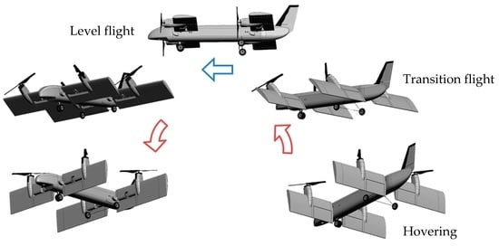
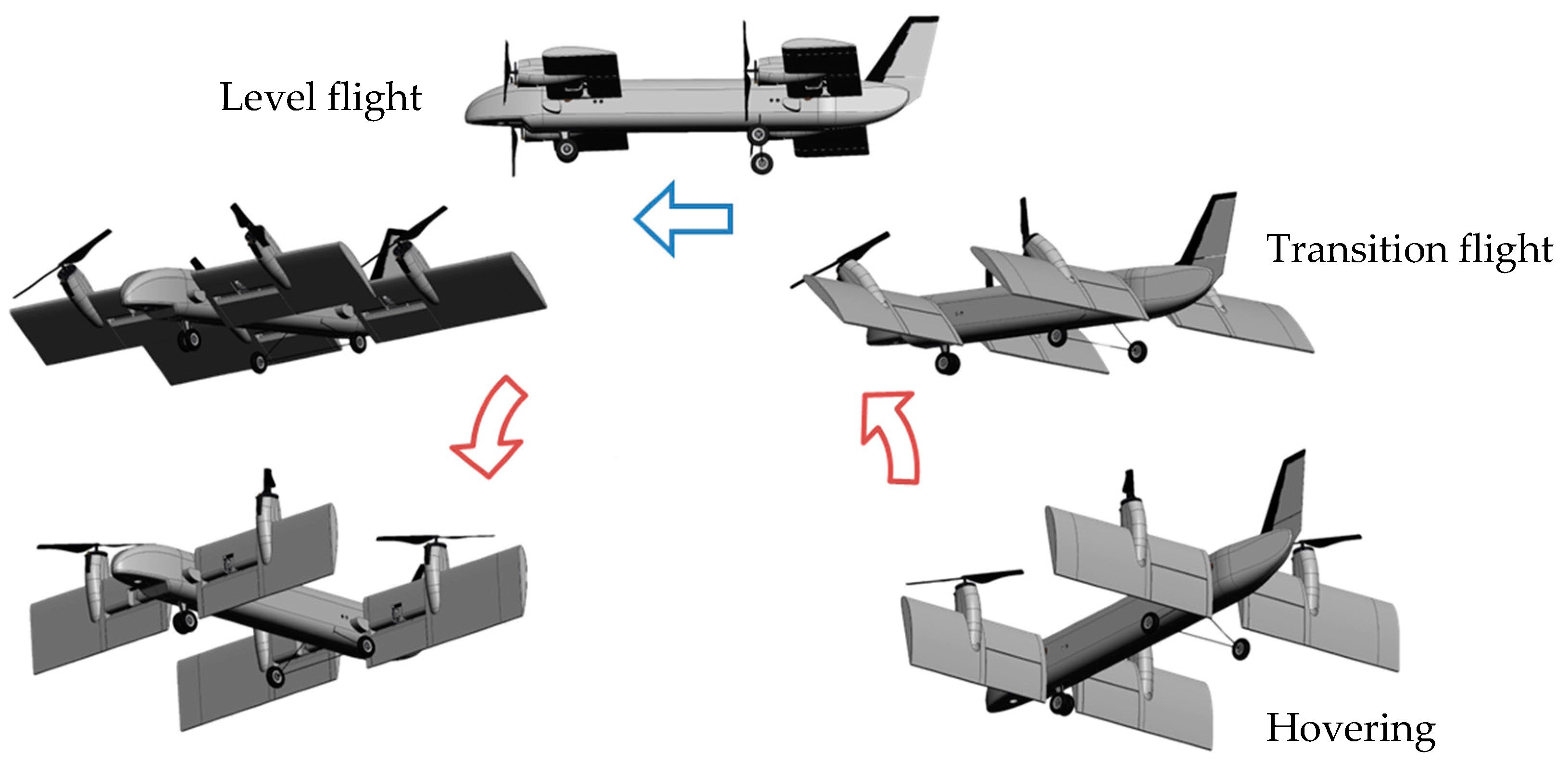
A QTW-UAV has four rotors fixed at wings that can be tilted. Its flight configuration is shown in Figure 1. Specifically, the UAV can hover and perform vertical takeoff and landing in multicopter mode at the tilt angle of 90 degrees and cruises in fixed-wing mode at the tilt angle of 0 degrees. Dynamics of a QTW-UAV changes significantly with strong nonlinearity by a change of the tilt angle. In particular, it is difficult to control its attitude and to guarantee system stability during transition flight. A Gain Scheduling (GS) controller that would be one of the useful methods for the UAV was designed [9,10]. It is quite difficult to adjust controller gains for linearized model around equilibrium states depending on the variation of the tilt angle and velocity of the UAV. Furthermore, the discontinuous change of controller gains would result in deterioration of control performance and system instability during its flight. Although the method of improving robustness by combining GS controller and robust output regulator has also been proposed, system instability by discontinuous change cannot be solved [12]. On the other hand, a design method with non-switching controller gain was proposed to overcome the problem [13]. An optimal controller was designed for a Linear Parameter-Varying model whose system matrix varies with the tilt angle. Although the controller gain changes continuously, it is difficult to control the UAV in real time because the Riccati equation should be solved to obtain the gain. Mikami [14] proposed a flight control system without the use of any approximation algorithms for its dynamics. It is easy to design a controller because the linear model can be obtained by using the Dynamic Inversion (DI) method. The validity of the design method was certainly verified numerically. However, the DI method needs an accurate model to guarantee the system stability. This means that the proposed flight control system does not have robustness against uncertainties because aerodynamic coefficients, which vary with the tilt angle, should be identified beforehand. Moreover, it would be also difficult to control the UAV in real time because of calculation complexity to obtain the linearized model. Conventional flight control systems for the UAV were basically designed assuming an accurate dynamical model. In addition, it cannot be considered that there is no effect of wind disturbance on dynamical behavior of small UAVs that have been developed actively. There is the necessity of a flight control system possessing robustness against uncertainties for the UAV.
We propose the design method of a robust control system considering uncertainties for a QTW-UAV. Its dynamics is expressed by nonlinear equations of translational motion and rotational motion. Then, controllers of each motion are designed separately. The equations motion is linearized by the DI method when designing a flight control system. The main objective of this study is to compensate robust stability during a flight of the UAV. Therefore H-infinity is applied to only the rotational motion so as to have robustness against disturbance such as wind. An optimal control method is applied to the rotational motion in this paper. An observer based on the Disturbance Accommodation Control (DAC) method is employed to estimate a disturbance and nonlinear term in its dynamics [15,16]. Moreover, the QTW-UAV is developed to verify the validity of the proposed flight control system.
2. Dynamics of the QTW-UAV
2.1. Variables and Coordinate Definition
Figure 2 shows state variables and control inputs of the QTW-UAV. The inertial coordinate system is fixed at the surface of the earth. The origin of the body coordinate system coincides with the center of mass of the QTW-UAV. , , and represent velocities of the QTW-UAV along , , and axis, respectively , , and are angular velocities around each axis. The position and attitude of the QTW-UAV are controlled by thrust , , , and generated by propellers. Flaperons, which are attached at wings behind each propeller, generate force to the vertical direction to wing by vectoring thrust. Flaperons’ angles are denoted by , , , and . Parameters and are tilt angles for the front wing and rear wing, respectively. Tilt angles can vary from 0 degrees to 90 degrees.
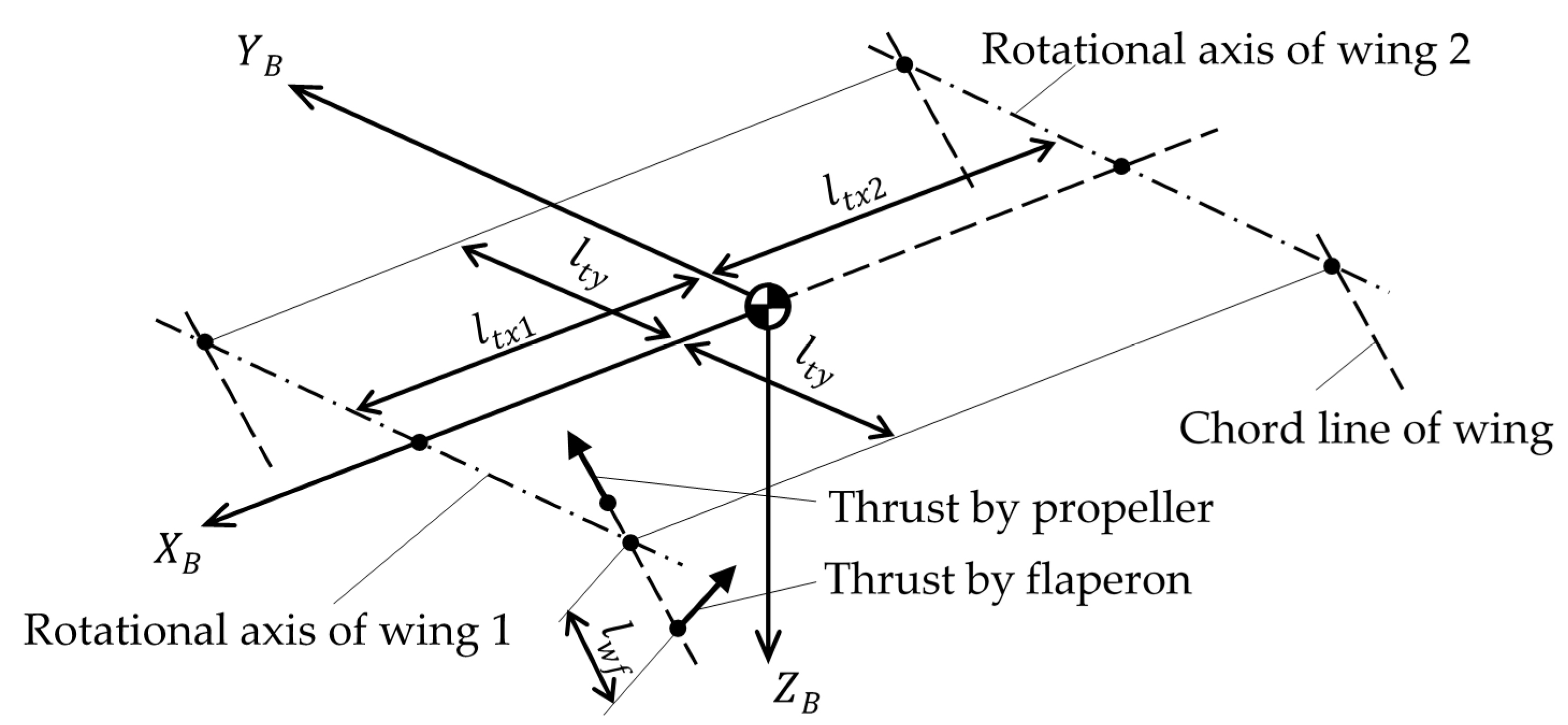
The arrangement of the propellers and flaperons is shown in Figure 3. is the distance from the rotational axis of the wing to the point of the application of thrust generated by flaperon. , , and denote the distance from the center of mass of QTW-UAV to the point of the application of thrust generated by propeller along each axis.
2.2. Nonlinear Equations of Motion
The nonlinear equations of translational and rotational motion are expressed, respectively, as follows:
The vectors and matrices in the above equations are defined as
where air force is a function of angle of attack and tilt angle . and are lift and drag forces of the front wing (wing 1). and are lift and drag forces of rear wing (wing 2). These forces are expressed by the following equations.
Similarly, and are lift and drag forces of body as follows:
The force generated by flaperon is expressed as
where is dynamic pressure occurred to each flaperon given by velocity of UAV. is the dynamic pressure that is generated by a propeller as follows:
is the propeller slipstream given by the relationship between thrust and square of the rotational plane.
The propeller generates thrust and anti-torque. Thus, it is required to consider moment by anti-torque when the propeller is rotated. Generally, propeller thrust and anti-torque are defined as proportional to square of angular velocity of an actuator.
Finally, in order to calculate anti-torque to thrust, the angular velocity of propeller is obtained from the following equation.
3. Design of Flight Controller
The proposed flight control system consists of a translational controller and a rotational controller. Figure 4 shows a block diagram of the proposed flight control system.
3.1. Translational Controller
The position error is defined as
where is the current position, and the desired position that is command value to the translational controller.
The second derivative of the QTW-UAV is obtained by using the transform matrix , velocity vector V. Here, the subscript of the coordinate transformation matrix represents the conversion from the body coordinate system to the inertial coordinate system.
Substituting the translational motion Equation (1) into above equation, the following equation is obtained.
The nonlinear term is estimated by the observer based on the DAC method [15,16]. The term is assumed here to be a polynomial of time with coefficients and that are not necessary to calculate directly. Then, its time derivative and second order derivative can be defined as follows:
The estimated value of the position error can be obtained as follows:
in which the observer gain is . The observation value that is position and velocity obtained by sensors such as an accelerometer is denoted by. is the estimated output vector. The symbol means an estimated value. The observable states are position and velocity. The following equation is derived from Equations (22) and (23).
The Linear Quadratic (LQ) method is applied to a duality system of Equation (24) to design the observer gain. The input vector for linearizing the error equation by using the DI method is expressed by the equation including estimated nonlinear terms as follows:
where is a new control input of the linearized system. Assuming that the estimated nonlinear term agrees with its true value completely, the equation of the error relating to translational motion is obtained.
Equation (27) is rewritten by the state equation.
Assume a state feedback of the form for the control input .
The feedback gain is designed by using LQ method.
Figure 5 shows a block diagram of the proposed control system for the translational motion of the UAV.
3.2. Rotational Controller
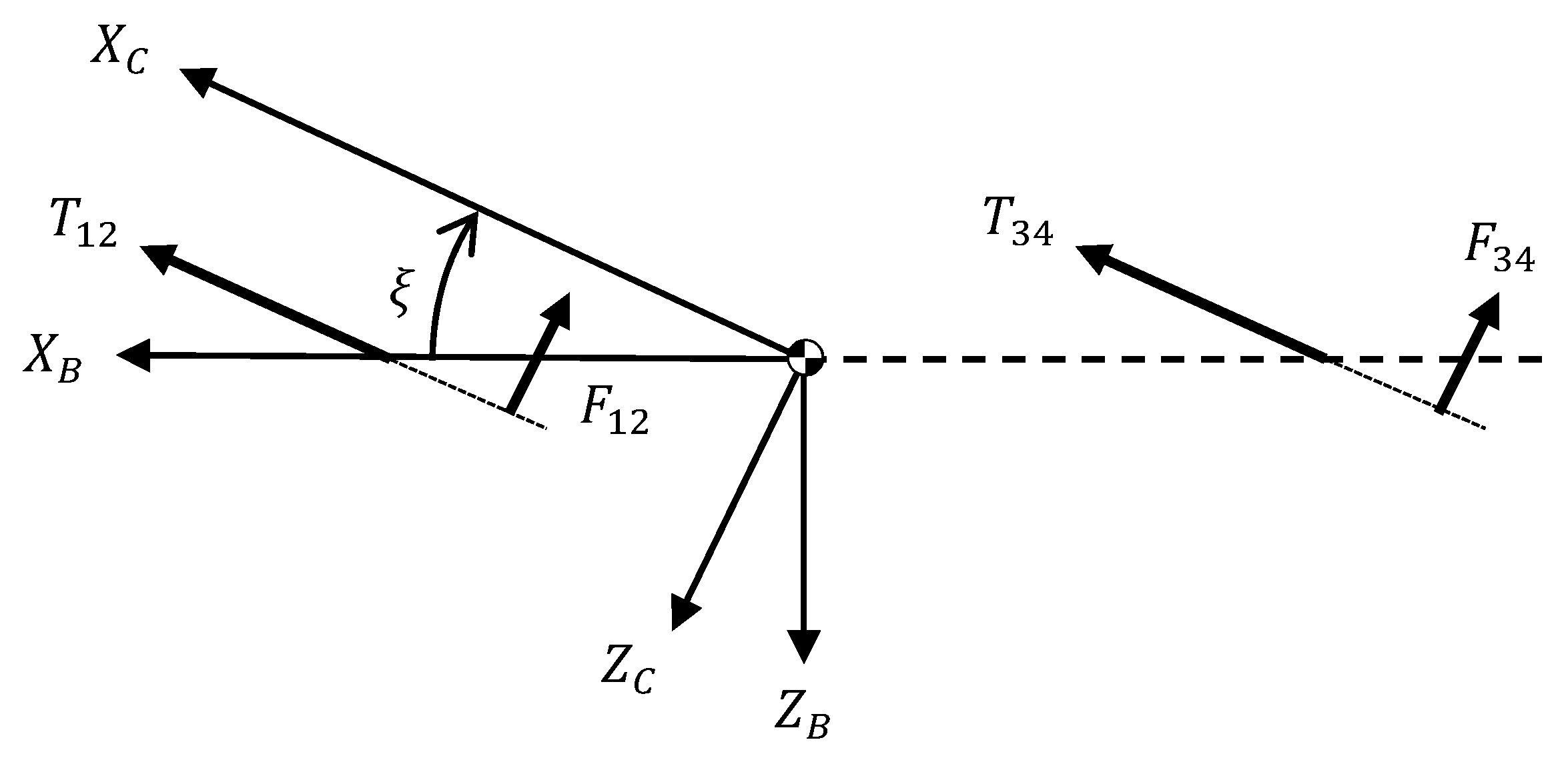
Euler angle commands for the rotational controller can be calculated from the components of as shown in Figure 6.
The tilt angle command and roll angle command are defined by the components, respectively, as
For simplicity, it assumed that the tilt angle of the front wing and the tilt angle of the rear wing commands are same value, and commands of pitch angle and azimuth angle are 0 degrees when calculating above commands in Equation (30).
The attitude error is obtained from the difference in a current attitude and desired attitude.
Differentiating Equation (31), the attitude of the UAV expressed by using Euler angle kinematics can be obtained.
Here, is the transform matrix as shown below.
Therefore, substituting the equation of rotational motion given by Equation (2) into Equation (32), the following equation is obtained.
The nonlinear term should be estimated by using the DAC observer because moment vector including aerodynamic force is generally an unknown parameter. is assumed to be a polynomial of time .
Equation (34) can be rewritten by using the estimated value of the DAC observer.
in which the observer gain is . and are the observation values, which are the angle and its derivative obtained by a gyro sensor, and the estimated output vector, respectively. The observable states are attitude and angular velocity. The following equation is derived from Equations (35) and (36).
The observer gain is designed by LQ method. The moment vector for linearizing the error equation by applying the DI method is expressed by the following equation including nonlinear terms estimated by the observer as follows:
where is regarded as a new control input of the linearized system. If nonlinear term that includes aerodynamic force in Equation (34) is accurately calculated, the nonlinear term in the rotational motion is completely canceled as Equation (40). In addition, the equation of rotational motion is rewritten as Equation (41).
It is noted that the uncertainty as estimated error in Equation (42) should be considered since the error actually occurs.
Therefore, the nonlinear term cannot completely be canceled even if DI method is applied to this system. Considering the above, Equations (40) and (41) are rewritten as follows:
The estimated error would lead to deterioration of control performance and instability of the system because LQ controller lacks robust property to cope with parameter perturbation or external disturbances.
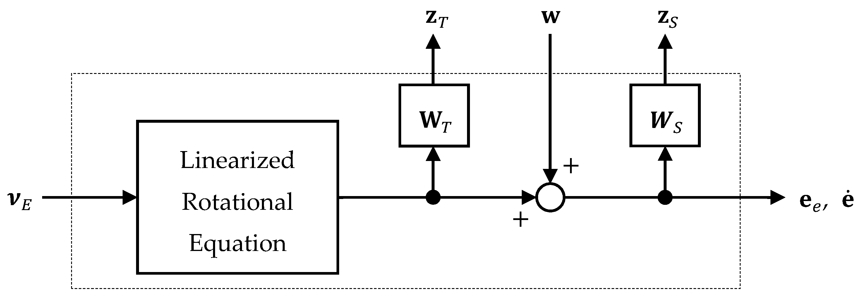
To overcome the problem, H-infinity controller is applied to the rotational motion of the UAV. Generalized plant of the system is as shown in Figure 7. Inversion error caused by estimated error is treated as a multiplicative uncertainty. The proposed H-infinity controller based on the mixed sensitivity reduction problem is designed to suppress not only the influence of the uncertainty such as inversion error but also disturbances of wind and sensor noise.
In Figure 7, is disturbance input, is evaluation output, is a weighting function of multiplicative uncertainty in a frequency domain, and is a frequency weighting function for reducing the influence of output the disturbance. Linear Matrix Inequality (LMI) solver is used to obtain the controller gain . The control input is defined as
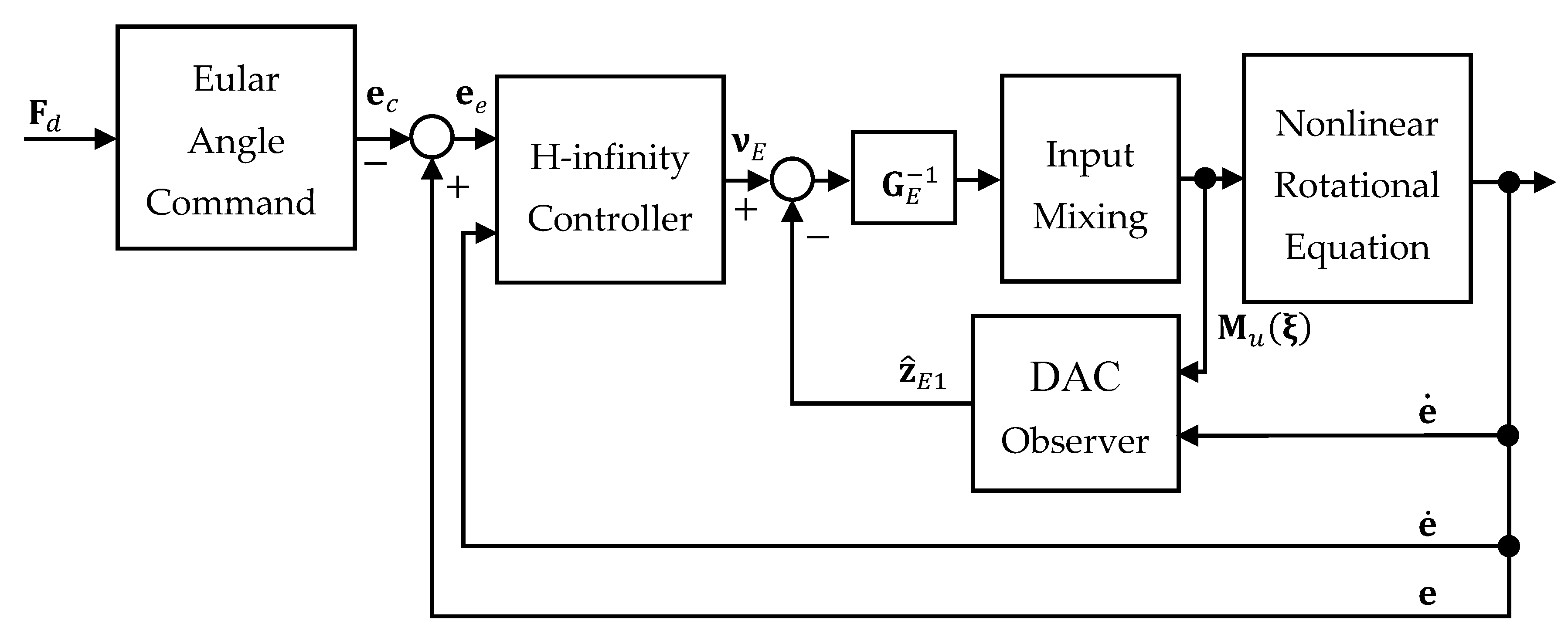
Figure 8 shows a block diagram of the proposed rotational control system.
3.3. Input Mixing
It is necessary to decide inputs of actuators for the input vector, the moment including the new control inputs and, and the nonlinear terms and. Since actuators are fixed in the body coordinate system of UAV, these inputs are replaced with the input vector and for the body coordinate system as shown in the following equation.
A QTW-UAV can change the direction of thrust generated by the propeller fixed at a tilt mechanism of wings. In order to simplify the distribution of the inputs of propellers and the flaperons, we define the actuator coordinate system with the propeller thrust direction as axis as shown in Figure 9.
It is assumed that the propeller thrust and the thrust generated by deflection of flaperon are orthogonal and the command values of the tilt angle of the front wing agree with one of the rear wing.
Transforming the inputs in Equation (46) to the actuator coordinate system as follows:
The input vector and the moment in the actuator coordinate system can be expressed by the following expression using the propeller thrust and the flaperon deflection thrust.
Using the above relationship, the propeller thrust and the deflection thrust of flaperon can be determined. The propeller thrust and the flaperon deflection force of each actuator are defined by using the input.
where is propeller thrust to realize force , and is flaperon deflection thrust to realize . Then, the forces of each actuator to realize the input moment are obtained as follows:
The forces of each actuator equally are divided so that the forces are the positive direction. A QTW-UAV cannot generate pitching moment due to propeller thrust at the tilt angle 0 degree. A small amount of flaperon deflection thrust can be generated when the tilt angle is around 90 degrees. Thus, the deflection thrust of flaperon is defined as the following equation by using a weighting function based on the sigmoid function. This means that flaperons are actively used at 0 degrees and propeller thrust are mainly used around 90 degrees.
where is a coefficient related to the slope at the inflection point of the sigmoid function. Finally, inputs of each actuator can be obtained by combining these forces.
4. Numerical Simulation
We performed a numerical simulation in order to verify the validity of the proposed flight control system for the QTW-UAV. The proposed system, which considers uncertainty by using H-infinity controller and observer based on DAC, is compared with the conventional system, which is designed by using LQ control method. Table 1 shows the configuration of the system to be compared. In each simulation, a wind disturbance is added to the dynamics using the Dryden wind turbulence model [17] to confirm the influence of disturbance. The maximum gust of wind is set to be ±0.5 (m/s). Furthermore, parameter perturbation in terms of aerodynamic coefficient is assumed in the error range of ±5 (%). The weighting function of H-infinity controller that suppresses the influence of disturbance in high-frequency is designed as shown in Equation (68). The weighting function is designed to be expressed by Equation (69) because of suppressing the influence of wind and sensor noise in the low-frequency.
The weighting function and the wind disturbance in the frequency domain are shown in Figure 10. Magnitude plots of, , and as shown in Figure 10 are wind turbulences with respect to the angular velocities, , and .
The aerodynamic coefficients , ,,,, and , which were obtained by wind tunnel experiments, are the function of the tilt angle and angle of attack. The mass, the moment of inertia, and the geometric property of the QTW-UAV are shown in Table 2. Actuators of the UAV operate within the range shown in Table 3. Table 4 shows the initial condition of the UAV and the target values of state variables.
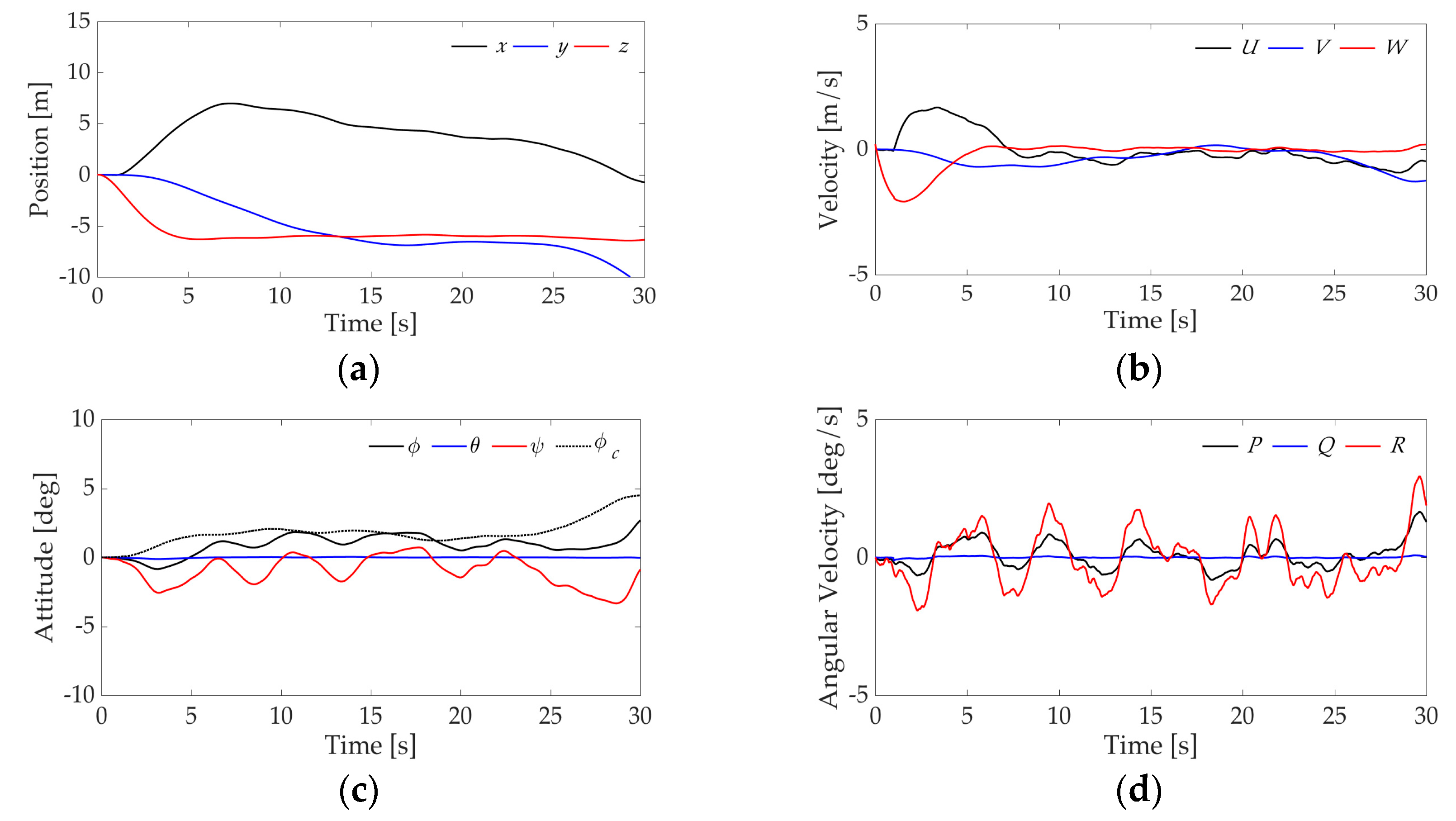
Figure 11 and Figure 12 show the results of numerical simulation without use of H-infinity controller and with use of the proposed controller, respectively. There is difference between commands of roll angles of both systems because those commands are calculated by using control input in translational motion of the UAV in Equation (30). It is revealed from Figure 11a,c that state variables of the UAV cannot reach those target values under the environment, whereas the proposed controller accomplish the control objective as shown in Figure 12a. However, it can be seen from these figures that control performance of lateral motion is deteriorated by wind disturbance.
Figure 11b,d shows that velocity and angular velocity change greatly, i.e., the disturbance has a significant influence on the state variables. On the other hand, Figure 12b,d shows that the variation in velocity and angular velocity is suppressed by using the proposed method. These results show that the proposed controller is useful under the wind disturbance in comparison with the conventional controller.
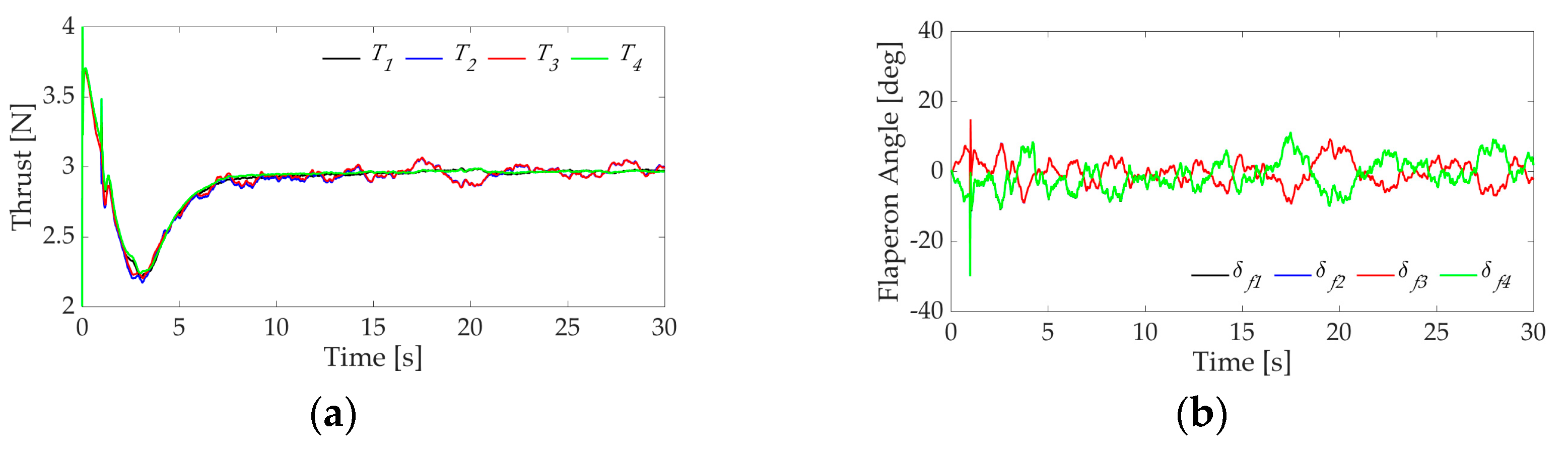
Figure 13 and Figure 14 show time histories of control inputs in both controllers. Although small vibration with high frequency can be seen in Figure 14 in comparison with results of the conventional system shown in Figure 13, the proposed controller satisfies constraints of control inputs shown in Table 3.
5. Experiment
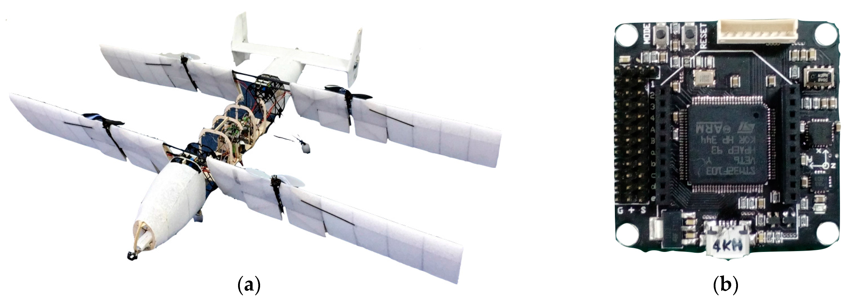
We developed a QTW-UAV to perform a preliminary experiment. Figure 15a shows the overview of the developed QTW-UAV that is composed of expanded polypropylene (EPP), carbon fiber reinforced plastic (CFRP), and balsa wood. Specifications of the UAV are shown in Table 5. The UAV is equipped with a developed avionics system integrating a microcomputer, IMU, position sensor, radio module, and laser range finder (LRF), as shown in Figure 15b. The STM32F103 microcomputer, which houses a Cortex-M3 clocked at 72 MHz, was selected from STMicroelectronics (Geneva, Switzerland) as the main controller. The IMU comprises a 3-axis magnetometer, HMC5983 from Honeywell (Morristown, NJ, USA), a 3-axis accelerometer, and a 3-axis rate-gyro using the MPU-6000 series from InvenSense (San Jose, CA, USA). The Extended Kalman Filter (EKF) in the sensor fusion is used to estimate the state variables of the UAV. The position sensor, DW1000, is a distance measurement system using an Ultra Wideband (UWB) radio with an accuracy of 100 mm on the horizontal plane. The altitude of the UAV is obtained by a laser range finder with high accuracy. The communication device uses XBee (ZigBee: IEEE802.15.4) to transmit the state of the UAV to the PC. All of these devices are controlled by the microcomputer STM32F103 (STMicroelectronics) and perform the calculation of the controller at 50 Hz. The system diagram is shown in Figure 16.
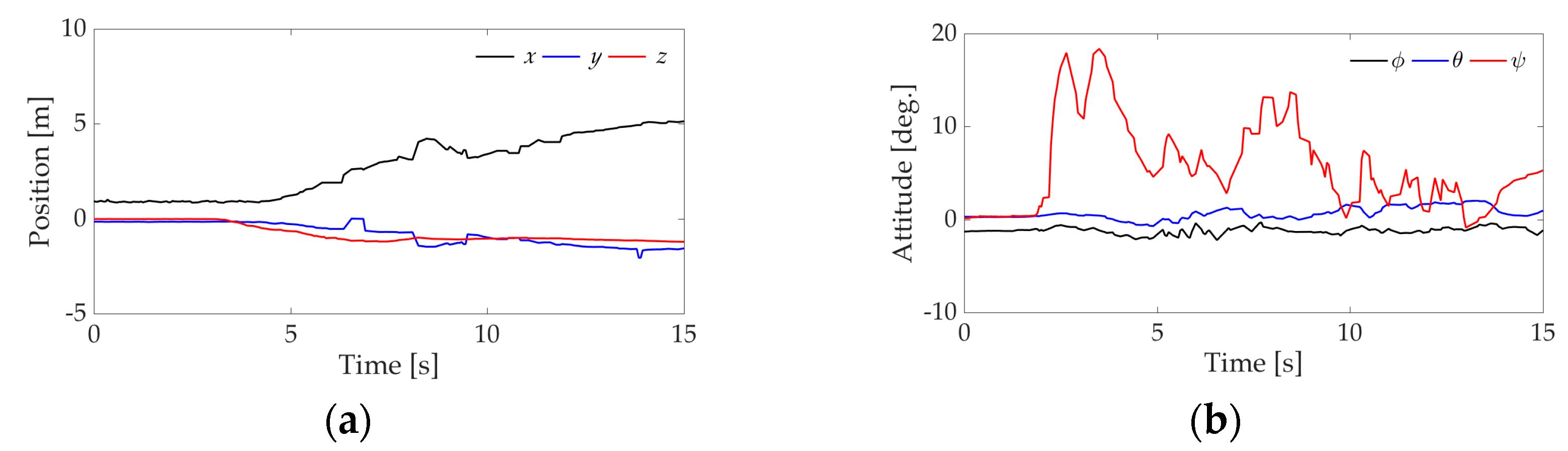
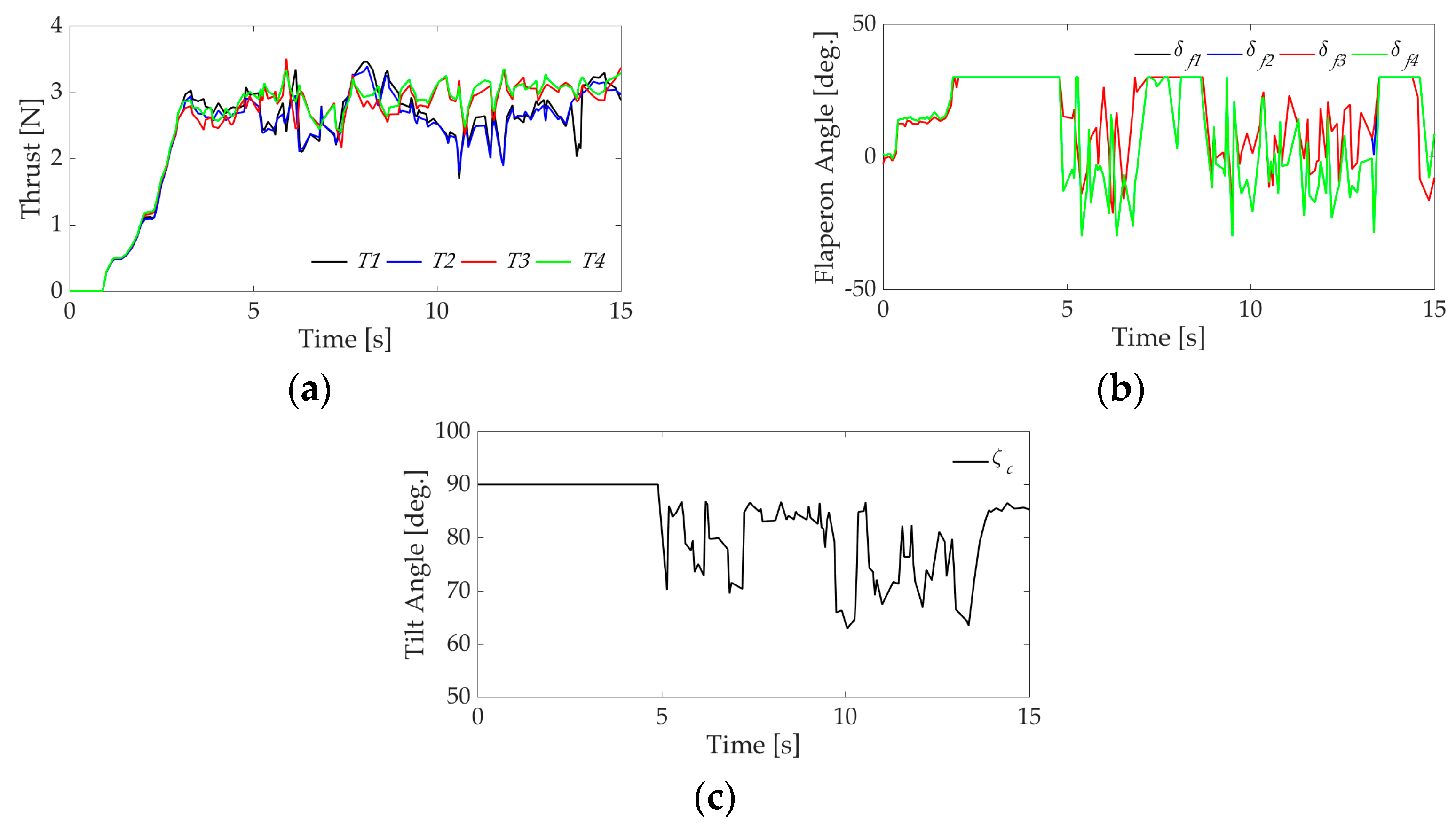
We conducted an experiment of transition flight of the QTW-UAV with the condition shown in Table 6. Figure 17 shows time histories of state variables, and Figure 18 shows time histories of control inputs. It is clear from the figure that the UAV is controlled stably during the transition flight even though there are small errors with respect to the attitude of the UAV. Good results similar to the numerical simulation are obtained by using the proposed flight control system. However, the steady-state errors of translational motion are recognized in Figure 17a due to disturbance such as side wind even though the position is obtained from the sensor with high accuracy. The result shows that the robustness of designed LQ controller for the translational motion is insufficient under the experimental condition. It is noted that H-infinity controller should be applied to translational motion of the UAV to compensate robust performance under wind environment.
6. Conclusions
We proposed a flight control system for a QTW-UAV considering its nonlinear dynamics and disturbances. In particular, the designed controller compensates disturbances such as modeling error and gusts by using H-infinity control theory. An observer based on the DAC method was used to estimate the nonlinear term including aerodynamic forces and moments of force. Numerical and experimental results showed the validity of the proposed flight control system. In the future, we will apply an H-infinity controller to translational motion and propose a more robust control system against disturbances such as gusts.
Author Contributions
The research objectives were developed between the authors. Numerical simulation and experiments were conducted by Kai Masuda with guidance and opinions from Kenji Uchiyama.
Conflicts of Interest
The authors declare no conflict of interest.
Nomenclature
| Position | |
| attitude angle (roll, pitch, and yaw) | |
| angle of attack | |
| velocity in the body coordinate system | |
| angular velocity in the body coordinate system | |
| mass of the QTW-UAV | |
| gravitational acceleration | |
| air density | |
| inertia tensor | |
| inertia of propeller | |
| distance between center of gravity and actuator | |
| distance between rotational axis of wing and application of thrust generated by flaperon | |
| diameter of propeller | |
| wing area | |
| representative area of body | |
| wing area of flaperon | |
| wing area of vertical stabilizer | |
| area of rotating surface of propeller | |
| lift coefficient of wing | |
| drag coefficient of wing | |
| lift coefficient of body | |
| drag coefficient of body | |
| coefficient of thrust | |
| coefficient of vertical stabilizer | |
| lift coefficient of propeller | |
| drag coefficient of propeller | |
| dynamic pressure for each wing | |
| dynamic pressure generated by propeller slipstream | |
| velocity of propeller slipstream | |
| angular velocity of propeller | |
| anti-torque of propeller | |
| propeller thrust | |
| flaperon angle | |
| tilt angle | |
| transformation matrix from inertial coordinate system to body coordinate system using Euler angle | |
| transformation matrix from body coordinate system to inertial coordinate system using Euler angle | |
| transformation matrix relating to Euler angle | |
| Subscript | |
| command value |
References
- Cox, T.H.; Nagy, C.J.; Skoog, M.A.; Somers, I.A. Civil UAV Capability Assessment Draft Version; NASA Report; NASA: Washington, DC, USA, 2004.
- Puri, A. A Survey of Unmanned Aerial Vehicles (UAV) for Traffic Surveillance; Department of Computer Science and Engineering, University of South Florida: Tampa, FL, USA, 2008. [Google Scholar]
- Kokume, M.; Uchiyama, K. Control Architecture for Transition between Level Flight to Hovering of a Fixed-Wing UAV. J. JSASS 2012, 60, 173–180. [Google Scholar] [CrossRef]
- Schoellig, A.; Augugliaro, F.; Lupashin, S.; D’Andrea, R. Synchronizing the Motion of a Quadrocopter to Music. In Proceedings of the IEEE International Conference on Robotics and Automation, Anchorage, AK, USA, 3–7 May 2010; pp. 3355–3360. [Google Scholar]
- Lupashin, S.; Schoellig, A.; Sherback, M.; D’Andrea, R. A Simple Learning Strategy for High-Speed Quadrocopter Multi-Flips. In Proceedings of the IEEE International Conference on Robotics and Automation, Anchorage, AK, USA, 3–7 May 2010; pp. 1642–1648. [Google Scholar]
- Nonami, K. Prospect and Recent Research & Development for Civil Use Autonomous Unmanned Aircraft as UAV and MAV. J. Syst. Des. Dyn. 2007, 1, 120–128. [Google Scholar]
- Kimura, G.; Furuya, M.; Yasuda, K.; Hirabayashi, D. Transportation System of QTW (Quad Tilt Wing)-UAV (Unmanned Aerial Vehicle). Trans. Logist. Conf. 2007, 16, 121–122. [Google Scholar]
- Sato, M.; Muraoka, K. Flight Test Verification of Flight Controller for Quad Tilt Wing Unmanned Aerial Vehicle. In Proceedings of the AIAA Guidance, Navigation, and Control (GNC) Conference, Boston, MA, USA, 19–22 August 2013. [Google Scholar]
- Sato, M.; Muraoka, K. Flight Control of Quad Tilt Wing Unmanned Aerial Vehicle. J. JSASS 2013, 61, 110–118. [Google Scholar] [CrossRef]
- Cetinsoy, E.; Dikyar, S.; Hancer, C.; Oner, K.T.; Sirimoglu, E.; Unel, M.; Aksit, M.F. Design and Construction of a Novel Quad Tilt-Wing UAV. Mechatronics 2012, 22, 723–745. [Google Scholar] [CrossRef]
- Hancer, C.; Oner, K.T.; Sirimoglu, E.; Cetinsoy, E.; Unel, M. Robust hovering control of a Quad Tilt-Wing UAV. In Proceedings of the 36th Annual Conference on IEEE Industrial Electronics Society (IECON 2010), Glendale, AZ, USA, 7–10 November 2010. [Google Scholar]
- Tran, A.T.; Sakamoto, N.; Sato, M.; Muraoka, K. Control Augmentation System Design for Quad-Tilt-Wing Unmanned Aerial Vehicle via Robust Output Regulation Method. IEEE Trans. Aerosp. Electron. Syst. 2017, 53, 357–369. [Google Scholar] [CrossRef]
- Hirata, Y.; Uchiyama, K. Transition Flight Control of QTW-UAV with Nonlinear Parameter—Varying Model. In Proceedings of the 53th Aircraft Symposium, Ehime, Japan, 11–13 November 2015. (In Japanese). [Google Scholar]
- Mikami, T.; Uchiyama, K. Design of Flight Control System for Quad Tilt-Wing UAV. In Proceedings of the 2015 International Conference on Unmanned Aircraft Systems, Denver, CO, USA, 9–12 June 2015. [Google Scholar]
- Johnson, C.D. A Family of ”Universal Adaptive Controllers” for Linear and Nonlinear Plants. In Proceedings of the Twentieth Southeastern Symposium on System Theory, Charlotte, NC, USA, 20–22 March 1988; pp. 530–534. [Google Scholar]
- Akai, Y.; Shimada, Y.; Uchiyama, K.; Abe, A. Design for Nonlinear Attitude Control System for Spaceplane Using Disturbance-Accommondating Control. Proc. KASAS-JSASS Jt. Int. Symp. Aerosp. Eng. 2008, 11, 542–547. [Google Scholar]
- Flying Qualities of Piloted Airplanes; U.S. Military Specification MIL-F-8785C; U.S. Department of Defense: Washington, DC, USA, 1980.
Figure 1.
Flight configuration.
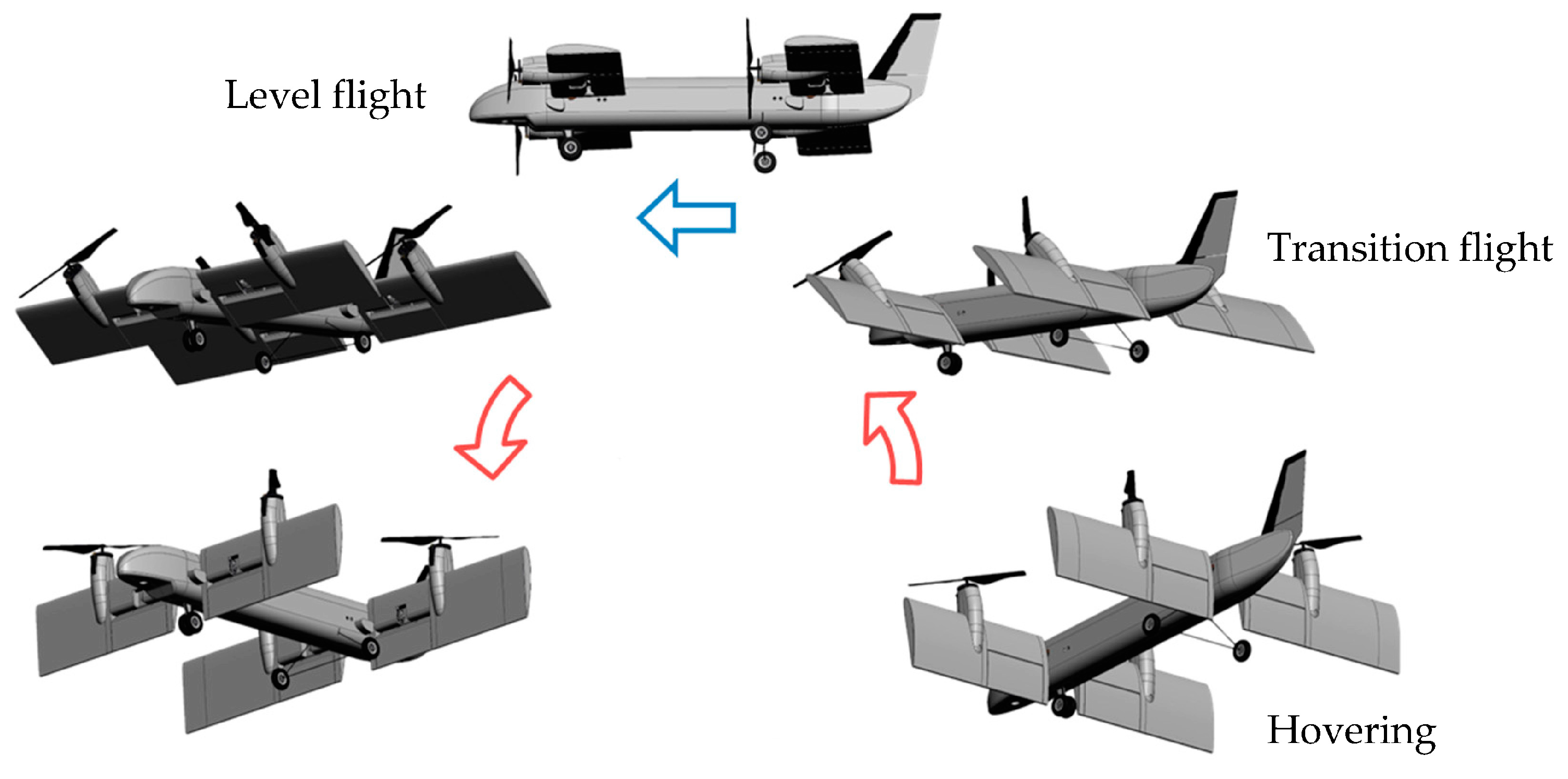
Figure 2.
Definition of state variables and control inputs.
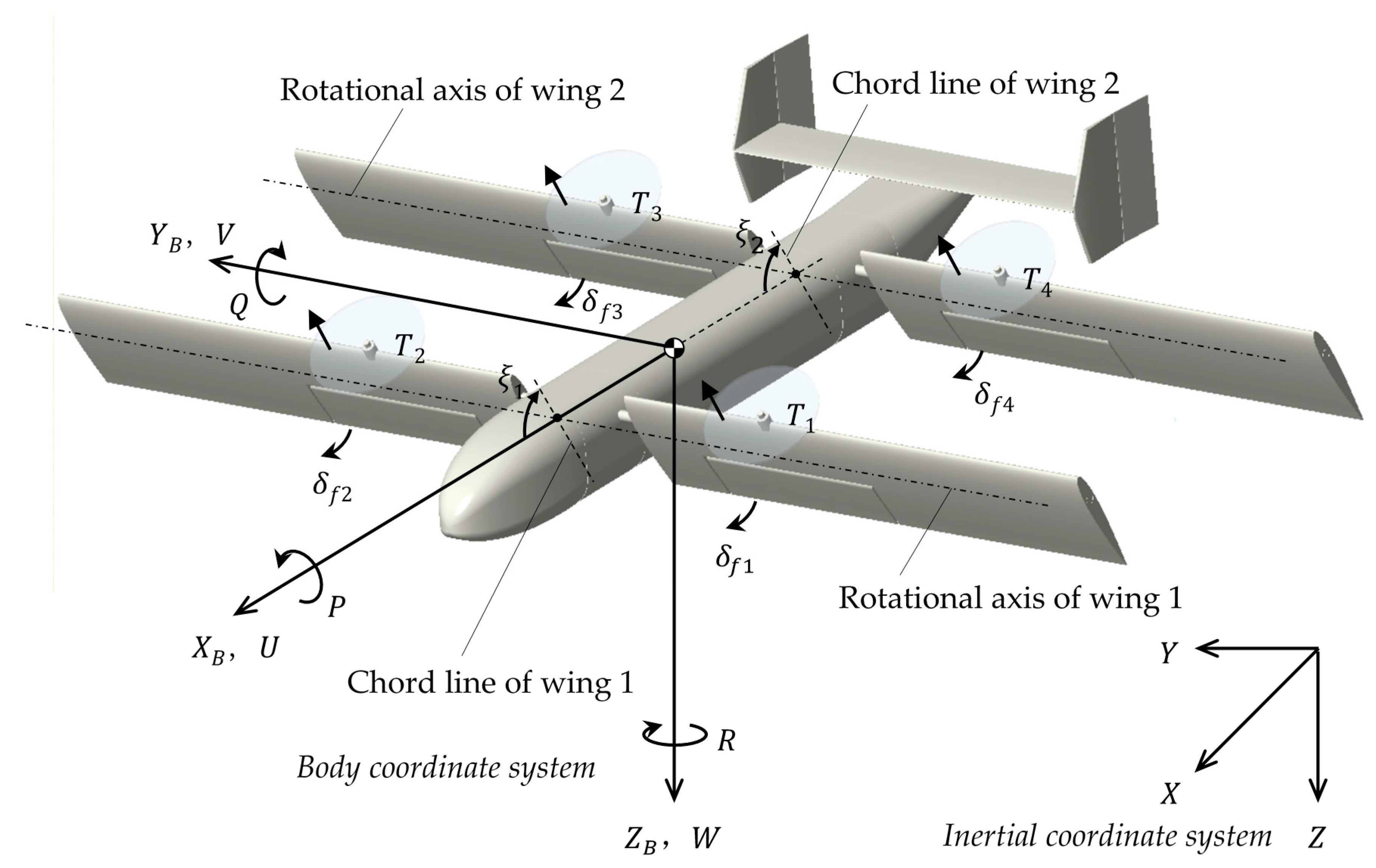
Figure 3.
Arrangement of the propeller and flaperon.

Figure 4.
Block diagram of proposed flight control system.
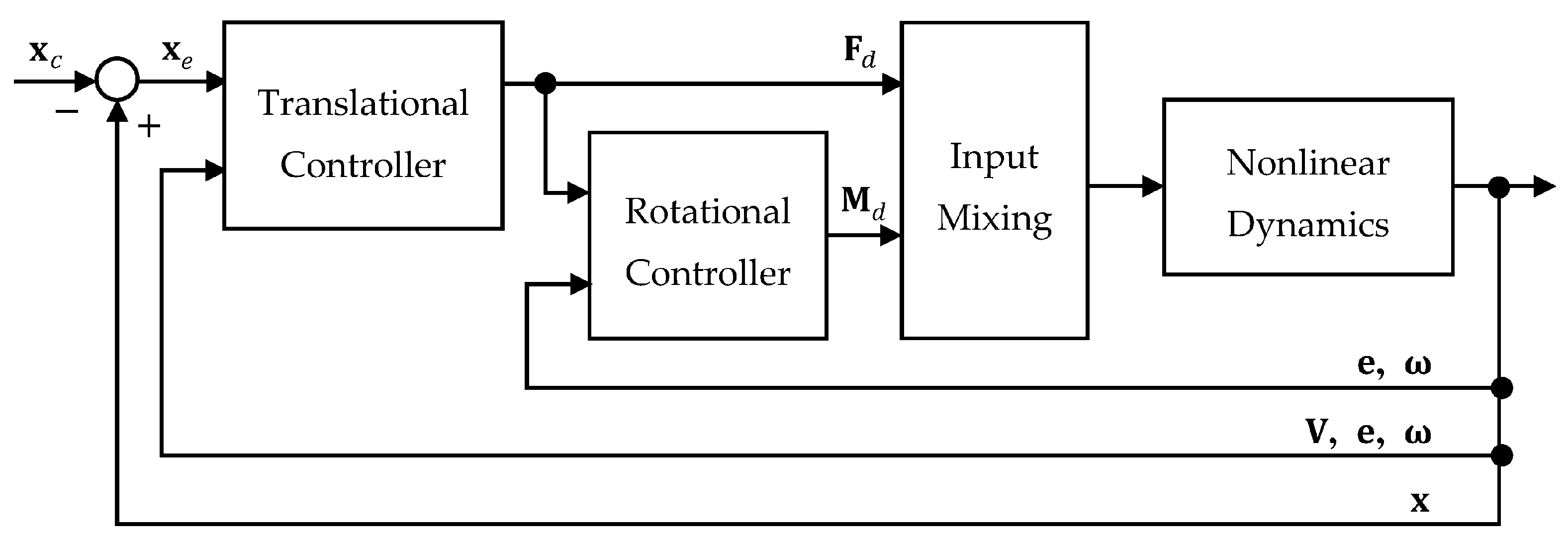
Figure 5.
Block diagram of proposed translational control system.
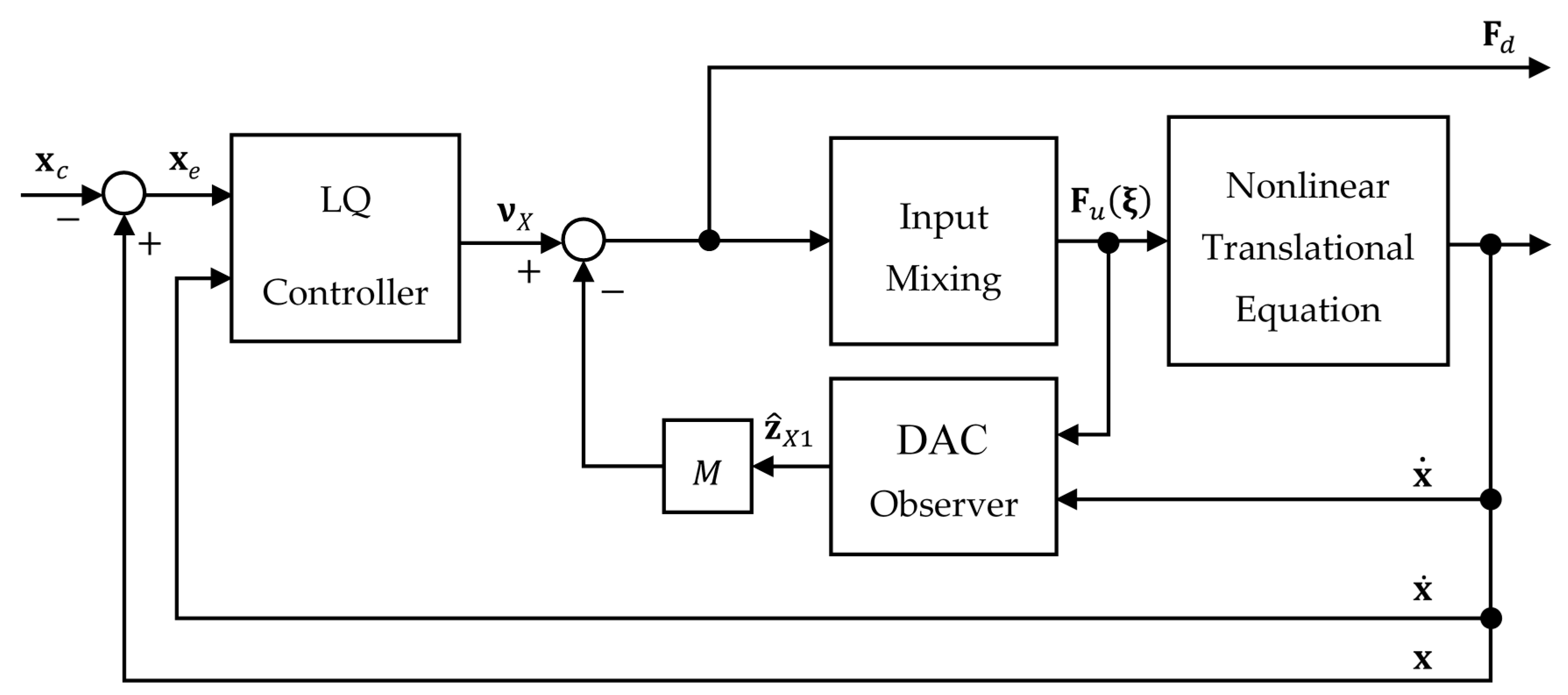
Figure 6.
Definition of command angle.
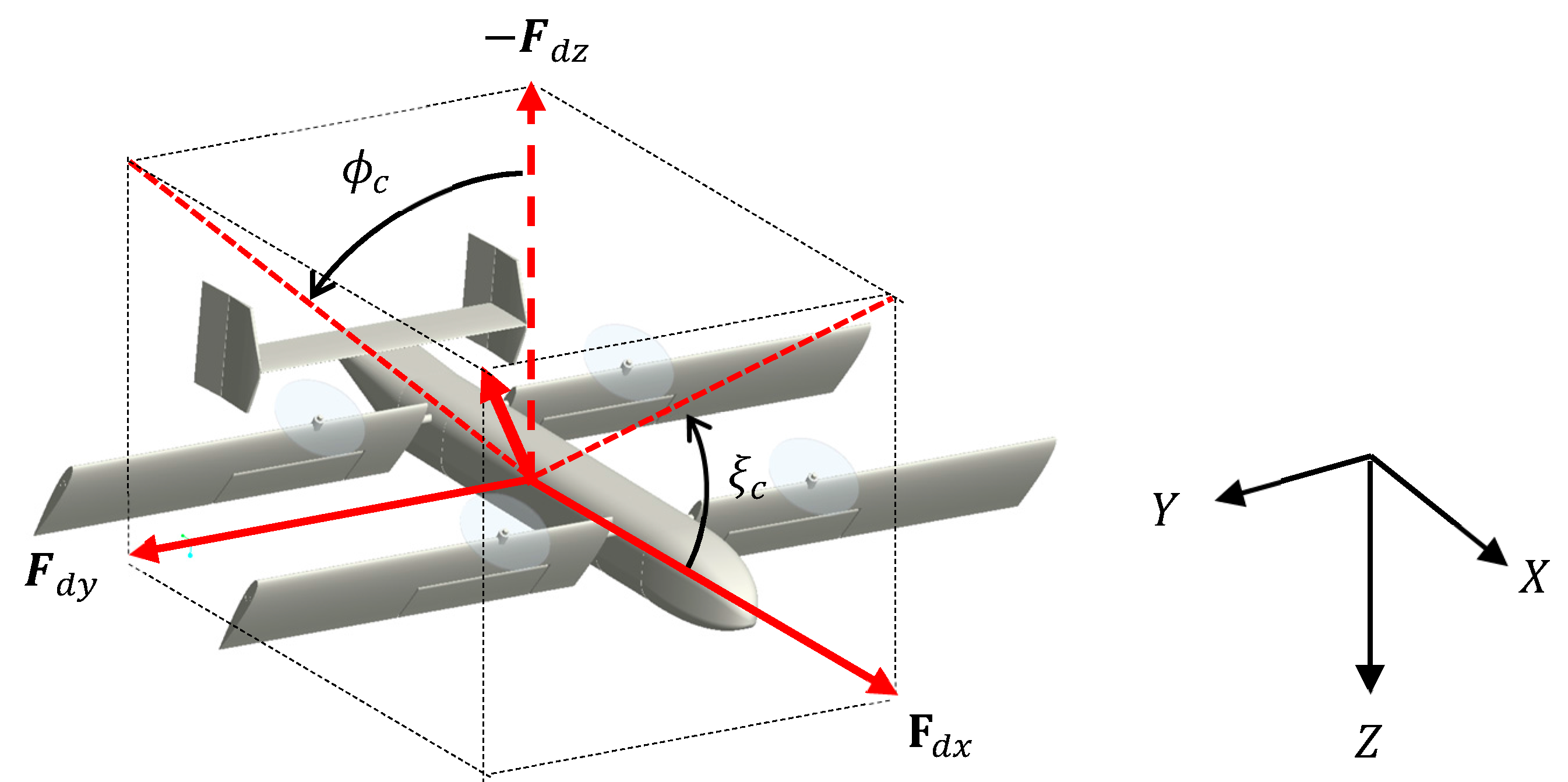
Figure 7.
Generalized plant.

Figure 8.
Block diagram of proposed rotational control system.

Figure 9.
Definition of actuator coordinate system.

Figure 10.
Dynamic characteristics of control system in frequency domain.
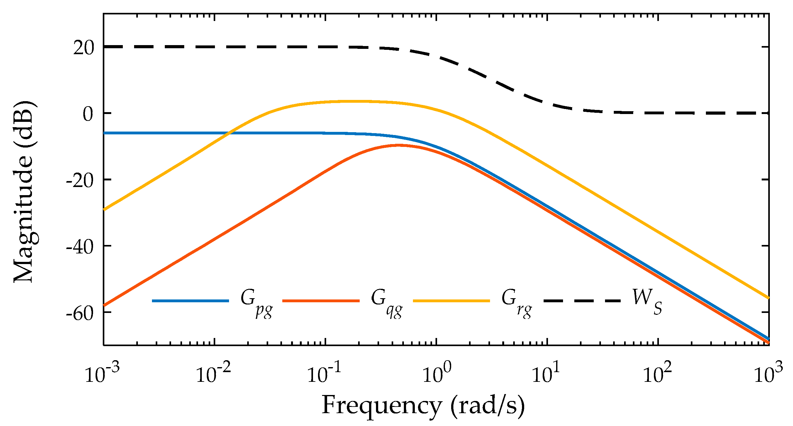
Figure 11.
Time responses of state variables using conventional controller. (a) Position; (b) Velocity; (c) Attitude; (d) Angular velocity.
Figure 11.
Time responses of state variables using conventional controller. (a) Position; (b) Velocity; (c) Attitude; (d) Angular velocity.

Figure 12.
Time responses of state variables using proposed controller. (a) Position; (b) Velocity; (c) Attitude; (d) Angular velocity.
Figure 12.
Time responses of state variables using proposed controller. (a) Position; (b) Velocity; (c) Attitude; (d) Angular velocity.
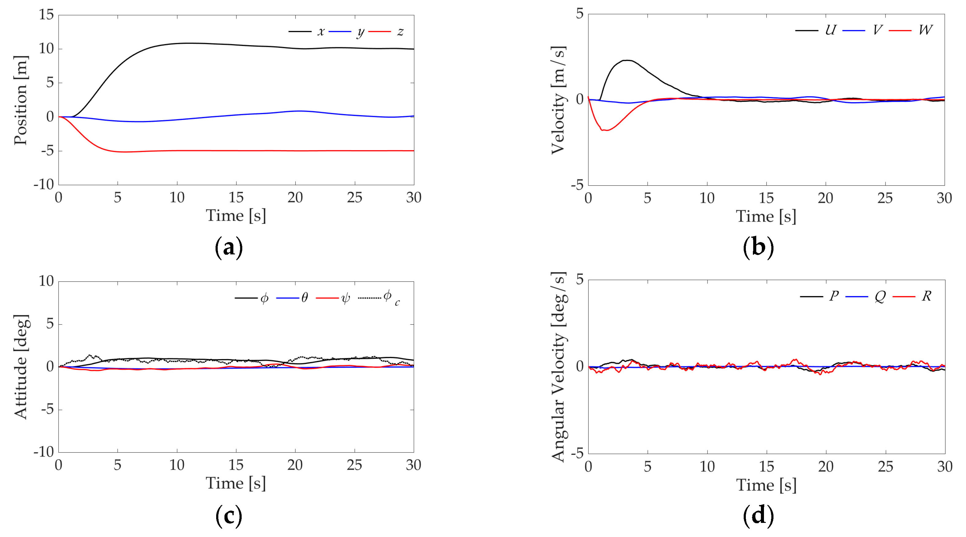
Figure 13.
Time responses of control inputs using conventional controller. (a) Thrust; (b) Flaperon angle; (c) Tilt angle.
Figure 13.
Time responses of control inputs using conventional controller. (a) Thrust; (b) Flaperon angle; (c) Tilt angle.
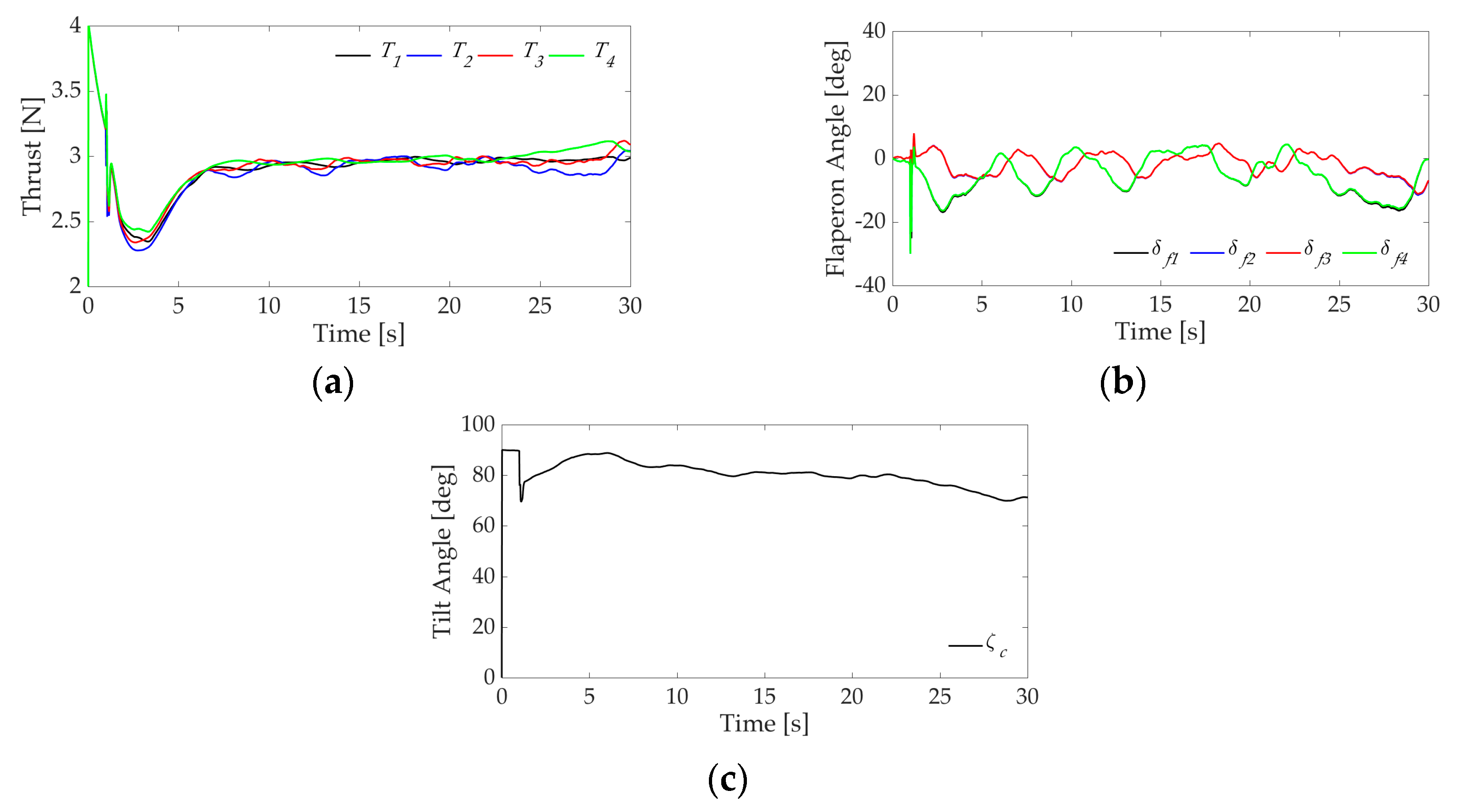
Figure 14.
Time responses of control inputs using proposed controller. (a) Thrust; (b) Flaperon angle; (c) Tilt angle.
Figure 14.
Time responses of control inputs using proposed controller. (a) Thrust; (b) Flaperon angle; (c) Tilt angle.

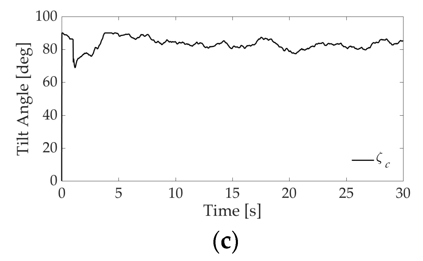
Figure 15.
Developed (a) QTW-UAV and (b) avionics.

Figure 16.
System diagram.
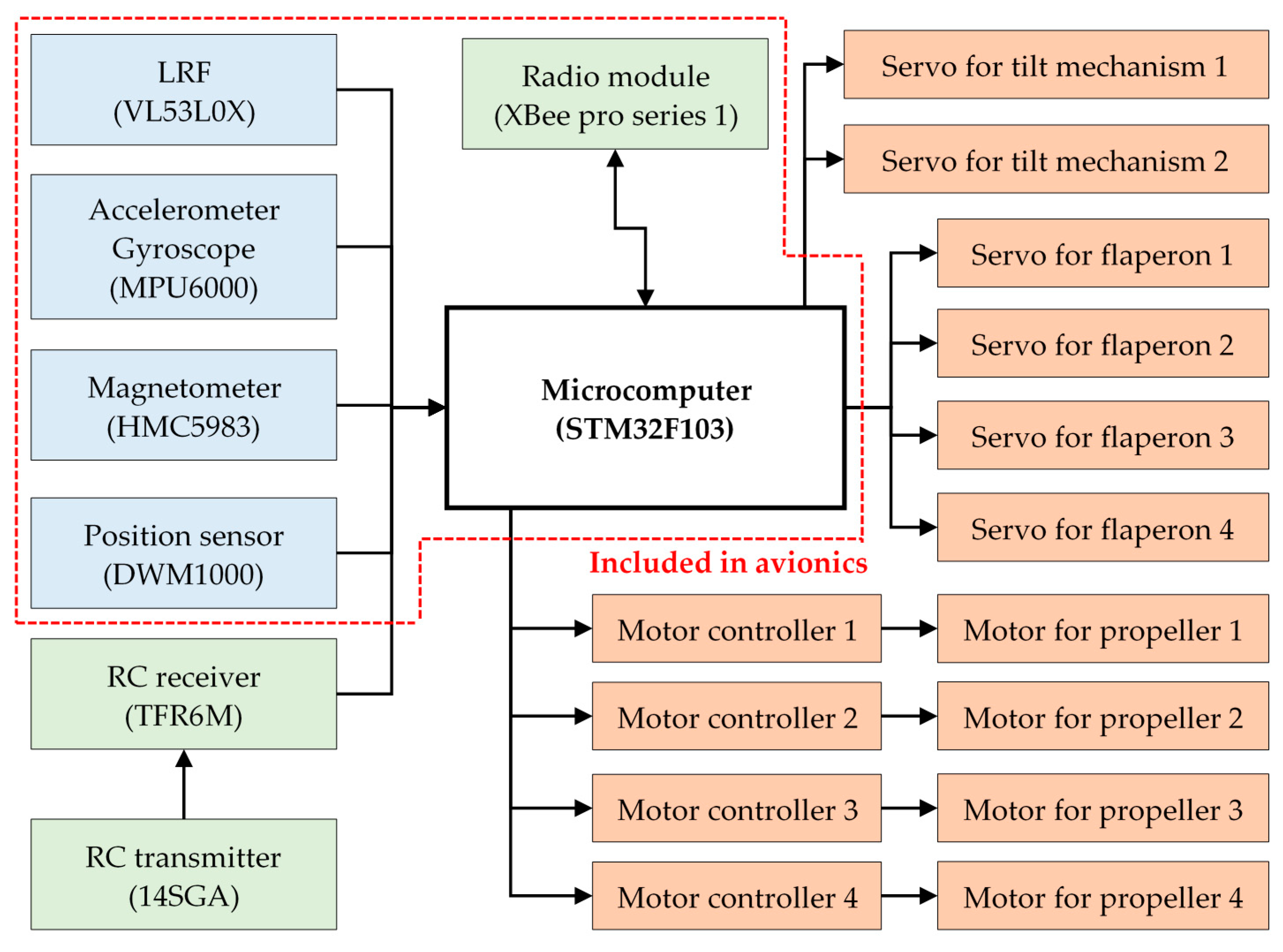
Figure 17.
Experimental result of (a) position, (b) attitude and (c) angular velocity using proposed controller.
Figure 17.
Experimental result of (a) position, (b) attitude and (c) angular velocity using proposed controller.

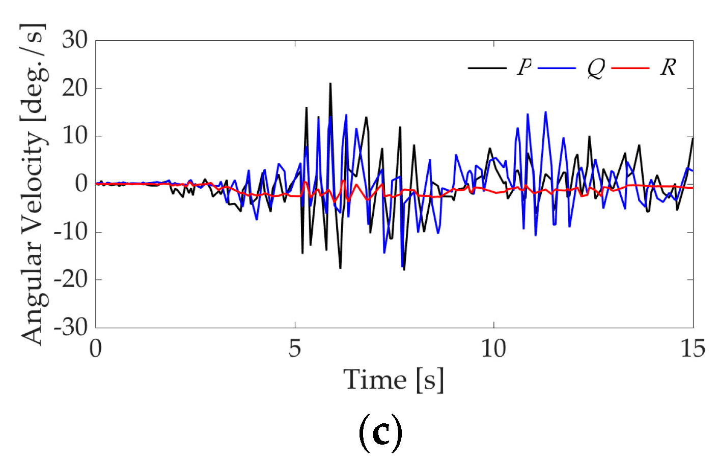
Figure 18.
Experimental result of (a) thrust, (b) flaperon angle and (c) tilt angle using proposed controller.
Figure 18.
Experimental result of (a) thrust, (b) flaperon angle and (c) tilt angle using proposed controller.


Table 1.
System configuration.
| Type of System | Translational Motion | Rotational Motion |
|---|---|---|
| Proposed controller | LQ controller DAC observer | H-infinty controller DAC observer |
| Conventional controller | LQ controller | LQ controller |
Table 2.
Parameters.
| Parameter | Value | Unit | Parameter | Value | Unit |
|---|---|---|---|---|---|
Table 3.
Constraints of actuator.
| Variable | Range | Unit | |
|---|---|---|---|
| propeller thrust | |||
| Flaperon angle | |||
| Tilt angle | |||
Table 4.
Initial condition and target values.
| Parameter | Value | Unit | ||
|---|---|---|---|---|
| Position | ||||
| Velocity | ||||
| Attitude | ||||
| Angular velocity | ||||
| Target position | ||||
| Target attitude | ||||
Table 5.
Specification of the Quad Tilt-Wing Unmanned Aerial Vehicle (QTW-UAV).
| Parameter | Value | Unit | |
|---|---|---|---|
| Mass | |||
| Total height | |||
| Overall length | |||
| Span of front wing | |||
| Span of rear wing | |||
Table 6.
Initial condition and target values in experiment.
| Parameter | Value | Unit | ||
|---|---|---|---|---|
| Position | ||||
| Velocity | ||||
| Attitude | ||||
| Angular velocity | ||||
| Target position | ||||
© 2018 by the authors. Licensee MDPI, Basel, Switzerland. This article is an open access article distributed under the terms and conditions of the Creative Commons Attribution (CC BY) license (http://creativecommons.org/licenses/by/4.0/).
Share and Cite
MDPI and ACS Style
Masuda, K.; Uchiyama, K. Robust Control Design for Quad Tilt-Wing UAV. Aerospace 2018, 5, 17. https://doi.org/10.3390/aerospace5010017
AMA Style
Masuda K, Uchiyama K. Robust Control Design for Quad Tilt-Wing UAV. Aerospace. 2018; 5(1):17. https://doi.org/10.3390/aerospace5010017
Chicago/Turabian StyleMasuda, Kai, and Kenji Uchiyama. 2018. "Robust Control Design for Quad Tilt-Wing UAV" Aerospace 5, no. 1: 17. https://doi.org/10.3390/aerospace5010017
Note that from the first issue of 2016, this journal uses article numbers instead of page numbers. See further details here.