Robust Autoland Design by Multi-Model ℋ∞ Synthesis with a Focus on the Flare Phase

Systems & Information Processing Department, The French Aerospace Lab (ONERA), 31055 Toulouse, France
*
Author to whom correspondence should be addressed.
Aerospace 2018, 5(1), 18; https://doi.org/10.3390/aerospace5010018
Submission received: 29 November 2017
/
Revised: 26 January 2018
/
Accepted: 7 February 2018
/
Published: 9 February 2018
(This article belongs to the Special Issue Aircraft Dynamics & Control)
Abstract
:Recent advances in the resolution of multi-model and multi-objective control problems via non-smooth optimization are exploited to provide a novel methodology in the challenging context of autoland design. Based on the structured control framework, this paper focuses on the demanding flare phase under strong wind conditions and parametric uncertainties. More precisely, the objective is to control the vertical speed of the aircraft before touchdown while minimizing the impact of windshear, ground effects, and airspeed variations. The latter is indeed no longer controlled accurately during flare and strongly affected by wind. In addition, parametric uncertainties are to be considered when designing the control laws. To this purpose, extending previous results published by the authors in a conference paper, a specific multi-model strategy taking into account variations of mass and center-of-gravity location is considered. The methodology is illustrated on a realistic aircraft benchmark proposed by the authors, which is fully described in this paper and freely available from the SMAC (Systems Modeling Analysis & Control) toolbox website (http://w3.onera.fr/smac).
1. Introduction
The steady growth of air traffic in recent years has led to drastic safety standards with the goal of limiting the number of accidents. Since approach and landing remain the most critical flight phases (almost 50% of fatal accidents and 75% of non-fatal hull losses between 1997 and 2016 [1]), particular attention has recently focused on improving autoland systems in adverse conditions. With the help of CAT III instrument landing systems (ILS), which are now available in a rapidly growing list of airports, automatic landing control laws have helped to secure these two phases notably in degraded weather conditions (such as fog and crosswinds). However, despite numerous methodological works [2,3,4,5] over the past two decades, the design, tuning, and validation process of final approach and flare control systems remains a challenging and time-consuming task. As is observed in [4], where a complete design framework together with a dedicated software is proposed, the tuning phase requires rather tricky multi-objective optimization. Note, however, that optimizing the parameters of the flare control system (such as initial altitude and vertical velocity profile) becomes much easier when the internal loops are correctly designed and tuned. In our context, a natural choice is to track the vertical velocity. The main difficulty is to obtain fast and accurate responses despite a significant airspeed decrease, possible windshear, and ground effects. Recall indeed that the flare segment generally lasts less than s and that, to ensure good robust performance properties, the desired vertical speed should be reached at least 1 or s before touchdown. Unlike the approaches detailed in [4,6,7], either using robust nonlinear dynamic inversion or adaptive control schemes to design the aforementioned inner loops, linear-oriented techniques are often preferred by a majority of contributions. It can be observed indeed that, during approach and landing, airspeed and altitude variations remain rather small so that the aircraft behavior is almost linear. In the field of flight control design, the most popular methods are still based today on eigenstructure assignment [8] or LQR (Linear Quadratic Regulator) control techniques [5]. Both approaches have been successfully used in Airbus and Boeing design offices and have contributed for nearly 30 years to considerable improvements in the flight control design process. In the meantime, control techniques have been progressively developed and evaluated on various flight control problems—see, for example, [2,3], where the flare phase receives particular attention. Yet, despite promising results even in flight tests [9], this third approach has not become as popular as the other two in the industry. Things are, however, likely to change in the near future with the emergence of new tools based on non-smooth optimization techniques [10,11]. With these approaches, it becomes possible to impose constraints on the structure and the order of the controller. Although convexity is unfortunately lost in that case, the aforementioned algorithms converge to local solutions, which are (in a large majority of standard applications) not so far from the global (non-structured) optimum. Another interesting feature of these new tools is their capacity to handle multiple models and multiple separate channels [12]. This last feature offers new ways to define design models, which will be used in this paper to solve the flare control problem despite modeling errors and parametric uncertainties, thus extending the results of [13].
The paper is organized as follows. ILS-based automatic landing issues are briefly reviewed in Section 2. The flare control problem is then detailed and solved by a multi-model and multi-channel design approach in Section 3. Specific attention is devoted in this section to robustness. Implementation issues and nonlinear simulation results are then presented in Section 4. Finally, Section 5 concludes the paper and details a few perspectives. For the sake of completeness, a thorough description of the aircraft model used in the nonlinear simulations is presented in Appendix A. This aircraft model together with a complete description of the design problem is freely available from the SMAC toolbox (dedicated to Systems Modeling, Analysis and Control) website (http://w3.onera.fr/smac).
2. ILS-Based Automatic Landing
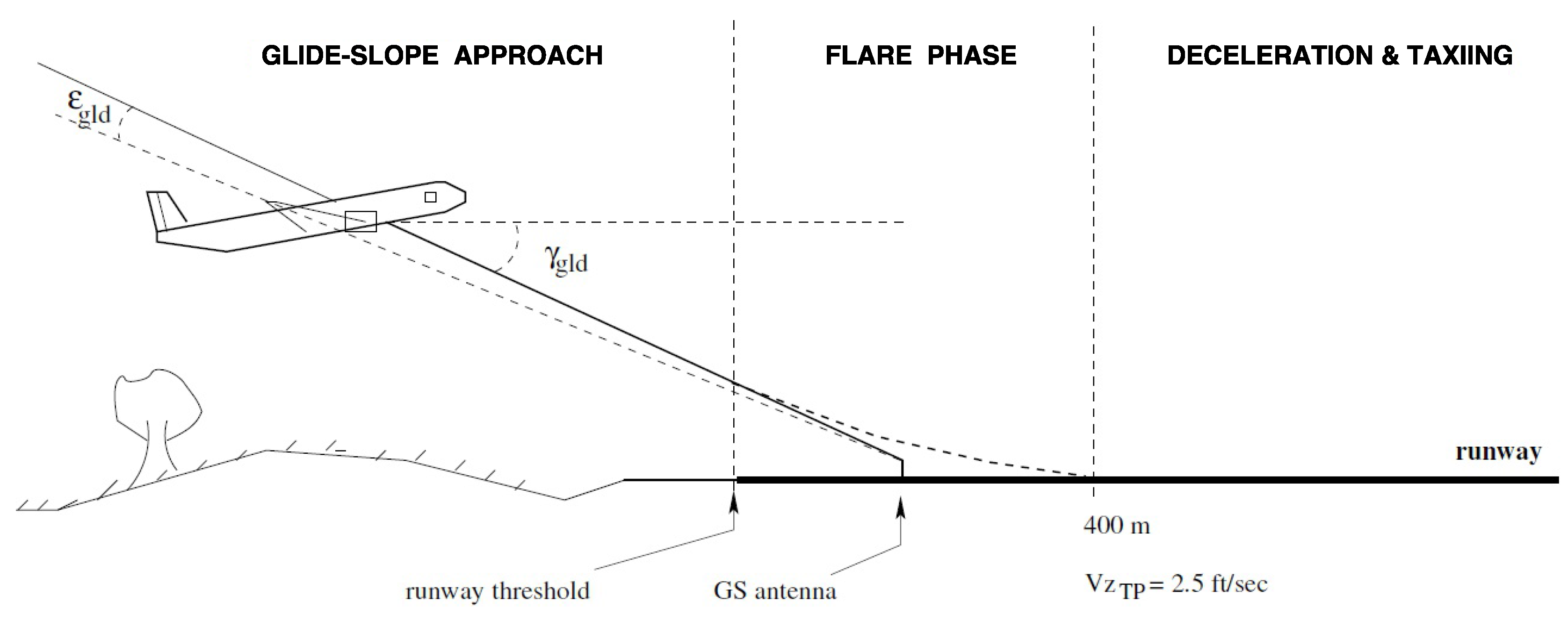
As illustrated in Figure 1, automatic landing in the vertical plane can be divided into two main phases: the final approach during which the aircraft must follow a descent path (glide) and the flare segment, which is activated when the landing gear height falls below a threshold value . The latter is most often fixed around ft but might be slightly updated as a function of ground speed. Similarly, in the horizontal plane, the aircraft trajectory must coincide with the runway axis (localizer phase) as long as ft. The alignment phase (or decrab mode) is then activated in order to minimize the lateral efforts on the landing gears at touchdown.
Automatic landing control systems are generally designed on simplified models, using decoupling hypotheses between the longitudinal and the lateral axes. These assumptions, particularly during the landing phase, are usually satisfied without any severe restriction for a large majority of civil and military aircraft.
2.1. Final Approach
During the final approach, as already clarified, the trajectory of the aircraft must be kept as close as possible to the ILS beam. This is achieved by simultaneously minimizing the norm of the longitudinal and lateral errors and , where is the angular error between the nominal glide path and that of the aircraft (see Figure 1), and denotes the lateral angular error in the horizontal plane. In both cases, and are elementary altitude-dependent arctangent-based nonlinear functions that convert angular errors into metric deviations.
Moreover, during this phase, the calibrated airspeed is to be kept constant, and the aerodynamic sideslip angle must remain zero. Based on the decoupling assumption and the above constraints, most autoland systems are usually based on two inner control loops. In this paper, the following structures are used for the longitudinal and the lateral axis, respectively:
where , , , p, q, r, denote the vertical speed, the longitudinal and lateral load factors, the roll, the pitch and yaw rates, and the bank angle, respectively. , , , are the control inputs (thrust and elevator/aileron/rudder deflections), while the subscript c stands for a commanded value. The static gains and are tuned on linearized models by a standard eigenstructure assigment method. The eigenvectors are constrained so as to ensure decoupling between and along the longitudinal axis and between and along the lateral axis. Note the use of small letters in Equation (1) to denote the longitudinal and the vertical speeds, which correspond here to variations about their nominal or initial values. This notation will further be used in the remaining of the paper.
Thus, the outer control loops are easily tuned. Observing that , a fairly standard proportional controller can be used to ensure a nominal trajectory in the vertical plane, while the commanded variations on the calibrated airspeed are simply set to 0:
Next, using a bank-to-turn strategy, the lateral deviation is controlled via a proportional-derivative action on the bank angle. Finally, the sideslip angle, which is not directly measured, is controlled via the lateral load factor:
Remark 1.
The derivative term is not directly accessible to the control law and a pseudo-derivation of would introduce a very high noise level since is highly affected by noise as well. Then, the following approximation can be used:
where χ and denote the route angle and the ground speed, respectively.
2.2. Flare and Align Phases
The nominal slope during approach is generally fixed to deg, and the airspeed is a function of mass and mean wind. For the considered aircraft, whose mass belongs to the interval , the nominal approach airspeed is around . The vertical speed then remains above during this phase but should fall below before touchdown. The flare phase, which starts at approximately above ground and generally lasts less than s, is then essential for reducing the vertical speed as fast as possible from to less than . To achieve this goal, the simplest strategy is to update in the longitudinal outer control loop (Equation (3)). Unfortunately, the inner control loop (Equation (1)) is generally much too slow. Moreover, the airspeed can no longer be controlled accurately during this phase and the throttle must be reduced to idle. A completely new design, to be further detailed in Section 3, is then required.
Initiated ft above ground, the objective of the align phase is to make sure that the longitudinal axis of the plane coincides with that of the runway at touchdown. This is simply realized by relaxing the constraint on the aerodynamic sideslip angle. Thus, the outer-loop is simply replaced by
where denotes the heading angle error to be reduced to 0. The parameter is generally tuned empirically until the decrab objectives are met.
2.3. Overview of the Autoland Architecture
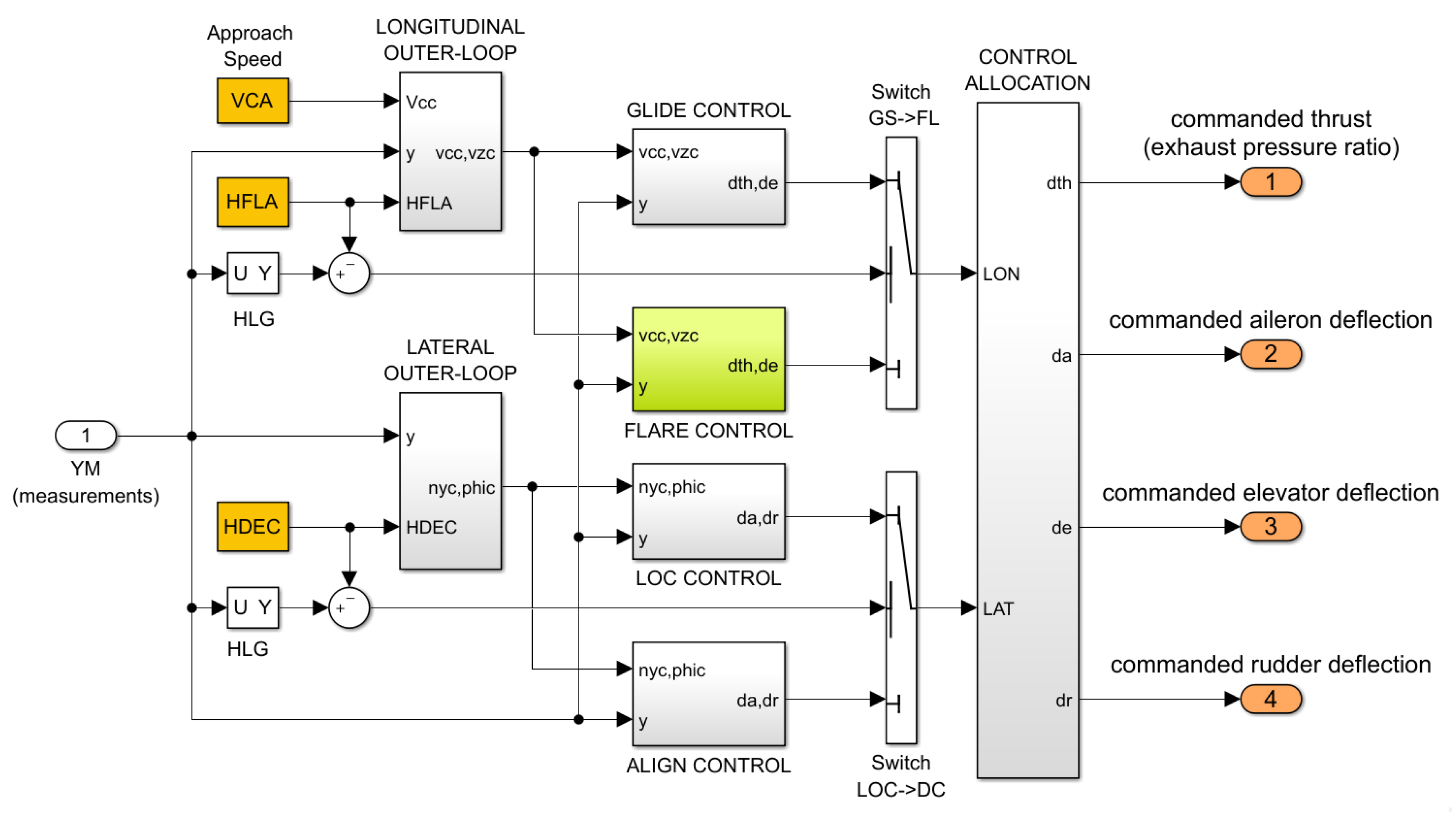
The above four elements consisting of glide, localizer, flare, and alignment control subsystems are now assembled as shown in Figure 2 to define the global autoland system.
These four subsystems are coordinated by two decoupled longitudinal and lateral outer-loops, which, respectively, deliver the desired signals to be followed on each axis ( for the longitudinal axis and for the lateral axis). Note that these signals are adapted as a function of the landing gear height. Along the longitudinal axis, the desired vertical speed profile is modified when to ensure a soft landing while controlling the impact point. Simultaneously, the control loop gains and architecture are modified by switching from the glide to the flare control system. The same architecture is used along the lateral axis. When , the desired lateral acceleration is adapted to minimize the landing gear sideslip angle at touchdown despite crosswind. Simultaneously, the localizer tracking system is deactivated in favor of the alignment control device.
3. Flare Control Design
3.1. Overall Controller Structure
As briefly discussed above, the objective of the flare phase is to provide enhanced vertical speed control capacities so that the aircraft hits the runway about 400 m after threshold with a nominal vertical speed of ft/s. During this short maneuver, rarely exceeding s, the engines are set to the idle position and the airspeed is no longer accurately controlled (provided, of course that any stall risk is avoided). Along the longitudinal axis, the only remaining active control input is then the elevator deflection. As shown in Figure 3, the general structure of the flare system consists of two nested loops. A reference vertical speed profile is generated by the outer-loop. It depends on both the initialization altitude (generally close to 50 ft) and the ground speed. Despite perturbations and uncertainties, the generated profile should then be tracked accurately thanks to an appropriate tuning of the vertical speed inner-loop controller, whose design is described in the following section.
3.2. Vertical Speed Control via Multi-Channel Structured Optimization
The central objectives and constraints of the flare phase are fundamentally different from those encountered during the final approach. From a control viewpoint, the design problem appears to be simpler since only one variable (the vertical speed) is being tracked and only one control input (the elevator deflection) is being managed. However, the fluctuations of the (no longer controlled) longitudinal airspeed and the engine deceleration generate perturbations, which, in addition to the ground and wind effects, ultimately aggravate the control problem. It appears that modal control techniques (which have been successfully used to tune the glide controller) are no longer the best option to address this specific problem. The latter now falls within the scope of design methods.
The key issue is then to define an appropriate design model, which begins with the choice of relevant linear approximations of the aircraft longitudinal dynamics near the ground. Such models are easily obtained with trimming and linearization tools (available with the benchmark package as mentioned in Section A.6) for various points in the flare two-dimensional trajectory (height above runway and kinematic slope). After standard matrix manipulations of the state-space data, the following parameterized set of third-order models is considered:
where is the pitch angle, and denotes the height of the landing gear above ground (to alleviate notation, especially in Figure 4). Note that, in this model, and are no longer viewed as a state and a control input signal, respectively, but as external perturbations. However, unlike wind inputs , these are measured and can then be used for feedback. This is illustrated in the design diagram depicted in Figure 4. Note that the controller to be optimized reduces to a static gain . The proposed vertical speed control law structure then reads
where, as shown in the diagram, the signal coincides with the output of a linear reference model to be tracked. The main interest of the proposed structure is to remain close to the one used during the glide segment (see Equation (1)), which will not only simplify the switching strategy but also contribute to an improved safety level.
Let us now focus on the optimization criteria. Beyond the standard closed-loop stability requirements, the objective is to determine the best controller such that
- the norm of the error is minimized,
- the control activity is such that magnitude and rate saturations are avoided, and
- the perturbations have a negligible effect on the vertical speed variations.
In the framework [14], the first two objectives are realized through the norm minimization of the following transfer function (using the notation of Figure 4):
where denotes the parameterized (height-dependent) weighted standard interconnection from to , and stands for the lower linear fractional transformation (LFT). The weighting functions and are chosen following standard rules to be further discussed in Section 3.4. The third objective is then achieved by the norm minimization of an independent transfer from (with ) to :
where the three-dimensional filter is used to shape the input perturbations. However, as this transfer is considered independently of Equation (9), it is not restrictive to consider a static weighting function , where each static gain is used to scale the relative weights of each input perturbation. The three transfers then (Equation (10)) are weighted by a single scalar dynamic filter . In order to remove any static error (mostly induced by the speed variations) on , which could be critical near ground, a high-gain low-pass filter must be used.
Summarizing the above discussion, the controller optimization may now be stated as the following multi-model & multi-channel structured control design problem:
3.3. Robustness Against Parametric Uncertainties and Modeling Errors
By simultaneously considering several design models for different values of the height of the landing gear above ground, interesting robustness properties against ground effects modeling errors are enforced in the proposed design process. This is, however, not sufficient in practice, where parametric robustness against mass and center-of-gravity location is also required. To this end, the above multi-objective design framework is easily generalized to take these additional parametric uncertainties explicitly into account. Thus, the design problem (11) becomes
where the new integer indexes a selection of different models in the (mass × centering) hypercube. A common choice is to consider the vertices of the hypercube. Such a design may then be followed by an analysis phase in order to detect any potential worst-case that could appear inside the hypercube. An iterative design process described in [15] can therefore be considered by incorporating the worst-case scenarios into the initial selection of design models.
3.4. Weight Selection & Resolution Aspects
The above problems (Equations (11) and (12)) are strongly non-convex and cannot be solved with the standard control optimization tools, which provide unstructured full-order controllers and are unable to optimize separate channels on multiple models. However, using specialized non-smooth optimization techniques, some efficient algorithms have been proposed in [10] and then improved when they were implemented in the HINFSTRUCT and SYSTUNE routines of the Robust Control Toolbox [16].
In this application, the HINFSTRUCT routine was used on an augmented design model with a block-diagonal structure including models associated with
- two values of the landing gear height:
- four models (indexed by j) at the vertices of the (mass × centering) hypercube, and
- two separate optimization channels (indexed by i).
Despite potential numerical difficulties, for a given set of weighting functions, a solution is obtained in less than on a standard computer thanks to the efficiency of the specialized non-smooth optimization algorithm implemented in the HINFSTRUCT routine. Such a limited computational time allows for different trials in the selection of the weighting filters, which are detailed in the next section.
3.4.1. Reference Model on the Vertical Speed
To ensure good time response while remaining compatible with the aircraft dynamics, the reference model is chosen to be
where s, rad/s, and .
3.4.2. Performance & Robustness Oriented Weighting Filters
A low-pass filter (enforcing a high performance tracking of slowly varying inputs) is selected for while a high-pass filter (here approximated by a constant) is used for . After a short trial-and-error process, the weights are tuned as follows:
Note that a constant weighting function is sufficient in our context since the optimized controller is a static gain K. This may not be the case with dynamic controllers, for which roll-off properties generally have to be enforced via high-pass dynamic weighting functions.
Finally, as is already clarified in Section 3.2, static input weighting functions and a high gain low-pass output filter are tuned for the second channel, whose objective is to minimize the effects of perturbations (induced by airspeed, thrust, and wind variations) on the vertical speed:
3.4.3. Optimization Results
With the above filters, a worst-case norm is obtained around 1, and the following gains are computed:
4. Nonlinear Implementation & Simulation Results
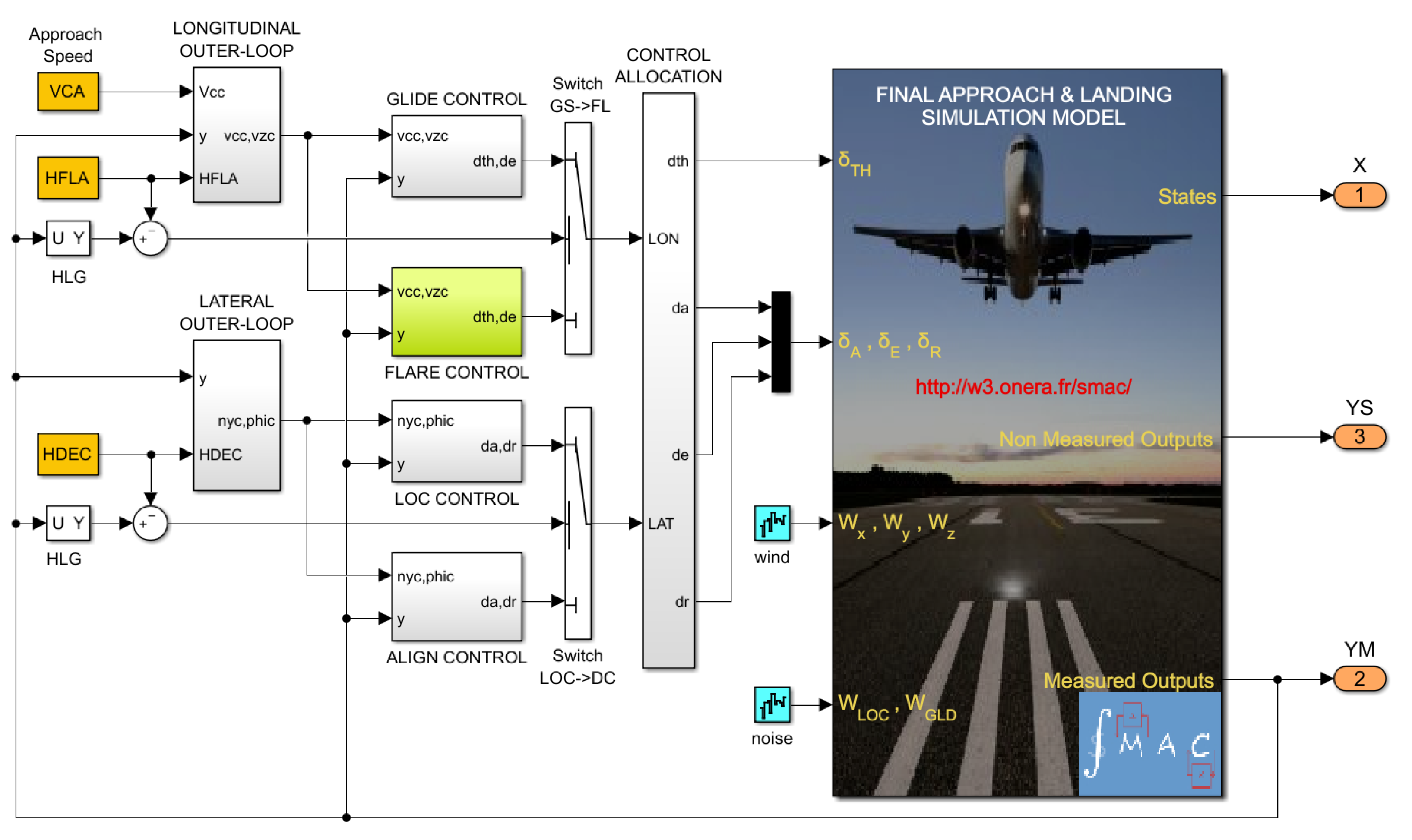
The structured flare control law resulting from the above optimization process was implemented in a nonlinear closed-loop simulation diagram, as shown in Figure 5. The flare system, highlighted in green, is activated as soon as the height of the landing gear is lower than a prescribed value , which has been classically set here to ft. To illustrate the benefits of using the longitudinal speed variations during the flare phase, two different controllers are compared with deterministic windsteps first and then with turbulences and ILS noises. Next, specific simulations also illustrate the robustness of the proposed controller by comparing the results of different values of the mass and the center-of-gravity location.
4.1. On the Interest of Using the Airspeed During Flare: Comparison of Laws I & II
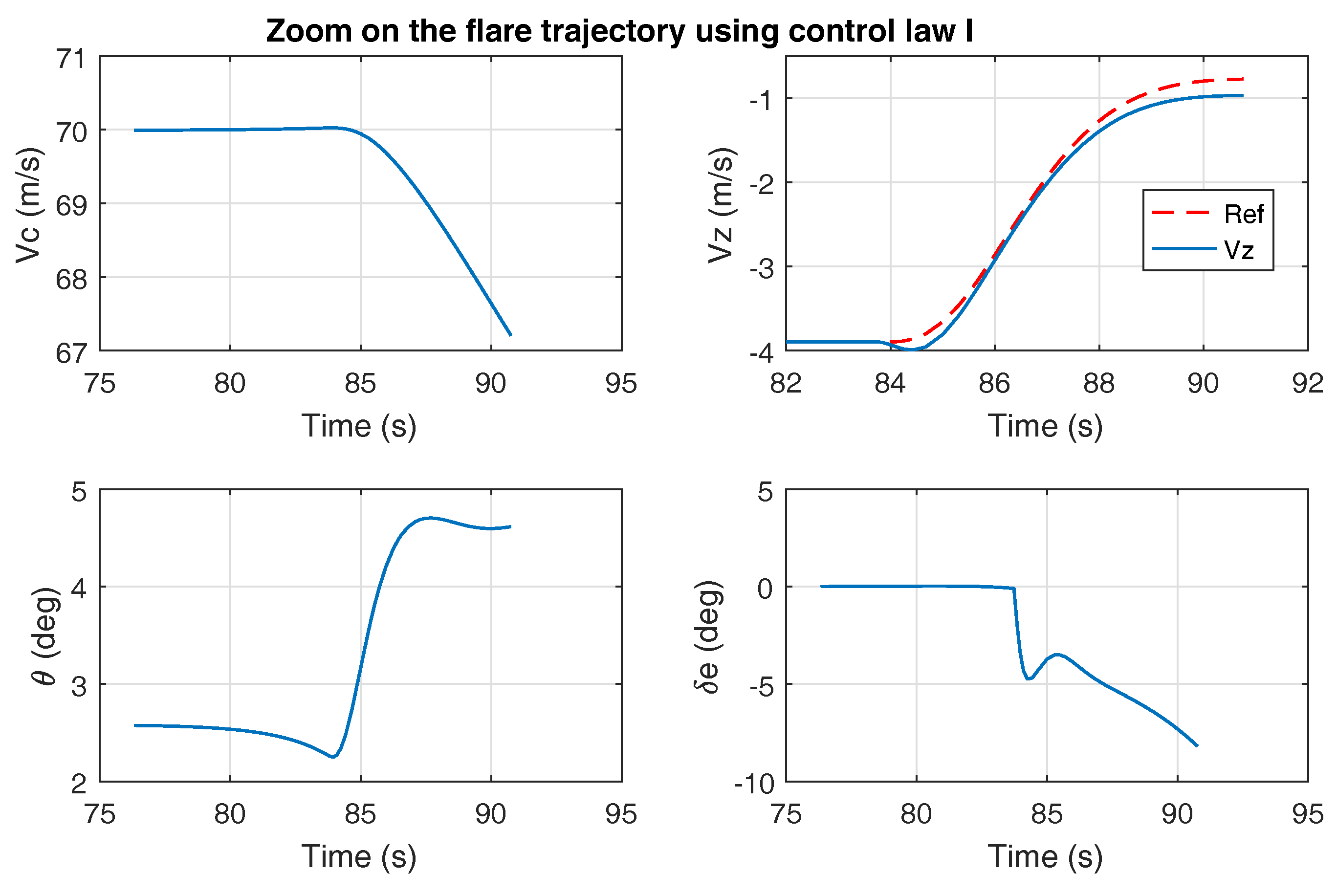
In a nominal mass and centering configuration ( and ), the last s of simulation before touchdown (thus focusing on the flare trajectory) are displayed in Figure 6 and Figure 7.
A comparison of the upper-right plots clearly shows that the second controller (using airspeed) outperforms the first one. The second controller is thus used for the remainder of the simulations. In this last case indeed, the vertical speed profile is very close to the reference represented by the dash-dotted red line.
4.2. Wind & Turbulence Effects
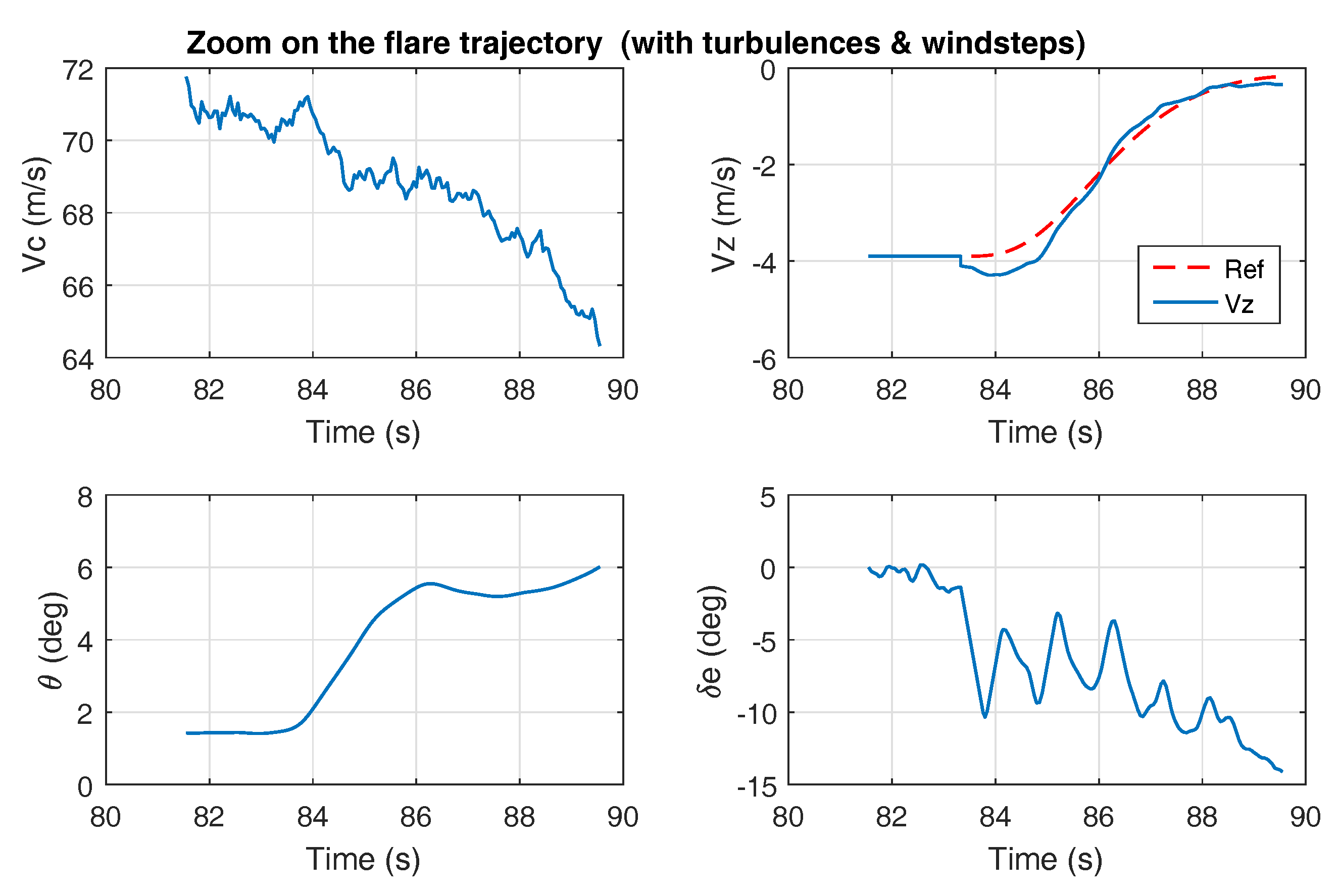
Deterministic windsteps and turbulence effects are then analyzed in the following simulations displayed in Figure 8, Figure 9 and Figure 10. In the first two figures, the global trajectory (final approach and flare) is visualized.
In the first case, a windstep is applied at s (see the upper-right subplot of Figure 8). In the second case (Figure 9), strong turbulence conditions are added. In both situations, the proposed guidance and control system behaves well. The impact point is slightly m after the hreshold meets the requirements.
Moreover, as is displayed in Figure 10, a zoom on the flare trajectory reveals that the vertical speed remains close to the reference trajectory (upper-right subplot). It is also noted that, during the flare maneuver, the pitch angle is barely decreasing. This property is of high interest to make the autoland system compatible with standard pilots habits.
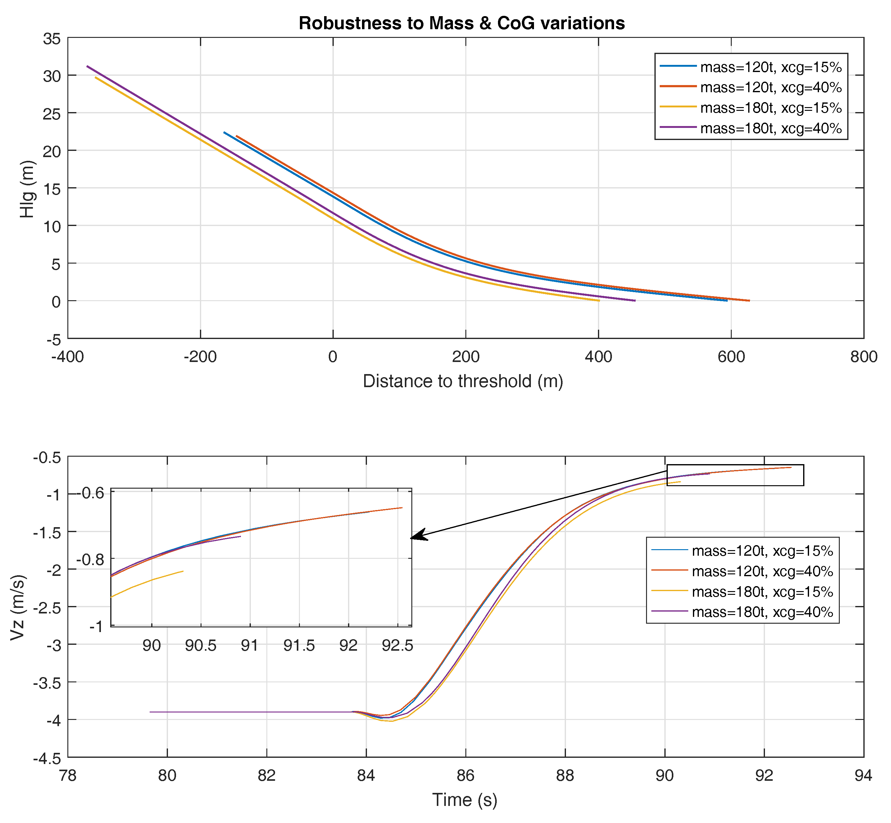
4.3. Illustration of Robustness
To conclude this section, the robustness of the proposed autoland control system is now evaluated through various simulations corresponding to the four extreme configurations of the mass (varying between t and t) and the center-of-gravity location (). The results (showing the two most critical variables in the longitudinal axis, namely, the height of the landing gear and the vertical speed) are presented in Figure 11. A reasonable dispersion of the impact point (lying in the interval ) is observed. It can also be pointed out that the vertical speed is well tracked whatever the flight condition.
5. Conclusions
A new multi-model -based design approach has been proposed and evaluated in this paper to improve and shorten the tuning process of flare control systems. Exploiting new capabilities of optimization tools, the proposed methodology allows to design a fast and accurate vertical controller despite measured (longitudinal speed variations) and external (wind) perturbations. Thanks to this new controller, the flare outer-loop design becomes much easier and the safety of the whole maneuver is improved. Moreover, thanks to a flexible framework enabled by a multi-model strategy, robustness characteristics against parametric uncertainties and modeling errors are easily taken into account. This is achieved here to enforce robustness against inaccurate modeling of the ground effects and significant variations of the mass and the center-of-gravity location.
Author Contributions
Jean-Marc Biannic and Clément Roos jointly developed the nonlinear aircraft model and the flare control design methodology; the controller gains tuning and nonlinear simulations were initially performed by Jean-Marc Biannic and then updated by Clément Roos; Jean-Marc Biannic and Clément Roos jointly wrote the paper and its revised version.
Conflicts of Interest
The authors declare no conflict of interest.
Appendix A. The Aircraft Model
Appendix A.1. General Equations
Following a standard approach, the aircraft model is obtained from the dynamics and kinematics equations. Let us denote and , the angular and translation velocity vectors both expressed in a body axis frame with respect to the center of gravity of the aircraft. One obtains
and
where m denotes the mass of the aircraft and is the inertia matrix. The two vectors and stand for the moments and forces vectors to be detailed next. However, the differential equations first should be finalized first. To this end, let us introduce and . The first vector contains the Euler angles (bank, pitch, and heading, respectively). The second one contains the position of the center of gravity G of the aircraft. They are both expressed in an earth-linked vertical frame. The x-axis is oriented forward, the y-axis is oriented rightward, and the z axis is oriented downward. The kinematics and navigation equations yield, respectively,
and
where the transformation and rotation matrices and are defined in Equations (A5) and (A6) below, respectively:
The 12th order aircraft model can thus be summarized as follows:
Appendix A.2. Forces and Moments
The forces applied to the aircraft can be decomposed into three terms (engines thrust, gravity, and aerodynamic forces):
To comply with Equation (A1), these must also be expressed in the body-axis frame. Assuming that the thrust is aligned with the longitudinal axis, one obtains
The gravity forces in the body-axis frame are given by
Finally, the aerodynamic forces, initially expressed in a stability-axis frame, are obtained as
where , , and S denote the angle-of-attack, the dynamic pressure (see Equation (A15)), and the reference surface, respectively. The drag (), lateral (), and lift () coefficients are detailed in Section A.4.
The moment M about the center of gravity G of the aircraft results from the engines thrust and aerodynamic actions:
Assuming that both engines deliver the same thrust, its location can be reduced to a single point E whose coordinate along the y-axis is zero. The moment resulting from the thrust is
Note that the engines are located below the center of gravity, such that and one observes a pitching moment. The aerodynamic moment exhibits two terms:
The first one contains the main contribution and is directly proportional to the moment coefficients , , and (about roll, pitch, and yaw axes, respectively) and to the aerodynamic mean chord L. The second term is linked to the fact that the point of application A of the aerodynamic forces possibly differs from the center of gravity G (which may change during flight with fuel consumption).
Appendix A.3. Wind and Atmosphere Effects
Aerodynamic moments and forces strongly depend on the airspeed , but also on the air density , via the dynamic pressure:
The airspeed is clearly affected by wind. The latter denoted is generally expressed in an earth-linked vertical frame. The airspeed vector in body-axis coordinates is thus obtained as
Aerodynamic coefficients also depend on the aerodynamic angle-of-attack and sideslip angle which are respectively obtained as
Let us now detail the expression of , which depends on altitude and temperature. During the landing phase, from approximately ft above the runway until touchdown, the altitude and temperature variations are negligible. The air density can then be viewed as a fixed parameter depending on the runway altitude and temperature. Let us denote (expressed in m), the runway altitude, and (expressed in K), the temperature at sea-level. Since the maximum value for is about 3000 m, the temperature at runway level is well approximated by
and
At low altitudes and speeds, the calibrated airspeed describing the dynamic pressure acting on aircraft surfaces regardless of air density is quite close to the equivalent airspeed and is then obtained from the true airspeed as follows:
where stands for the air density at sea-level for a nominal temperature K. Finally, the Mach number, which impacts the engine efficiency, is defined as the ratio between airspeed and sound-speed at the runway level:
with
Appendix A.4. Aerodynamic Coefficients
Let us define the ailerons, elevators, and rudders deflections , , and . The lift, lateral and drag coefficients are, respectively, given by
Note that the last term in the lift coefficient describes the ground effect. The lift increases as the aircraft becomes closer to the ground. The variable in this term denotes the height of the main landing gear above runway. Similarly, the moment coefficients about x, y, and z axes are given by
Here again, the last term on the pitching moment in Equation (A27) corresponds to the ground effect (nose down).
Appendix A.5. Engines and Actuators
During the final approach and landing phases, the aircraft is controlled by means of
- twin engines that both provide the same thrust in the fuselage direction (x-axis),
- a pair of ailerons whose asymmetric deflection generates moments about the x-axis (roll),
- an elevator whose deflection controls the y-axis (pitch), and
- a rudder whose deflection controls the z-axis (yaw).
The dynamics of the engines and actuators are approximated by magnitude and rate limited first-order filters in the following generic format:
where is the commanded value of , and is the time constant. All numerical values are summarized in Table A1.

Table A1.
Engines & actuators characteristics.
| Control Input () | Time Constant () | Lower Bound () | Upper Bound () | Rate Limit () |
|---|---|---|---|---|
| Engines () | s | |||
| Ailerons () | s | deg | deg | deg/s |
| Elevators () | s | deg | deg | deg/s |
| Rudder () | s | deg | deg | deg/s |
Remark A1.
The effective thrust at a given altitude, which appears in Equation (A9), is approximated by an affine function of the exhaust pressure ratio (EPR also denoted by the symbol ):
whose coefficients depend on the temperature ratio . In this application, since the temperature ratio during landing exhibits small variations, mean constant values can be considered. The following expression will then be used:
where .
Remark A2.
Along the longitudinal axis, the aircraft is trimmed by the horizontal stabilizers whose dynamics are much slower than those of the elevators. It is assumed that the stabilizers are not used during the final approach, so they are not represented here.
Appendix A.6. SIMULINK® Implementation
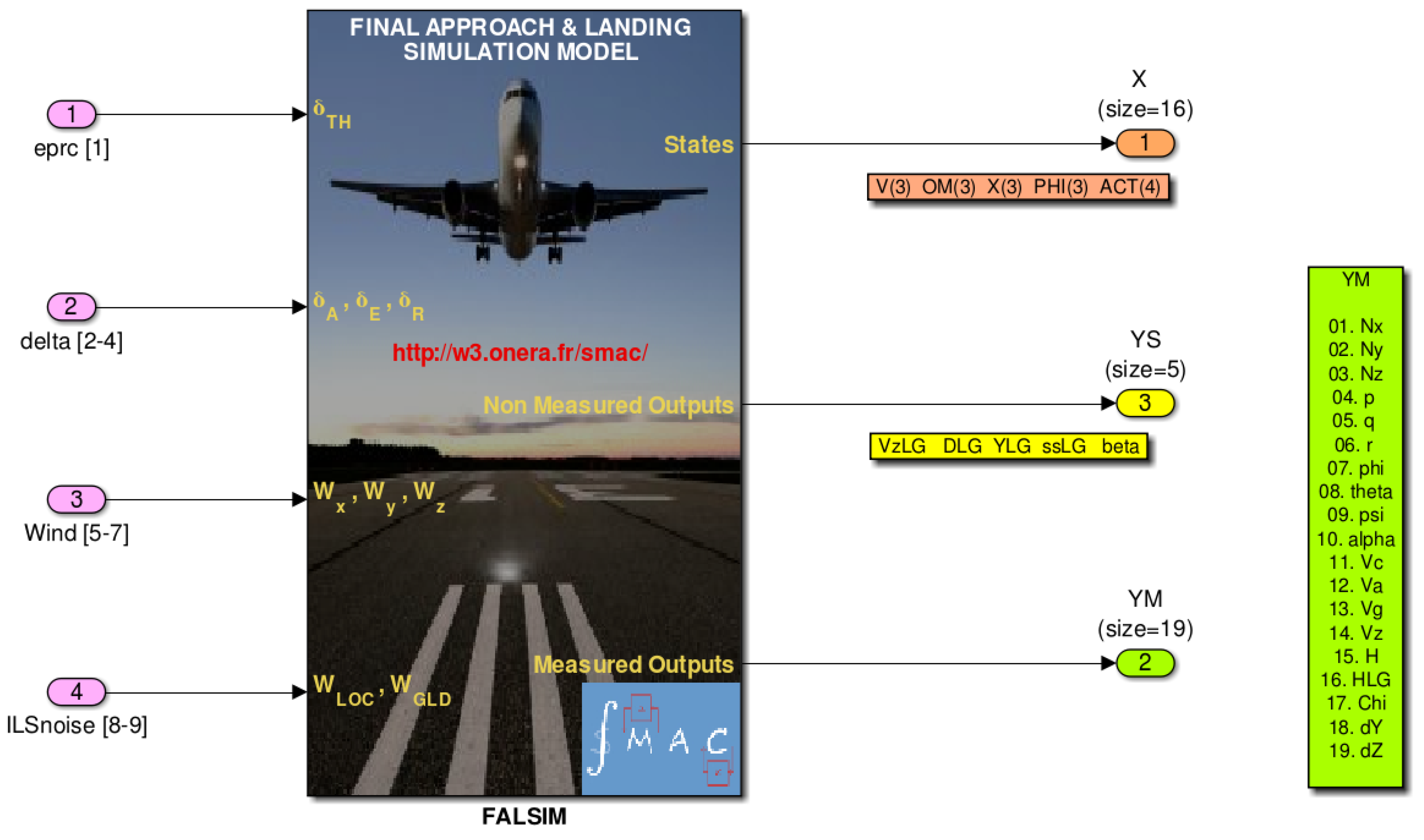
The above equations are implemented in an open-access diagram ACS.slx (Figure A1) whose main block “FALSIM” (for Final Approach & Landing SImulation Model) exhibits 9 inputs (4 control inputs, 3 wind inputs, and 2 ILS noises inputs) and 40 outputs. The first 16 ones correspond to the state vector (including actuators dynamics). The next 5 correspond to simulation oriented signals. These are not available for feedback. Finally, the last 19 outputs are measured signals. Note that the last two ( and ) correspond, respectively, to the lateral and vertical deviations from the nominal trajectory. These are delivered by the ILS device.
For control and simulation purposes, the model is delivered with a routine ACStrim.m to enable fast trimming and linearization of the nonlinear model. Various linear representations can thus be easily obtained according to the selected approach speed, initial slope, runway altitude, temperature, mass, and center-of-gravity location.
Figure A1.
A general view of the aircraft simulation model.

This model and the associated tools can be downloaded from the benchmark section of the SMAC project (http://w3.onera.fr/smac), where a technical note co-signed by Onera and Airbus is also available [17]. The latter includes a brief description of the aircraft model but is mainly focused on autoland design guidelines and requirements. It was written to offer control researchers a realistic and challenging autoland design problem and to promote competition in this field. It is quite interesting to note that a number of high-quality contributions have already been reported [18,19].
References
- Airbus. A Statistical Analysis of Commercial Aviation Accidents 1958–2016; Technical Report; Airbus: Toulouse, France, 2017. [Google Scholar]
- Kaminer, I.; Khargonekar, P. Design of the Flare Control Law for Longitudinal Autopilot Using H∞ Synthesis. In Proceedings of the 29th IEEE Conference on Decision and Control, Honolulu, HI, USA, 5–7 December 1990; pp. 2981–2986. [Google Scholar]
- Biannic, J.M.; Apkarian, P. A New Approach to Fixed-order H∞ Synthesis: Application to Autoland Design. In Proceedings of the AIAA Guidance, Navigation, and Control Conference, Monterey, CA, USA, 6–9 August 2001. [Google Scholar]
- Looye, G.; Joos, H. Design of Autoland Controller Functions with Multiobjective Optimization. J. Guid. Control Dyn. 2006, 29, 475–484. [Google Scholar] [CrossRef]
- Sadat-Hoseini, H.; Fazelzadeh, A.; Rasti, A.; Marzocca, P. Final Approach and Flare Control of a Flexible Aircraft in Crosswind Landings. J. Guid. Control Dyn. 2013, 36, 946–957. [Google Scholar] [CrossRef]
- Isidori, A.; Marconi, L.; Serrani, A. Robust Nonlinear Motion Control of a Helicopter. IEEE Trans. Autom. Control 2003, 48, 413–426. [Google Scholar] [CrossRef]
- Peng, K.; Cai, G.; Chen, B.; Dong, M.; Lum, K.; Lee, T. Design and implementation of an autonomous flight control law for a UAV helicopter. Automatica 2009, 45, 2333–2338. [Google Scholar] [CrossRef]
- Magni, J.F. Multimodel Eigenstructure Assignment in Flight-Control Design. Aerosp. Sci. Technol. 1999, 3, 141–151. [Google Scholar] [CrossRef]
- Dorobantu, A.; Murch, A.; Balas, G. Robust Control Design for the NASA AirSTAR Flight Test Vehicle. In Proceedings of the 50th AIAA Aerospace Sciences Meeting, Nashville, TN, USA, 9–12 January 2012. [Google Scholar]
- Apkarian, P.; Noll, D. Nonsmooth H∞ Synthesis. IEEE Trans. Autom. Control 2006, 51, 71–86. [Google Scholar] [CrossRef]
- Burke, J.; Henrion, D.; Lewis, A.; Overton, M. Stabilization via Nonsmooth, Nonconvex Optimization. IEEE Trans. Autom. Control 2006, 51, 1760–1769. [Google Scholar] [CrossRef]
- Apkarian, P.; Gahinet, P.; Buhr, P. Multi-Model, Multi-Objective Tuning of Fixed-Structure Controllers. In Proceedings of the European Control Conference, Strasbourg, France, 24–27 June 2014; pp. 856–861. [Google Scholar]
- Biannic, J.M.; Roos, C. Flare Control Law Design via Multi-Channel H∞ Synthesis: Illustration on a Freely Available Nonlinear Aircraft Benchmark. In Proceedings of the American Control Conference, Chicago, IL, USA, 17–19 June 2015; pp. 1303–1308. [Google Scholar]
- Zhou, K.; Doyle, J. Essential of Robust Control; Prentice-Hall: Upper Saddle River, NJ, USA, 1998. [Google Scholar]
- Biannic, J.M.; Roos, C.; Lesprier, J. Nonlinear Structured H∞ Controllers for Parameter-Dependent Uncertain Systems with Application to Aircraft Landing. AerospaceLab J. 2017, 13. [Google Scholar] [CrossRef]
- The Mathworks Inc. Robust Control Toolbox. Available online: https://mathworks.com/products/robust.html (accessed on 8 February 2016).
- Biannic, J.M.; Boada-Bauxell, J. A Civilian Aircraft Landing Challenge. Online Available from the Aerospace Benchmark Section of the SMAC Toolbox. Available online: http://w3.onera.fr/smac/ (accessed on 8 February 2016).
- Navarro-Tapia, D.; Simplicio, P.; Iannelli, A.; Marcos, A. Flare Control Design Using Structured H∞ Synthesis: A Civilian Aircraft Landing Challenge. In Proceedings of the 20th IFAC World Congress, Toulouse, France, 9–14 July 2017; pp. 4032–4037. [Google Scholar]
- Theis, J.; Ossmann, D.; Pfifer, H. Robust Autopilot Design for Crosswind Landing. In Proceedings of the 20th IFAC World Congress, Toulouse, France, 9–14 July 2017. [Google Scholar]
Figure 1.
Basic segments of the approach and landing maneuver in a vertical plane.

Figure 2.
Autoland architecture.

Figure 3.
Flare control system.
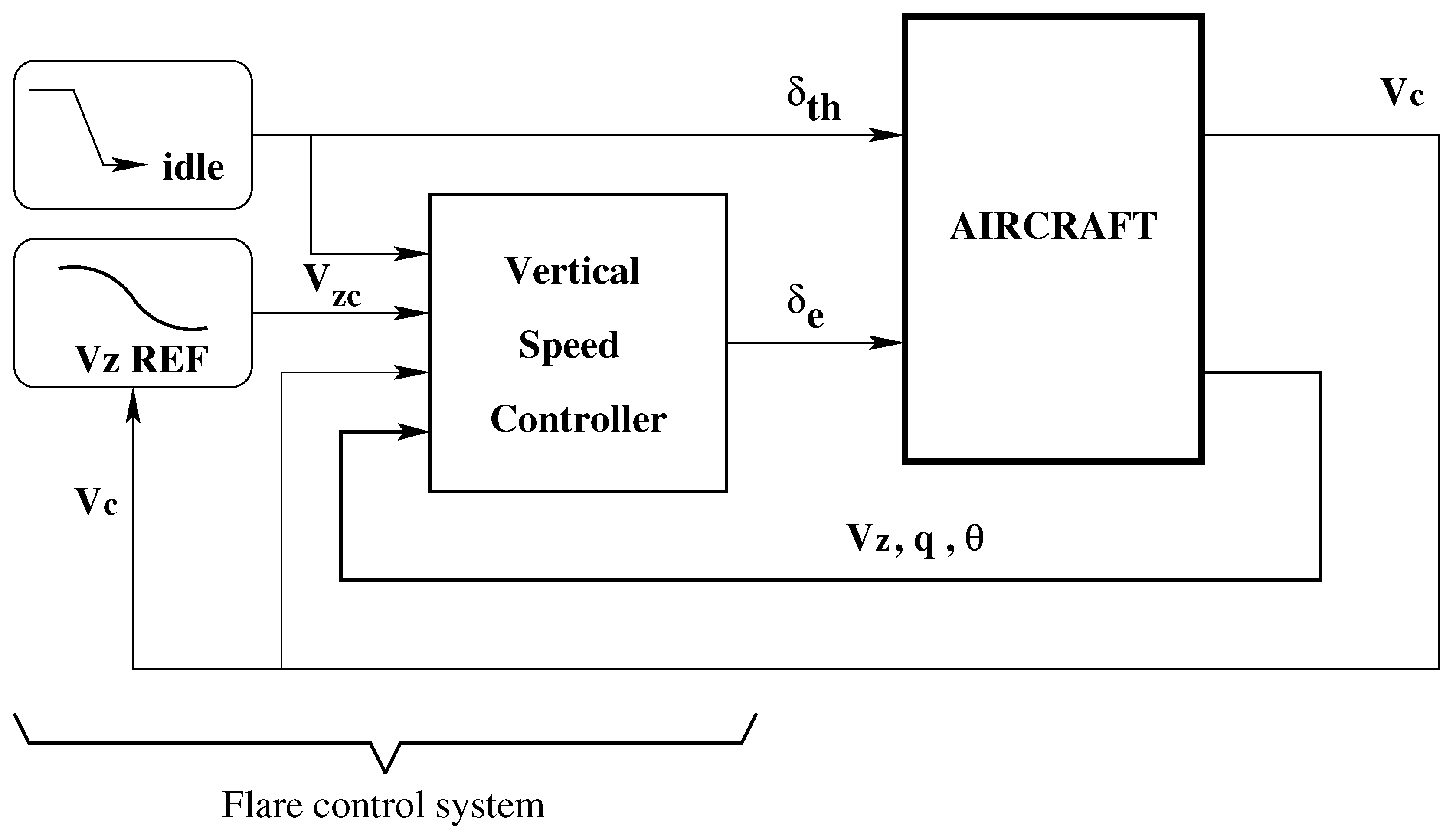
Figure 4.
Design model.
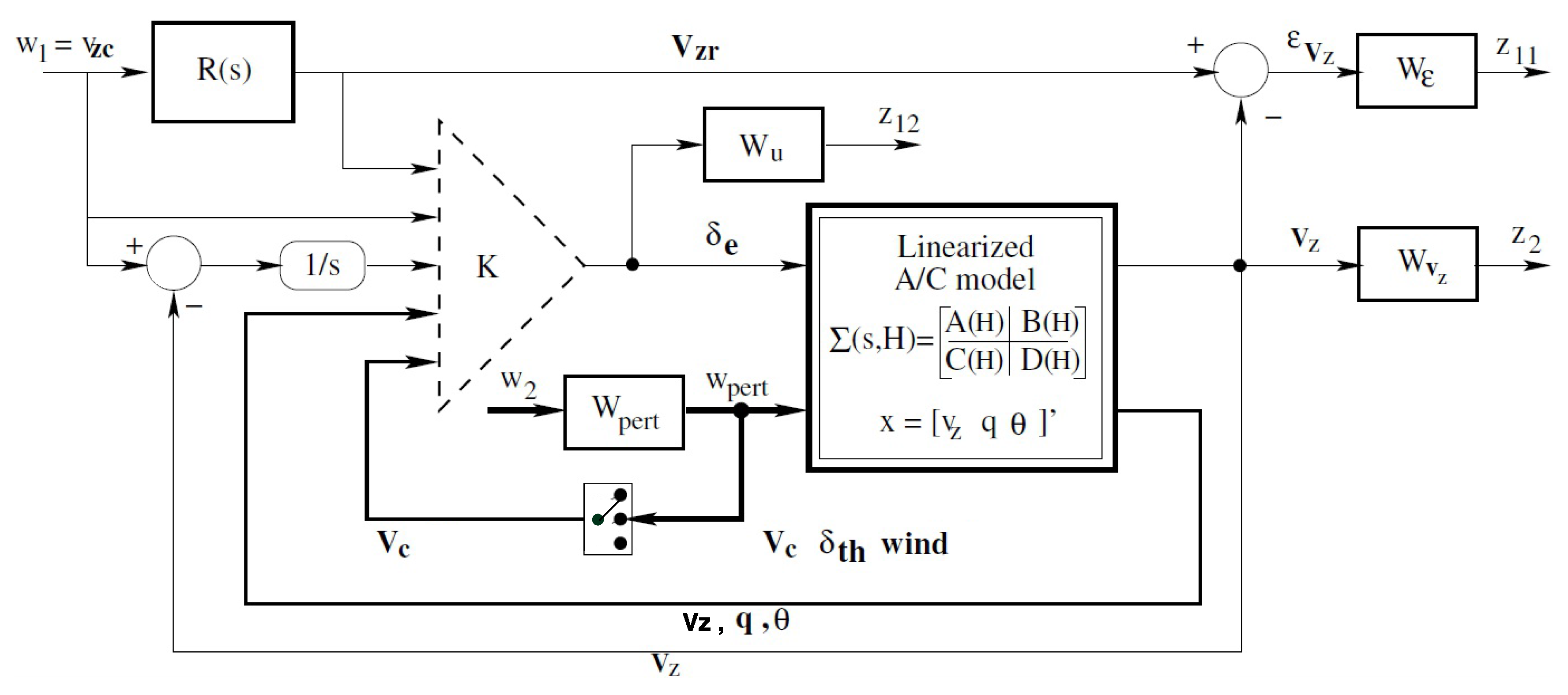
Figure 5.
Nonlinear closed-loop simulation model.

Figure 6.
Flare trajectory with Control Law I (without speed feedback).

Figure 7.
Flare trajectory with Control Law II (with speed feedback).
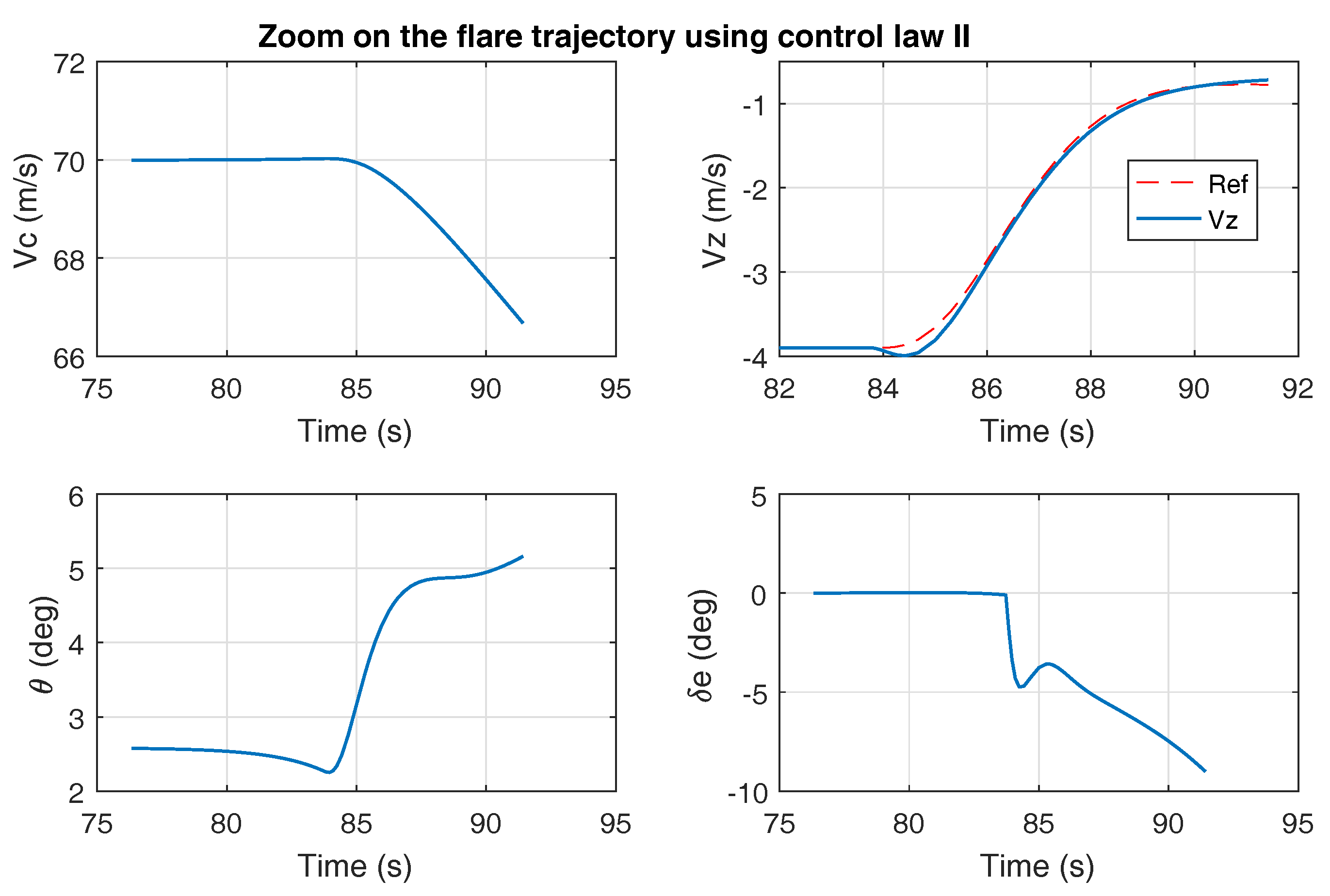
Figure 8.
Final approach and flare trajectory with deterministic windsteps.
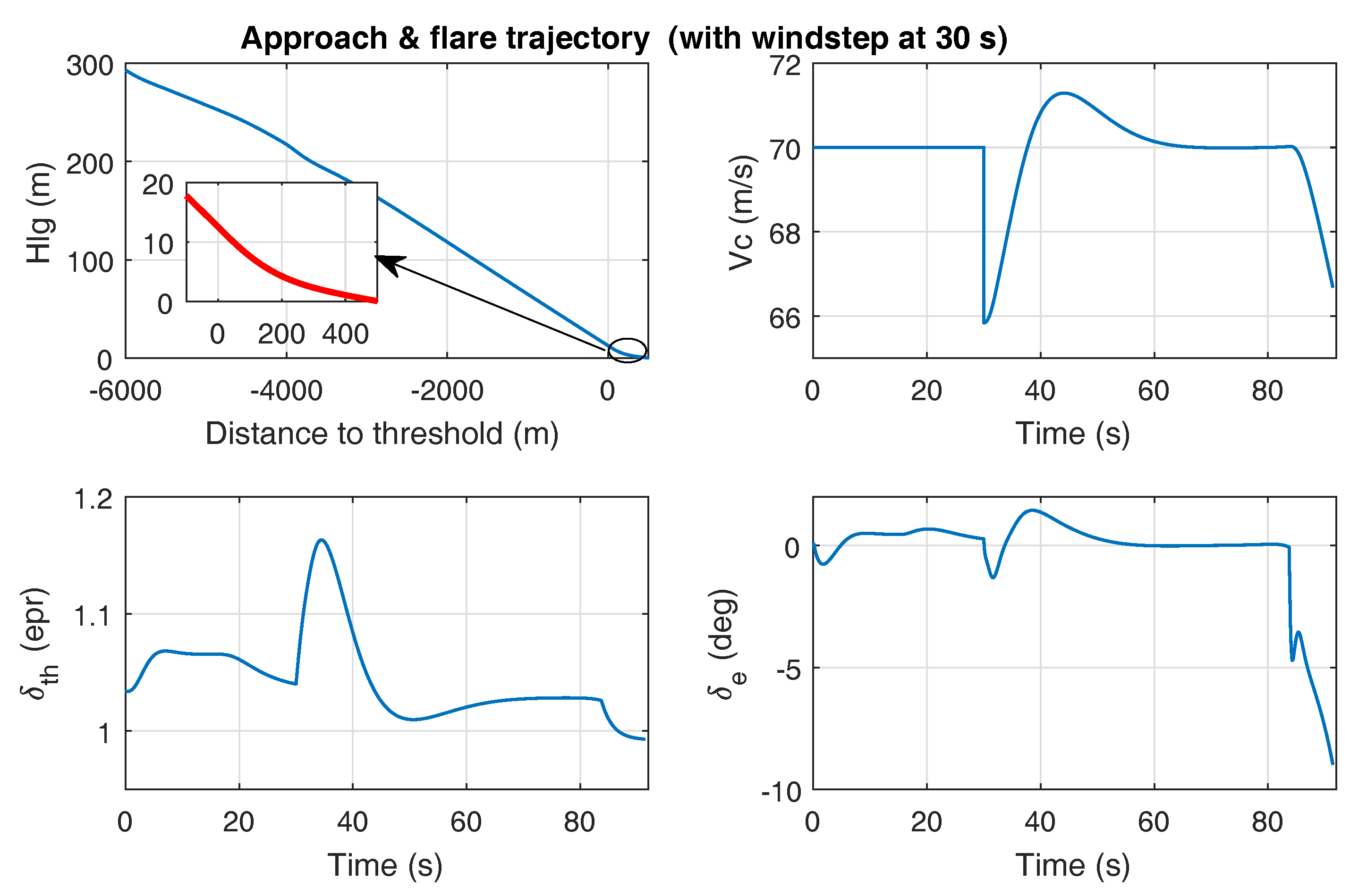
Figure 9.
Final approach and flare trajectory with deterministic windsteps and turbulences.
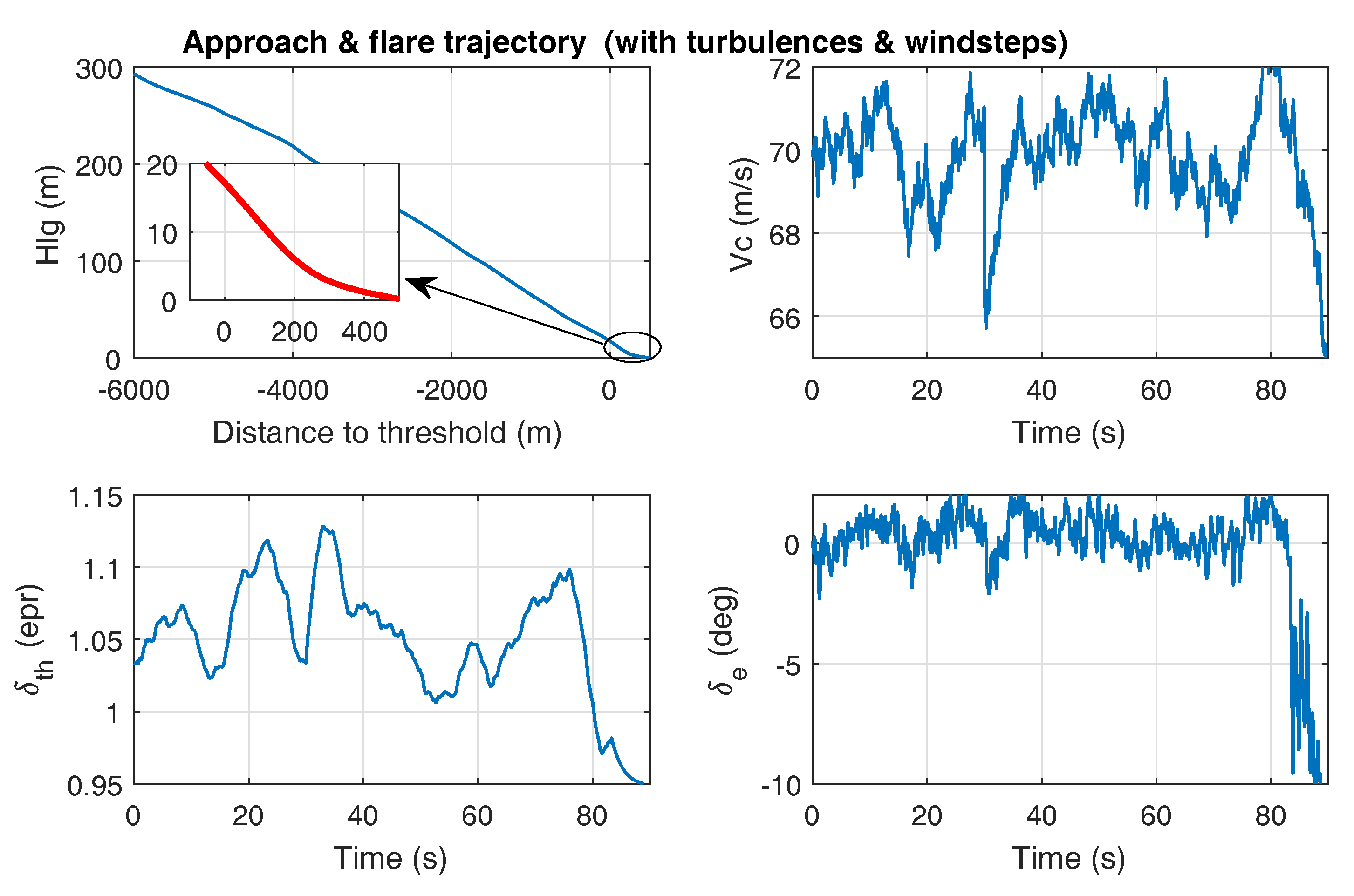
Figure 10.
Zoom on the flare trajectory with deterministic windsteps and turbulences.

Figure 11.
Robustness to mass and center-of-gravity variations.
© 2018 by the authors. Licensee MDPI, Basel, Switzerland. This article is an open access article distributed under the terms and conditions of the Creative Commons Attribution (CC BY) license (http://creativecommons.org/licenses/by/4.0/).
Share and Cite
MDPI and ACS Style
Biannic, J.-M.; Roos, C. Robust Autoland Design by Multi-Model ℋ∞ Synthesis with a Focus on the Flare Phase. Aerospace 2018, 5, 18. https://doi.org/10.3390/aerospace5010018
AMA Style
Biannic J-M, Roos C. Robust Autoland Design by Multi-Model ℋ∞ Synthesis with a Focus on the Flare Phase. Aerospace. 2018; 5(1):18. https://doi.org/10.3390/aerospace5010018
Chicago/Turabian StyleBiannic, Jean-Marc, and Clément Roos. 2018. "Robust Autoland Design by Multi-Model ℋ∞ Synthesis with a Focus on the Flare Phase" Aerospace 5, no. 1: 18. https://doi.org/10.3390/aerospace5010018
Note that from the first issue of 2016, this journal uses article numbers instead of page numbers. See further details here.