Design of a Facility for Studying Shock-Cell Noise on Single and Coaxial Jets


1
Aeronautics and Aerospace Department, von Karman Institute for Fluid Dynamics, Chaussée de Waterloo 72, 1640 Rhode-Saint-Genèse, Belgium
2
Faculty of Aerospace Engineering, Delft University of Technology, Building 62, Kluyverweg 1, 2629 HS Delft, The Netherlands
*
Author to whom correspondence should be addressed.
Aerospace 2018, 5(1), 25; https://doi.org/10.3390/aerospace5010025
Submission received: 12 January 2018
/
Revised: 24 February 2018
/
Accepted: 25 February 2018
/
Published: 1 March 2018
(This article belongs to the Special Issue Under-Expanded Jets)
Abstract
:Shock-cell noise occurs in aero-engines when the nozzle exhaust is supersonic and shock-cells are present in the jet. In commercial turbofan engines, at cruise, the secondary flow is often supersonic underexpanded, with the formation of annular shock-cells in the jet and consequent onset of shock-cell noise. This paper aims at describing the design process of the new facility FAST (Free jet AeroacouSTic laboratory) at the von Karman Institute, aimed at the investigation of the shock-cell noise phenomenon on a dual stream jet. The rig consists of a coaxial open jet, with supersonic capability for both the primary and secondary flow. A coaxial silencer was designed to suppress the spurious noise coming from the feeding lines. Computational fluid dynamics (CFD) simulations of the coaxial jet and acoustic simulations of the silencer have been carried out to support the design choices. Finally, the rig has been validated by performing experimental measurements on a supersonic single stream jet and comparing the results with the literature. Fine-scale PIV (Particle Image Velocimetry) coupled with a microphone array in the far field have been used in this scope. Preliminary results of the dual stream jet are also shown.
1. Introduction
This work is aimed at describing the design and the commissioning of a new supersonic coaxial jet rig to investigate experimentally the shock-cell noise on dual stream jets. This kind of noise is nowadays an important component of the total noise emitted by aeronautic engines, particularly affecting cabin noise in cruise conditions. The target maximum achievable Mach number at the outlet of the primary (core) and secondary (fan) nozzle is equal to , with a baseline operating point being and . The literature on the shock-associated noise is rich in studies in terms of experiments [1,2,3,4], modeling [5,6,7,8] and, more recently, advanced CFD and CAA studies [9,10,11,12]. Most of this research, however, is focused on single stream supersonic jets. The objective of this facility is to progress further in complexity, making use of a coaxial jet, with subsonic primary flow and supersonic secondary flow, in order to increase the similitude with turbofan engines. It should be stressed at this stage that the primary flow is unheated, leading to a reversed velocity profile to yield the desired Mach numbers in each stream. Nevertheless, it is still a valuable benchmark for physical understanding and validation of theoretical or numerical models because of the annular shock-cells’ pattern confined between two shear layers.
2. Facility Design Process
A first assessment of the requirements has been performed based on the case already investigated experimentally by Viswanathan et al. [13] and numerically by Miller and Morris [14]. The initial flow parameters for the coaxial jet are and for the primary and secondary flow, respectively. As a constraint, an indicative total mass flow of kg/s has been selected.
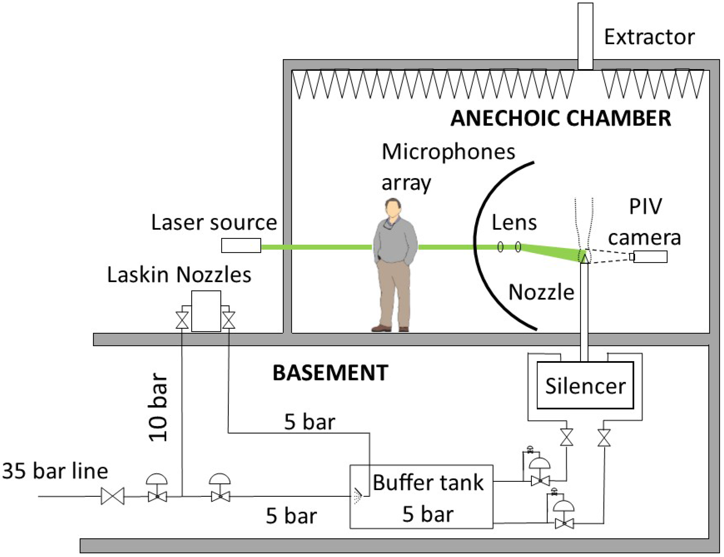
The chosen solution is a trade-off between a continuous and a blow-down facility. The facility is supplied by the VKI pressure distribution system at 35 bar, for a test duration exceeding 20 min. A single buffer tank is used to damp pressure oscillations from the pipeline and to introduce the seeding particles for the PIV measurements, ensuring a uniform mixing. In order to control the air supply, several pressure regulators have been implemented.
The flow enters the circuit at 35 bar (bottom left of Figure 1). An electrical ball valve with a safety return battery is used as the main ON/OFF shutter. A manual ball valve is placed upstream as backup. Successively, the pressure is decreased from 35 to 10 bar by means of two identical pressure regulators. This solution was necessary to fulfill the required volumetric flow. Downstream the twin regulators, part of the flow is diverted to the seeding generator, while the rest of the flow enters the buffer tank. A pilot-controlled pressure regulator lowers the pressure from 10 to 5 bar.
The seeded flow merges with the main stream flow into the buffer tank, which has a volume of 500 L, guaranteeing a residence time of the flow of the order of s. In this way, the seeding has the time to mix uniformly with the main stream flow. The tank is equipped with a safety rupture disk, which will break in case the pressure exceeds the tank limit of 11 bar.
From the buffer tank, two independent pressure lines are derived, each equipped with the same set of regulators, for commonality. Only on the primary flow line, a conditioning orifice flow meter is installed in order to directly measure the mass flow rate of the primary stream. It has been assessed by means of CFD simulations (described in Section 5). that it is impossible to calculate the primary mass flow rate by simply using the isentropic relations, because of shock-waves present in the secondary flow.
The two streams successively enter a coaxial silencer (described in Section 4), with low pressure losses, and compatible with the passage of oil particles. The purposes of this silencer are two-fold: firstly, to reduce the amount of noise coming from the air supply system, which would otherwise pollute the acoustic measurements; secondly, to prevent spurious, uncontrolled acoustic excitations of the jet. In that respect, the silencer should provide a good upstream anechoic termination for the nozzles, by preventing duct standing modes (not evaluated in this work). The flow enters into the coaxial silencer trough 20 radially-distributed inlets, 10 per each of the two circuits. Two conical flow distributors are used at this scope, each of them mounting 10 flexible pipes of the same length.
Downstream the silencer, the two flows are guided by vertical coaxial ducts into the anechoic chamber. Each duct is equipped with honeycombs and three fine turbulence screens. The ducts’ internal diameters are mm and mm for the primary and secondary flows, respectively. For the designed test campaigns, the Mach number in the ducts is lower than M = 0.05, and thus, the static pressure, measured upstream the nozzles, is considered to be the total pressure.
3. Facility Components
In this section, two key components of the facility are described: the coaxial nozzles and the silencer. For a complete description of more standard components such as valves, pressure regulators and pressure sensors, the reader is referred to Guariglia [15].
Coaxial Nozzles
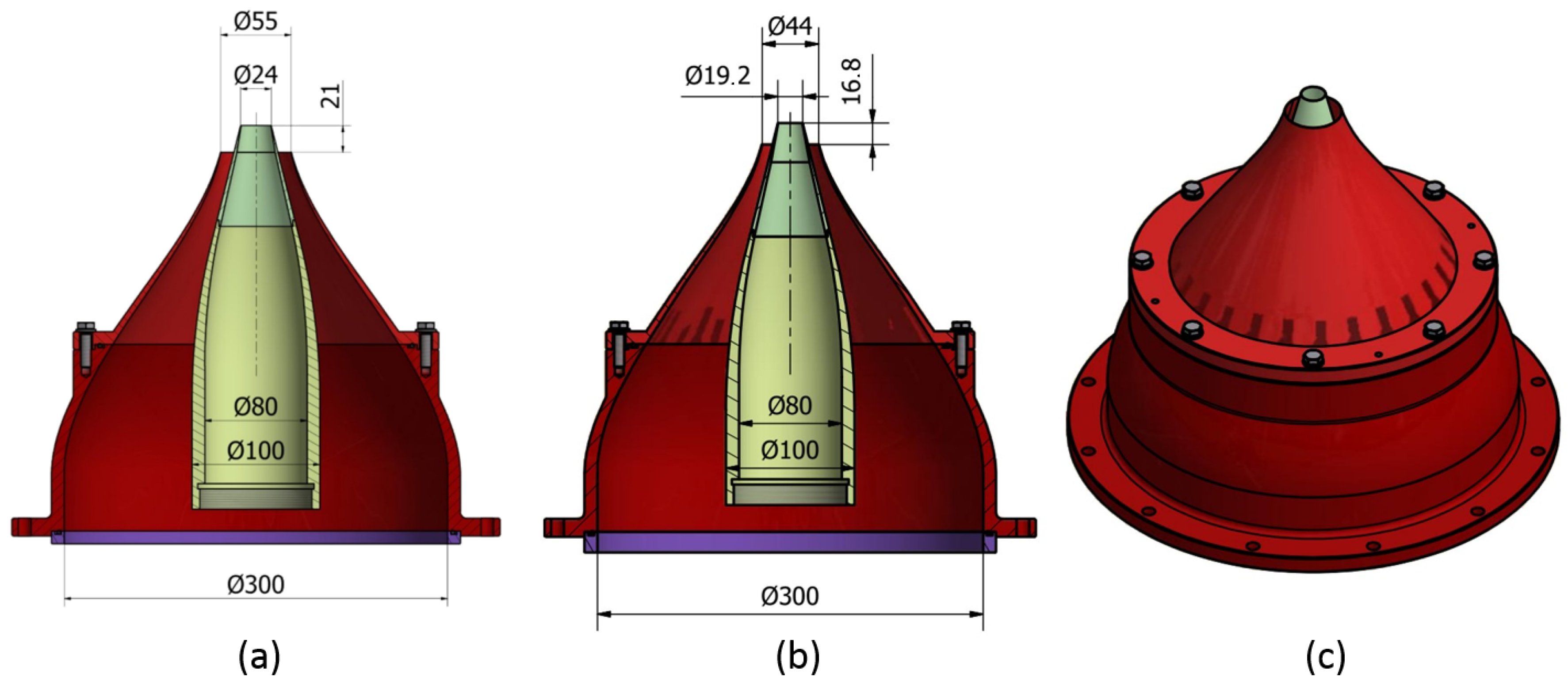
Two sets of coaxial nozzles have been designed and manufactured, following a layout proposed by Airbus, partner of the project. The geometry is representative of the next generation aeronautic engines with a very high by-pass ratio. For the first set, the nozzle diameters are mm and mm for the primary and secondary jets, respectively. The lip thickness is mm for both nozzles. The primary outlet plane is 21 mm downstream of the plane of the secondary outlet, and so, . The primary jet area contraction ratio is , and the secondary jet contraction ratio is . The primary nozzle has a simple conical shape, with the semi-aperture angle °. The secondary nozzle profile follows a third order polynomial function, modified ad hoc in the last part to have the sonic throat at the exit plane. The exit semi-aperture angle for the secondary nozzle is °. A section of the nozzles is depicted in Figure 4a. This nozzle set has been simulated with CFD and tested for the initial commissioning of the facility.
The second set of nozzles is just a scaled version of the previous ones. The goal is to assess the experiment repeatability and the jet noise spectra similarity for the single stream jet. The scaling factor is 0.8; thus, mm, mm, and the primary outlet plane is 16.8 mm downstream of the plane of the secondary outlet (Figure 4b).
Both nozzle sets were realized in stainless steel and painted with matte black paint to avoid reflections in PIV experiments. A metal ring spacer, placed under the secondary nozzle, can be modified in order to adjust the protrusion length of the primary nozzle.
4. Silencer
The design concept is based on having two U-turn annular sections, in order to maximize the area of the damping material exposed to the incident acoustic field, while minimizing the flow velocity and associated pressure losses (Figure 3c). The colored zones represent the clean passage areas, while the gray dashed zones are the acoustic absorbent material, which is a very fine stainless steel wool (Type #000). Due to space constraints, it has been decided to use a fixed thickness for all the layers, equal to mm. The clean passage areas have been sized in order to not exceed 10 m/s and reduce both pressure losses and extra noise production. The wool is held by four metal canisters. The relevant dimensions are summarized in Table 1.
Acoustic Performance
To assess the silencer acoustic performance before the manufacturing and to select the most appropriate absorbent material, the commercial solver COMSOL Multiphysics® 5.0 has been used. The Transmission Loss (TL) between the ten inlets and the nozzles outlet has been computed, including the effects of the acoustic absorbent material, the metal canisters holding it, a limited portion of the ducts (1 m, for computational efficiency) and the nozzles. The honeycomb and screens that are installed in the ducts are not modeled.
It is assumed that the medium is quiescent inside the silencer, so sound production and convection effects are neglected in the model. This hypothesis appears to be justified by the small flow Mach number inside (M) and considering also the important noise contribution due to the chocked valves upstream of the silencer. For the sake of brevity, the equations implemented in the model are not presented here, and the reader is referred to the COMSOL Multiphysics® 5.0 User Manual [16]. The physical quantities required to run the simulations are listed in Table 1.
Fifty frequencies in the range 100 Hz ≤ f ≤ 5000 Hz have been tested. Above this frequency interval, practical experience suggests that the noise is efficiently damped by the acoustic absorbent material.
The domain has been meshed with tetrahedral linear elements, with the maximum element length equal to 1/10th of the smallest computed wavelength. The inlet boundary condition is modeled as a harmonic pressure source of amplitude Pa, and it is applied to the surface of the 10 inlet pipes. This boundary condition is valid as long as the frequency is kept below the cutoff frequency for the second propagating mode in the tube [17], as happens in the case studied. At the outlet boundary, the model specifies a radiation condition for an outgoing plane wave, a valid assumption in the case studied. The walls are modeled as infinitely rigid boundaries.
The attenuation (in dB) of the acoustic power is defined by the following equation:
where and denote the incoming power at the inlet and the outgoing power at the outlet, respectively.
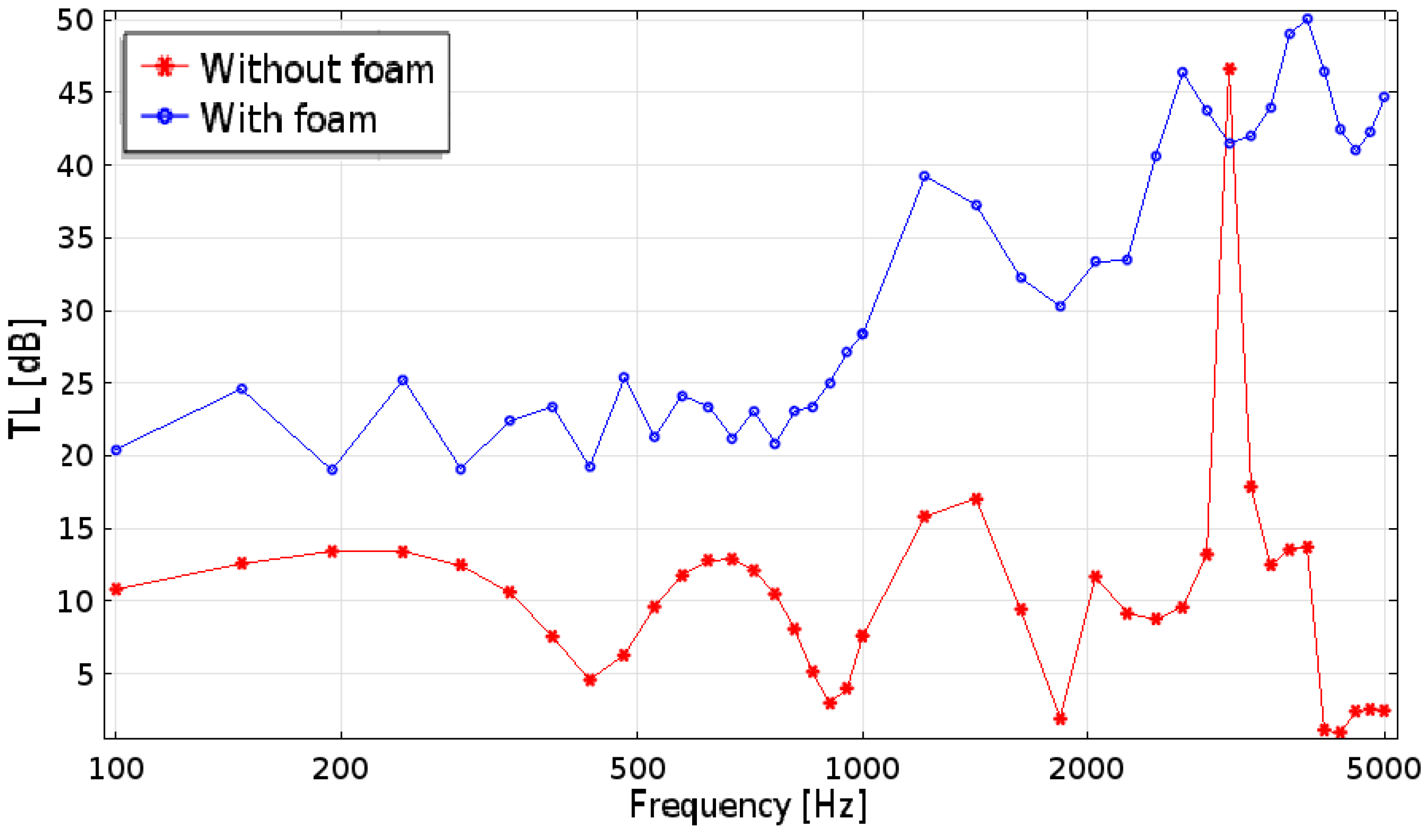
In Figure 5 and Figure 6, three characteristic acoustic fields, per circuit, are shown. The first field, at lower frequency, shows the presence of plane waves in all the domain; while increasing the frequency, more modes appear in the silencer and in the secondary duct. Such modes, however, naturally disappear when approaching the secondary nozzle, thus respecting the outlet boundary conditions. For both circuits, the TL has been computed with and without the absorbent material, and the results are shown in Figure 7 and Figure 8. Overall, the primary circuit appears very effective in damping the acoustic power. Below Hz, the geometry alone is very effective in damping the noise, while above Hz, the presence of the steel wool contributes significantly to the TL. On the other side, the secondary circuit is less effective, compared to the primary one, and the steel wool is important at all frequencies.
At the end of this acoustic assessment, the predicted levels of TL have been evaluated satisfactorily, in consideration of the frequencies expected during the tests, higher than 5000 Hz.
5. RANS Simulations of the Coaxial Jet
RANS simulations of the dual flow jet have been performed in order to verify that the flow at the nozzles exit matches the design conditions and to have a first insight into the flow field. The simulated geometry represents the Nozzle Set 1 (Figure 4a), and the results are considered extendible also to the scaled geometry. The computations have been carried out with COMSOL Multiphysics® 4.4 using linear triangular finite elements and 2D axisymmetric flow assumption. It should be stressed here that the goal of these simulations is only to validate the nozzle design and to provide useful insights into the flow fields for the development of the experimental setup.
5.1. Test Conditions
5.2. Fluid Dynamics Model
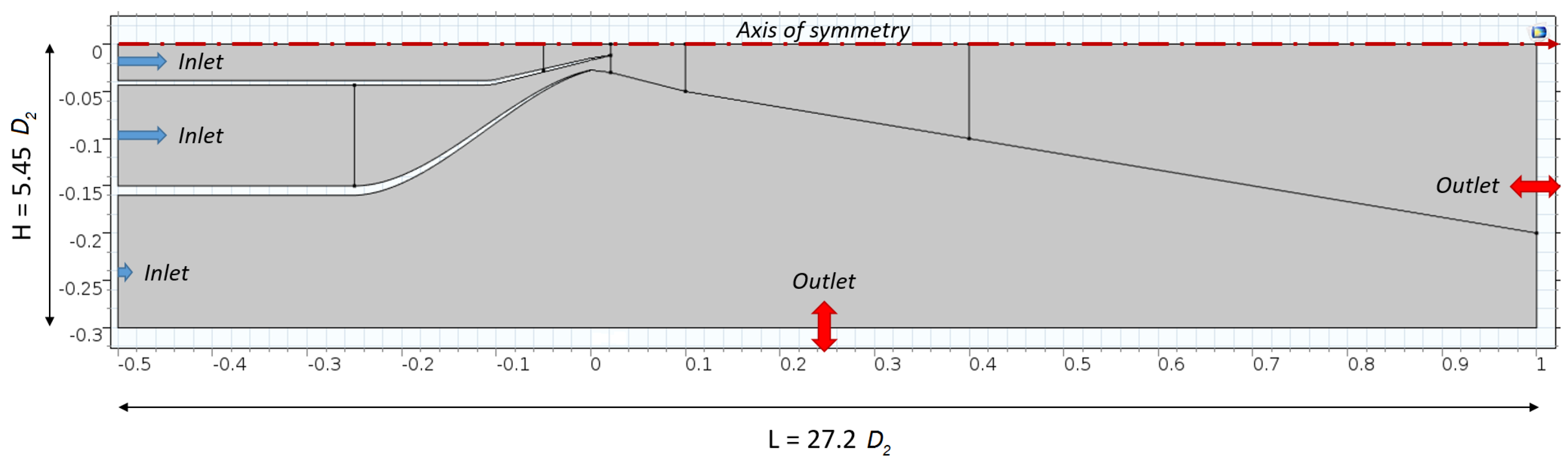
The simulation of the coaxial flow has been carried out using a RANS k- model. The computational domain is rectangular, extending 18.1 downstream and 9.1 upstream the nozzle in the axial direction, 5.5 in the radial direction. The ambient pressure is = 101,325 Pa, and the initial temperature was set to 293.15 K. Three inlet boundaries are present at the left of the domain, two boundaries inside the nozzles (, , K, ) and the third outside ( = 101,325 Pa, K, ). The outlet boundaries are the side and bottom edge of the domain with = 101,325 Pa. A no slip boundary condition is applied to all surfaces of the nozzle. A picture of the simulation domain is depicted in Figure 10. The simulations have been carried out varying only the total pressure at the two nozzle inlets.
5.3. Mesh Sensitivity
Initially, the COMSOL Multiphysics® 4.4 setting “Physics Controlled Mesh”, with the “Extremely fine” option, has been used. The software generated a free triangle elements mesh for the flow field and a boundary layer mesh on the walls. However, it has been assessed that this mesh was too coarse in the supersonic region because results showed no shock-cells in the jet. Consequently, another two meshes with higher resolution have been created and tested with the same pressure conditions. The elements maximum size of Mesh 3 is half of Mesh 2. In Figure 11, Mesh 1 and Mesh 2 near the nozzle exit region are compared. Details on the three meshes are shown in Table 3.
The three meshes have been compared in Figure 12 by plotting the Mach number extracted in the supersonic region over a straight line. The line is arbitrarily defined due to the fact that the maxima and minima of the Mach number in the jet do not lie on the centerline. The line, depicted in Figure 13a, is identified by the extremes A(0.32, 0.00) and B(0.24, 4.00), where the coordinates are non-dimensionalized by the secondary nozzle diameter . In this reference system, is the radial direction, the axial direction and the origin the intersection between the axis of symmetry and the exit plane of the secondary nozzle. The graph shows how the results for Mesh 1 have poor resolution in comparison with Mesh 2 and Mesh 3. The Mesh 2 is capable of calculating the first peak in accord with Mesh 3, but the amplitude for the other peaks is slightly different. In conclusion, because of the relatively high computational cost of Mesh 3, it has been decided to carry out all the simulations using the Mesh 2.
5.4. Results
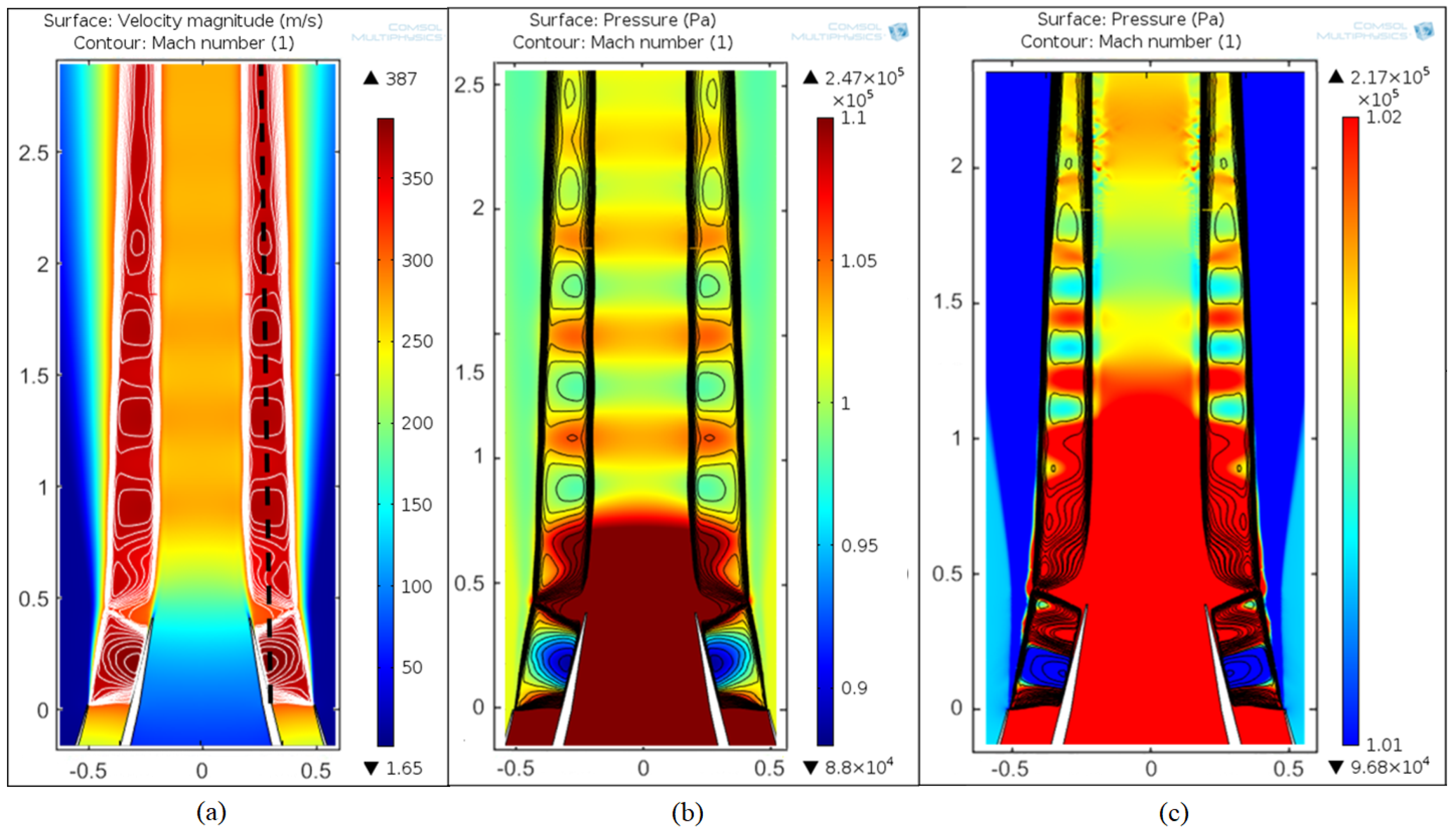
An annular shock-cells system is visible, starting from the exit of the secondary nozzle and surrounding the primary jet. At all the simulated conditions, a strong, conical, shock-wave is present, starting from the lip of the primary nozzle and refracting back into the flow when reaching the external shear layer (Figure 13). After the shock, the flow is locally subsonic, becoming again supersonic after a little distance, leading to the formation of annular shock-cells in the jet, between the internal shear layer and the external shear layer.
In Figure 13b, the pressure field shows a periodic pattern, due to the presence of the annular shock-cells. This causes also the velocity of the inner jet to be modulated according to the annular shock-cell topology. Reducing the total pressure, a progressive reduction on the length of the shock-cells is observable, similar to the single stream jets. For Cond. 07 (Figure 13c), it is possible to recognize the formation of a complete shock-cell also in the region between the external shear layer and the wall of the internal nozzle, while the formation of shock-cells in the jet is shifted downstream. This is caused by a destructive interaction between the oblique shock-wave and the expansion waves due to the underexpansion factor, confirmed by PIV measurements [15]. Further lowering the total pressure, shock-cells are still present between the secondary shear layer and the primary nozzle wall, while a large subsonic region is developing after the oblique shock-wave, becoming supersonic again much downstream the primary nozzle exit (Figure 14). No further shock-cells are visible in the simulations, but they are still present in the experiments [15].
One of the main result of this investigation is the deviation of the computed mass flow rates from the expected ones obtained using the isentropic relations. Especially for the primary nozzle, important differences have been found, with the mass flow rate lower by more than 30% for all the test conditions. The reason for this behavior can be attributed to the strong re-compression at the end of the primary nozzle, due to the conical shock-wave generated by the secondary stream. This analysis led to the choice to directly measure the primary mass flow rate with the orifice plate described in Section 2. Furthermore, the by-pass ratio is sensibly higher than initially estimated.
6. Commissioning
The commissioning phase aimed at two primary goals: firstly, the comparison of experimental results found in the literature and, secondly, the development of a testing methodology to be applied on the coaxial jet.
Unfortunately, very few experimental measurements on supersonic coaxial jets are present in the literature [13,18,19,20,21,22], and none of these examples matched our geometry and test conditions. For this reason, it has been decided to perform a test campaign using only the core nozzle to simulate a supersonic single stream jet. The aim is to compare the acoustic far field, using a microphone antenna, and the velocity field obtained through PIV. The facility would be considered commissioned if it is able to correctly replicate the results already available in the literature, for several test conditions.
A detailed analysis of the single stream jet is beyond the scope of this paper; therefore, only the PIV results obtained from the first test campaign and some of the acoustic results will be shown. The reader is addressed to Rubio Carpio [23] and Guariglia [15] for a more exhaustive analysis.
6.1. Experimental Setup
A vertical microphone polar array is located in the anechoic room comprised of 11 microphones, equally spaced to cover a range of polar angles from 30 to 130. The PIV optical bench, containing all the devices necessary to generate the laser light sheet and the cameras to record the images, is also placed inside the anechoic chamber. The laser head and its cooling system are kept outside of the room, since they are sources of spurious noise. A sketch of the final setup of the facility is shown in Figure 15. The nozzles used are the first set built, described in Section 3, with mm and mm for the primary and secondary jets, respectively. For this study, both the nozzles have been installed, but only the primary flow has been used. The seeding generator is a PivPart-45M, by PIVTEC Gmbh, composed of 45 Laskin nozzles, with 5 bar as the maximum outlet pressure. The manufacturer’s user manual [24] reported a peak in the particle size distribution function around m for vegetable oil. In this work, the seeding used was the industrial oil Shell Ondina-919. The Laser Extinction Spectroscopy [25] (LES) technique has been used at VKI by Mandon [26] to verify the seeding size distributions for this oil. The results show that the distribution is centered around 0.5 m for most of the tested conditions, thus suitable for this investigation.
6.2. Operating Conditions
Three measurement campaigns have been conducted. In the first one, PIV and microphones measurements have been performed synchronously, for the range of CNPR and Mach numbers indicated in Table 4. Unfortunately, the spectra retrieved from these measurements resulted in being altered for frequencies above ∼15 kHz. It has been verified a posteriori that the alteration came from the presence of the protective grid, which is normally mounted on this kind of microphones to protect the sensible membrane.
Following the manufacturer’s advise, acoustic measurements, without the protective grid, have been repeated and extended for lower and higher Mach numbers, as indicated in Table 4. The last acoustic measurement campaign has been executed using the Nozzle Set 2, for the sake of verifying the experimental repeatability and acoustic spectra similarity.
6.3. PIV Measurements
6.3.1. PIV Acquisition Procedure
Series of 1800 samples have been acquired for each flow case, with a sampling rate of 15 Hz. Consecutive fields can thus be assumed to be decorrelated. Taking as an example the work of André [27], the turbulence intensity in the mixing layer of the jet is estimated to be less than 20%. Assuming this value as an upper limit, it can be assumed that the number of samples taken allows one to have a error on the velocity mean value with a of confidence level [28].
6.3.2. PIV Equipment
The illumination is provided by laser pulses generated with a double-cavity Quantel CFR200 Nd:YAG system. This system provides a laser wavelength 532 nm (green), with a maximum energy of 200 mJ/pulse and a pulse duration of 12 ns.
After a transmission of approximately 3 m, the laser beam reaches the optical bench where the beam is reshaped as a laser sheet. The optical bench consists of two spherical lenses, one with focal length mm and the other one with mm, a cylindrical lens and a prism to rotate the laser beam. Being that a single lens with a proper focal length was unavailable, the combination of these two different spherical lenses fulfilled the need very well, guaranteeing the compactness of the optical test bench, to avoid disturbances in the acoustic measurements. After the cylindrical lens, the laser light sheet passes through the prism, where it is deviated 90 in order to reach the test section. The distance between the prism and the test section is about 1 m. This setup allowed obtaining a laser sheet of about 1 mm in thickness on a vertical plane containing the jet axis.
The recording system is composed of two LaVision Imager SX4M cameras (2360 × 1776 pixel2) located at a distance of 0.5 m from the jet axis. Acoustic tests have been carried out to ensure that at such a distance, the acoustic field emitted by the jet was not perturbed. The cameras are placed vertically in order to enlarge the total field of view in the axial direction of the jet, although a little overlap between the field of view of both cameras is set up in order to allow the construction of the final one by joining them.
Two Nikkor f/1.8 objectives of 50 mm in focal length are mounted with a focal number .
The cameras have been slightly de-focused to increase the size of the particles on the sensor, since they have been found to be at the limit of two pixels per particle. A posteriori, this is probably due to the particles’ diameter, which is smaller than 1 m according to the measurements of Mandon [26].
The final Field Of View (FOV) is shown in Figure 16. It has a total extension of 10.5× 4 (252 × 96 mm) with a resolution of 18 pixels/mm. A parametric study was carried out to choose the optimum separation time and seeding density for each case. The final separation times for each case are summarized in Table 4.
Before starting the data acquisition, the test chamber is filled with oil particles to seed the quiescent air surrounding the jet. Despite the different concentrations, this was sufficient to have a good signal to noise ratio in the jet entrainment region [15,23]. Figure 16a,b shows an instantaneous view of the seeded jet and a computed velocity field.
6.3.3. Image Processing
The image pre-processing and cross-correlation have been carried out with in-house PIV software [29,30,31]. WIDIM uses an iterative interrogation procedure with window shifting and deformation. Image interpolation at sub-pixel positions is performed by a standard three-point Gaussian function [32]. According to this, a 64 × 64 pixel2 initial interrogation window is used with two iterations, resulting in a final interrogation window of 16 × 16 pixel2, with 50% overlap. The spatial resolution is of one vector each of eight pixels (0.44 mm), i.e., 55 vectors across the single supersonic jet diameter. Those instantaneous flow fields with a signal to noise ratio lower than 1.5 or higher than 20 are filtered out.
6.3.4. Results: PIV
In this section, the results obtained from the PIV measurements are presented and compared with previous research. The main characteristics of the shock-cell pattern have been retrieved from the PIV measurements. Local Mach numbers can be computed from the PIV data assuming the total temperature does not change in the pipes, and it is equal to the reservoir one. With the further assumption of isentropic flow, the Mach number can be computed with the following formula [33]:
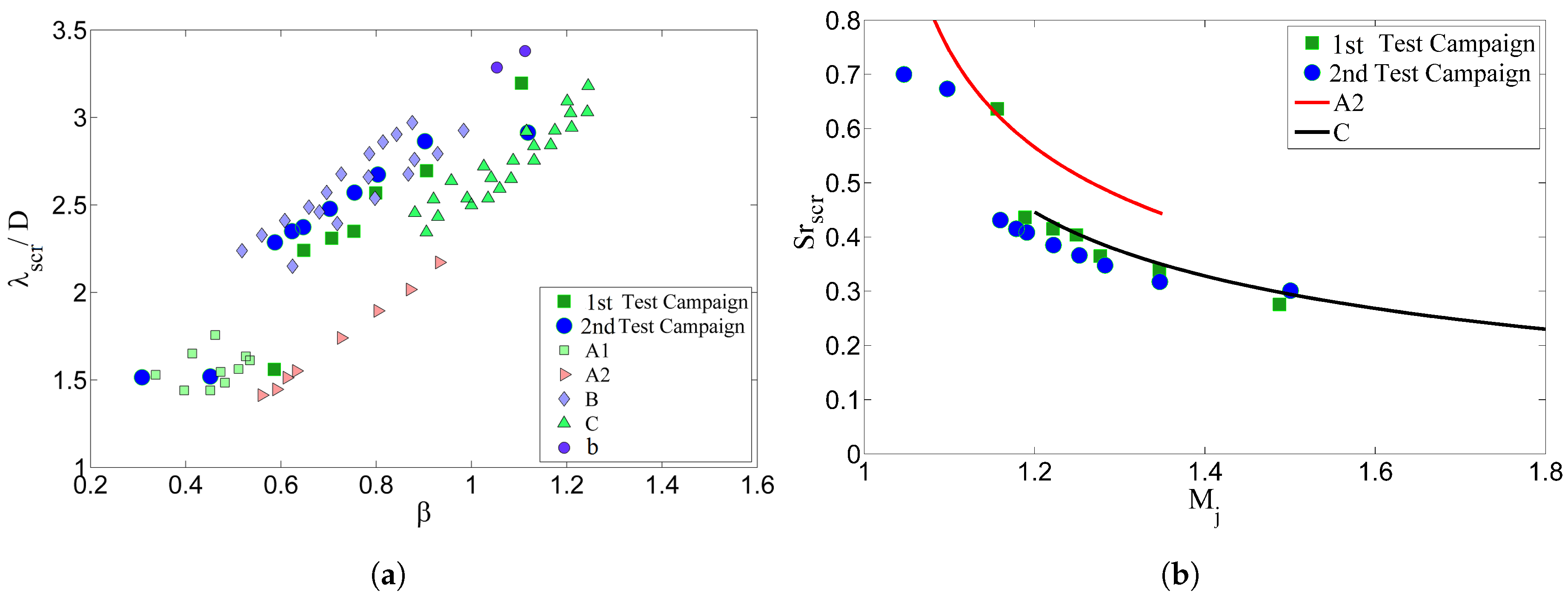
which is less and less valid as the shock-wave strength increases and in the shear layer, as the effect of entropy production. Pérez Arroyo, in his Large Eddy Simulations (LES) on a supersonic coaxial jet [34], found a difference <3% between the Mach number extracted from the simulation and calculated using this method [35]. An overview of the average velocity fields for all the tested condition is presented in Figure 17. The picture shows the progressive increment of the shock-cell length, but sudden reductions of the number of the shock-cells periodically occur. It was already known from the literature [27,36] that this is due to the effect of the screech mode change, which reduces the number of shock-cells by provoking large displacements of the plume. By comparing the screech tone frequency with the literature and by performing a cross-correlation analysis on the PIV fields, it has been assessed that for CNPR = 2.30, an axisymmetric screech mode (A2) is present; from CNPR = [2.40 2.50 2.60], there is the onset of a flapping mode (B); and finally, for CNPR = [2.7 2.96 3.67], there is an ongoing helical mode (C). Further information on the screech modes identification using cross-correlation analysis can be found in Guariglia [15].
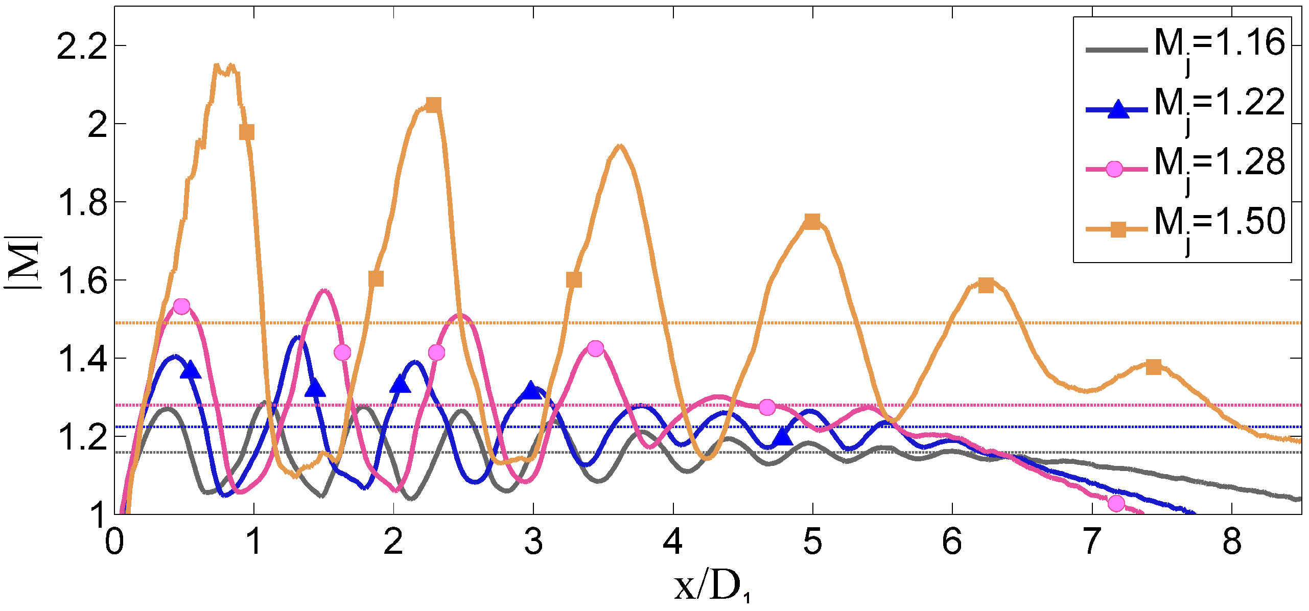
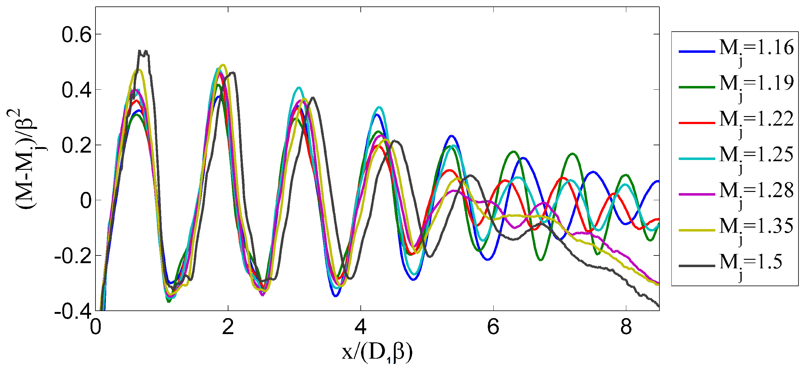
In Figure 18, the variation of the Mach number of the mean flow, in the center line, is shown. The amplitude of the fluctuations depends on the strength of the shocks present in the jet plume and thus on the off-design factor , defined as:
where is the fully-expanded Mach number for the jet and is the nozzle design Mach number (equal to one in this experiment). A method to collapse all the curves has been proposed by Savarese [37] for his non-screeching jet. The shock cell length appears to be proportional to , and the amplitude of the fluctuations is proportional the pressure mismatch, which, in turn, appears to be proportional to . Therefore, by dividing the length of the shock cells by the off design factor and the amplitude by , a collapse of all the curves is performed. The raw profiles and the collapsed ones are presented in Figure 18 and Figure 19.
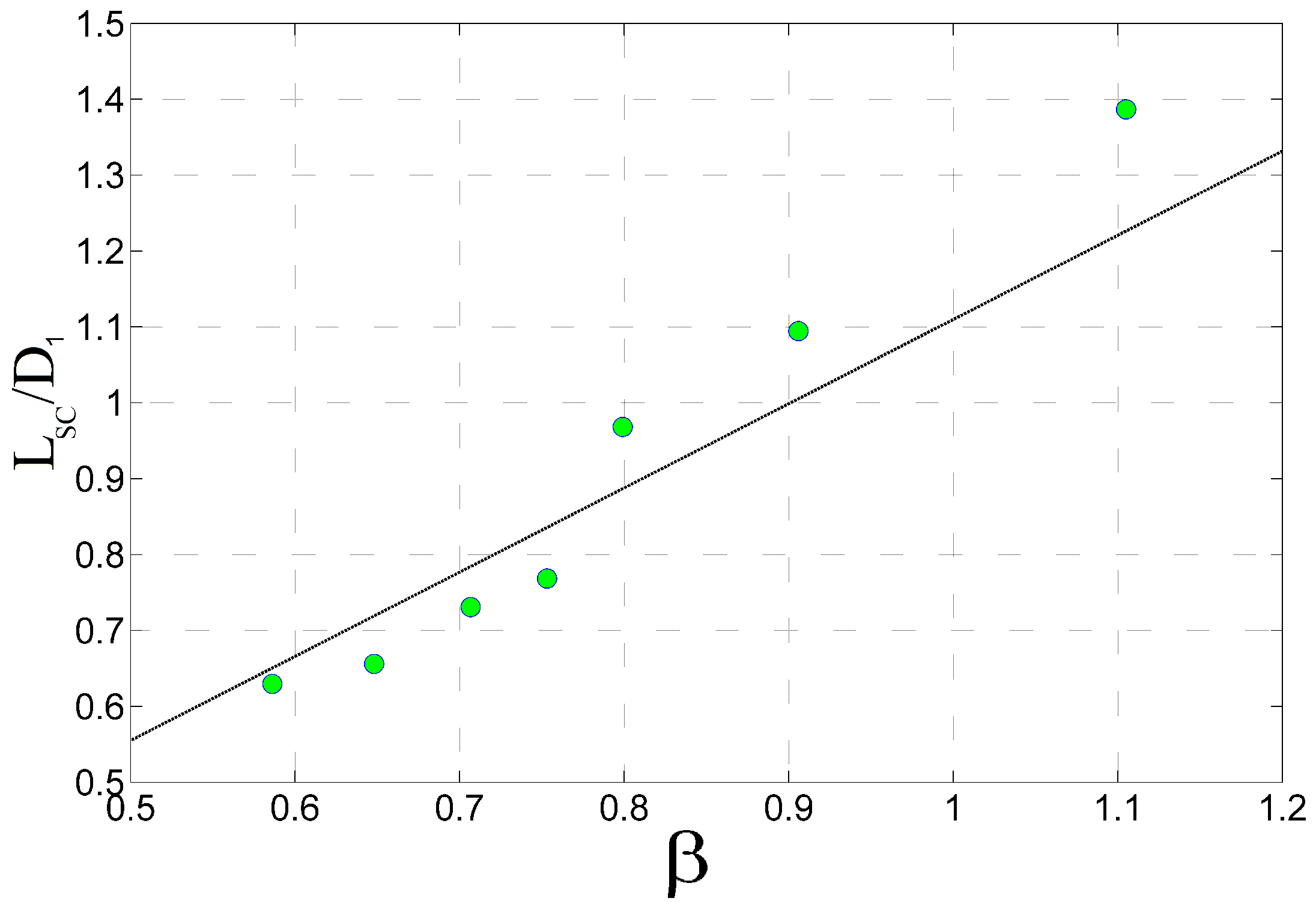
Overall, the behavior is acceptable for . Above this point, the curves lose coherence. The hypothesis is that the occurring screech is altering the shock-cells sequence, also by virtue of the fact that three different screech modes are present in the measurements. In Figure 20, the averaged shock-cell length has been compared with the semi-empirical relation proposed by Harper-Bourne and Fisher [38]. The mean value for every case is plotted. The measured data follow the proposed trend for all the cases. The sudden change at is attributed to a change of the jet screech mode.
6.4. Acoustic Measurements
A new microphone polar array has been designed to perform the acoustic measurements. Eleven microphones were positioned, covering an angular range from to (being the downstream direction), with a microphone every , at a distance of 1.32 m (55 ).
The microphones used are Bruel & Kjaer 4938, 1/4 inches in diameter with Bruel & Kjaer 2670 preamplifiers. Three Bruel & Kjaer NEXUS Type 2690-A microphone conditioners have been used to amplify and band-pass the signal.
6.4.1. Acquisition System
An NI 5751 14-bit A/D converter together with an NI PXIe-1073 chassis has been used to record the microphones’ signal. The sampling frequency is kHz. In all cases, the band-pass filter of the NEXUS system was set from 20 Hz to 100 kHz. The selected acquisition parameters for every test campaign are: acquisition time s, sampling frequency kHz, number of samples and frequency resolution Hz.
6.4.2. Data Processing
Welch’s Sound Pressure Level (SPL) of the signal is calculated. Welch’s SPL divides the whole acquired signal into segments of points using a Hanning window to limit spectral leakage. The final frequency resolution of the Welch averaged signal is Hz.
6.4.3. Results: Aeroacoustics
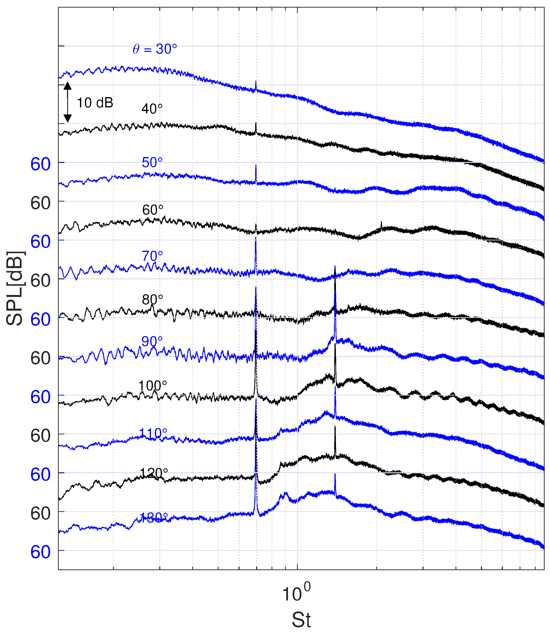
For the sake of brevity, only the cases with Nozzle Set 1 mounted, for CNPR = [2.00 2.26 2.30 3.67], are shown. For a description of the results at all the tested conditions, the reader is referred to Guariglia [15]. An overall view of the SPL measured by the eleven microphones, scaled at a distance , is displayed in Figure 21. The SPL, for each angle, is staggered for better readability.
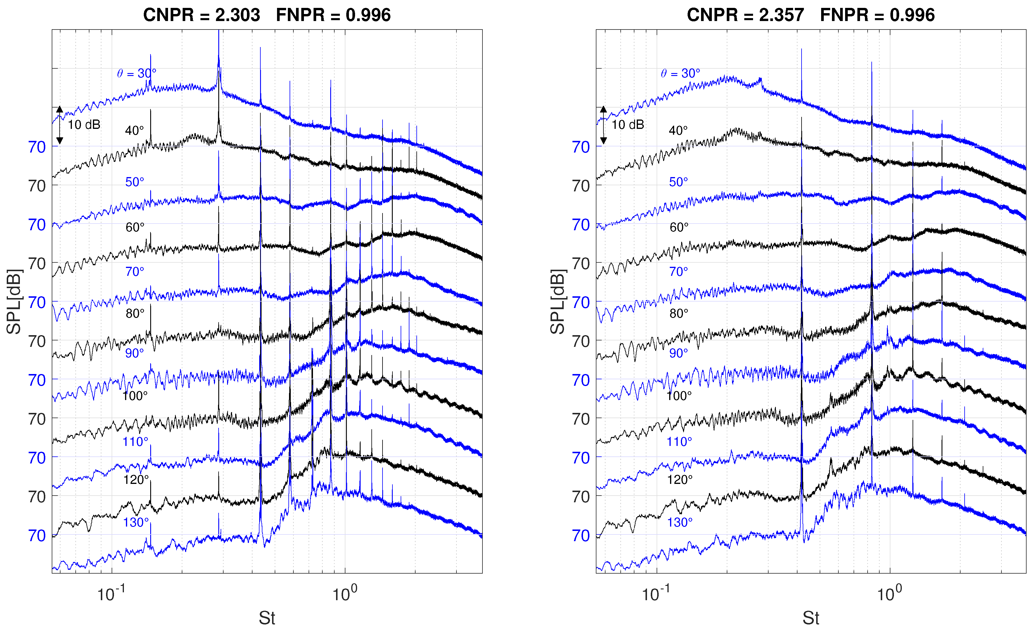
All the typical acoustic features of the shock-cell noise are present. The hump of broadband shock-cell noise is evident, and the frequency of the broadband spectral peak increases as the listener moves to downstream positions, as was already indicated by Tam [8]. The screech main tone and its harmonics are also present. As general behavior, the screech frequency decreases as the degree of underexpansion increases. This behavior has already been noticed in several publications [4,7,39]. At certain Mach numbers, the screech mode switches from axisymmetric (A2) to flapping mode (B) and then to helical mode (C), evidenced by a marked shift of the screech frequency when the switch is completed. In Figure 21 on the top right-hand side is shown a case where the jet experiences the transition between the modes (A2) and (B), and both screech tones are present at and , respectively.
Interestingly, in all conditions, many harmonics of the screech main tone can been counted (in some cases up to the 10th one). These harmonics express also a directivity pattern, intended as marked variation in the SPL at different angles, as pointed out already by Tam [40]. For the cases CNPR = [2.26 2.67], the presence of screech subharmonics, intended as tones at frequency lower than the main tone, has been recorded, together with harmonics of the subharmonic tones. Interestingly, these two cases correspond to when the screech mode is switching from one to another, which may suggest a causality effect. Apart from the study of Tam, little research has been conducted on this topic until now, mainly due to the difficulties in finding screeching jets with many harmonics, and no examples have been found in the literature on screech subharmonics. Further analysis, however, is beyond the scope of this paper, and thus, it will be addressed in future publications. Finally, when the the pressure ratio is sufficiently high to lead to the Mach disk formation, at CNPR = 4.00 , no screech is further encountered (with Nozzle Set 2 [15]).
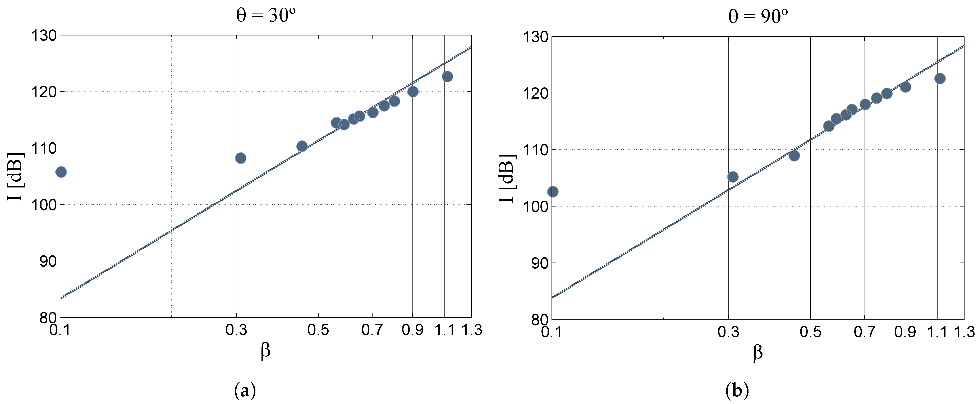
6.5. Comparison of the Sound Intensity Level
The Sound Intensity Level (SIL), defined as:
is a time averaged power flux, where T is the recording time, is the pressure fluctuation and and are the air speed of sound and density, respectively. The SIL is usually expressed in decibels [dB] by computing , where is the reference intensity. The integration of the SIL on a closed surface leads to the sound power level, which is sometimes found in the literature as SWL. Harper-Bourne and Fisher [38] found out that the shock-cell noise intensity is proportional to the fourth power of the off design parameter . Figure 22 illustrates the variation of the measured SIL vs. the off-design parameter for the microphones located at and . Measured data laying in the range , where the shock-cell noise is the main mechanism of noise generation, follow the aforementioned trend. Below this range, the shock-cells pattern is weak, and jet mixing noise becomes dominant, so Lighthill’s M8 law is retrieved.
The screech wavelength obtained in the measurements was compared with the literature for all the test cases. In Figure 23a, the results of the measurements are plotted together with the data gathered by Raman [41]. It was observed that all measured wavelengths lay in the point cloud retrieved in other research.
The data have also been compared with the correlations proposed by Ahuja [39] for the stable axisymmetric mode (A2) and the helical mode (C). The results are presented in Figure 23b, where the screech Strouhal number was calculated as . Most of the measured data lay near the helical mode (C) correlation, while one point lays in the stable axisymmetric mode (A2). The two points that remain far from any correlation curve belong to the unstable mode (A1) according to the data of Raman.
Summarizing, all the measurements performed in different test campaigns showed that the noise emitted by the supersonic jet in the FAST facility contains all the acoustic features of the shock-associated noise and are in agreement with previous literature results.
6.6. Nozzles Set Comparison
The acoustics results for the Nozzle Set 1 and Nozzle Set 2 have been compared. Spectra are non-dimensionalized by the Strouhal number and scaled as for distance . Figure 24 shows very good agreement among the two test campaigns, for both the BBSAN and the screech tones, in frequency and SPL. Interestingly, the pressure conditions for which there is the switch between the axisymmetric and flapping screech modes is not the same for the two nozzle. The onset of the switch has been determined by monitoring the spectra “live” during the experiments and finely increasing the CNPR until the set of subharmonics first appear. For the larger nozzle, this occurs around CNPR = 2.26 (shown in Figure 21), while for the smaller nozzle at CNPR = 2.30 (Figure 25 on the left). In the same way, it has been assessed that the switch is complete around CNPR = 2.30 for the larger nozzle (Figure 21 bottom left) and CNPR = 2.36 for the smaller one (Figure 25 on the right). This behavior does not change even when starting from CNPR = 2.40 and finely decreasing the pressure. This may suggest a dependency different from the Strouhal number. This aspect, however, has not been investigated further.
6.7. Preliminary Dual Stream Jet Results
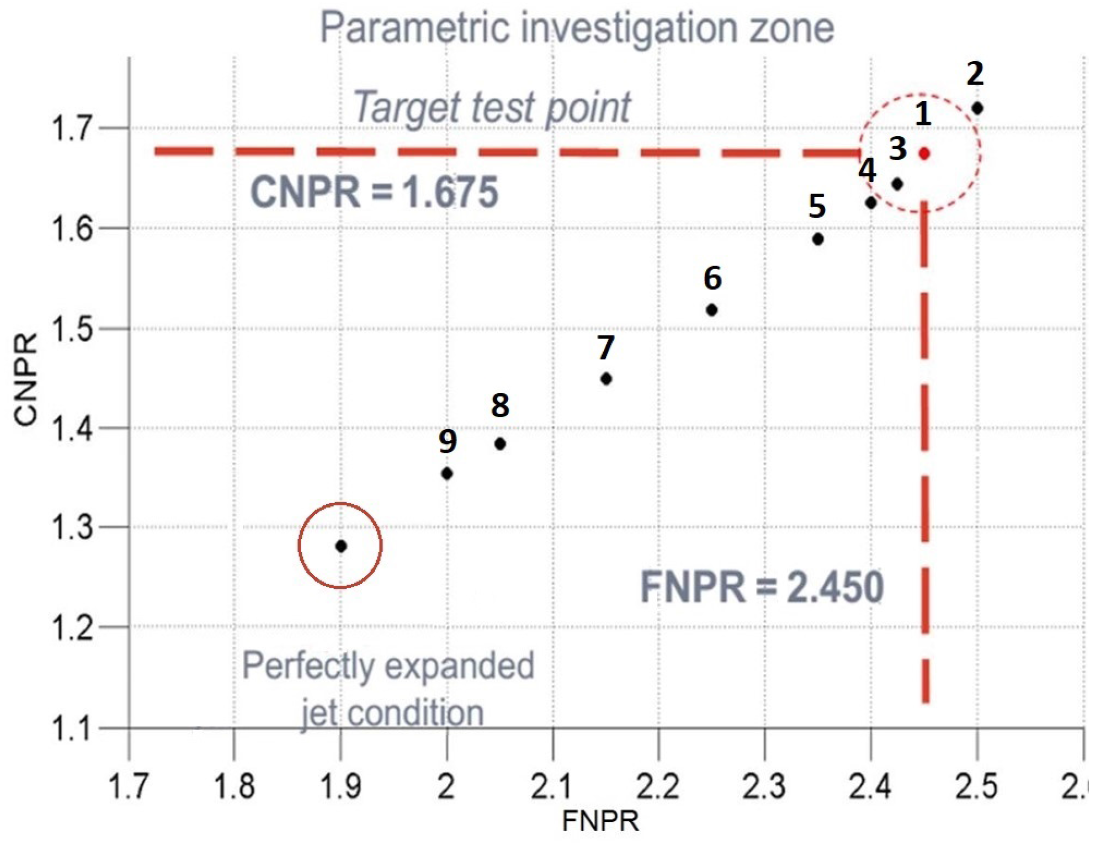
Following the single stream campaign, the dual stream nozzle has also been commissioned, and experiments have been carried out with Nozzle Set 2 for FNPR = 2.450 and CNRP = 1.675 (Condition 01 in Table 2). Preliminary results are shown, leaving a more detailed analysis for a future publication.
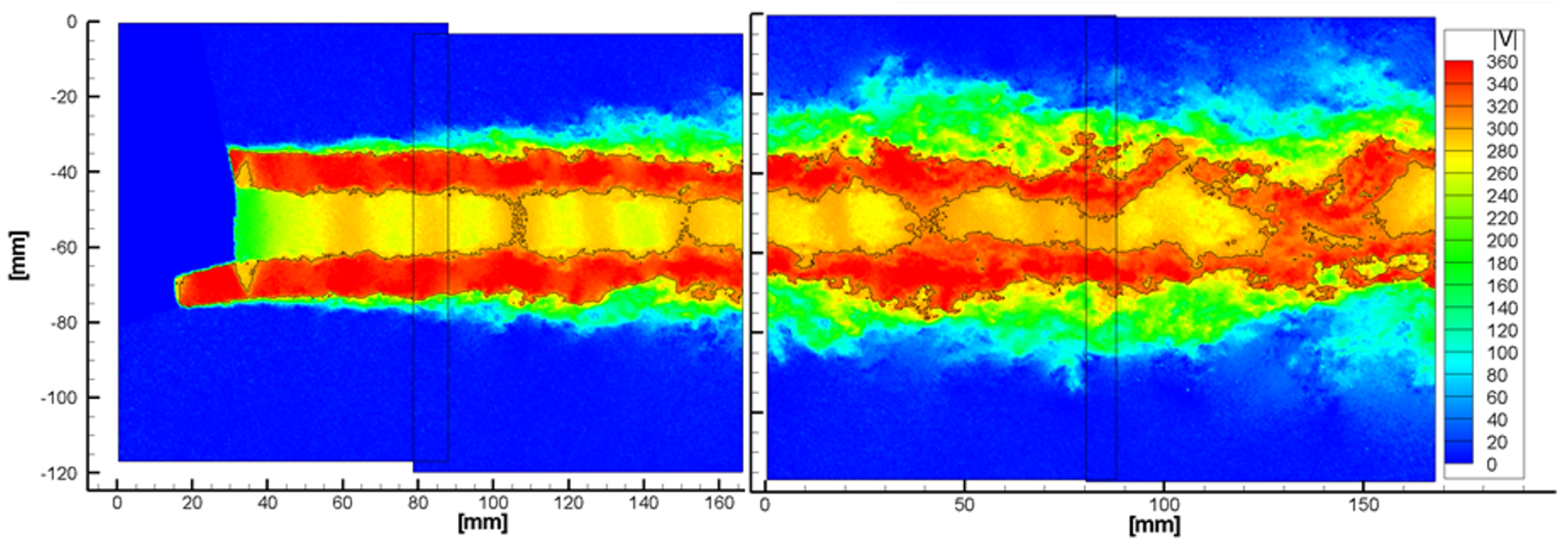
The experimental setup for the coaxial jet experiment does not differ significantly from the single jet. The main issue is posed by the longer extension of the jet itself, imposing a compromise between resolution and spatial correlation. The adopted solution consists of using the cameras side by side covering half of the supersonic extension (estimated through CFD), then measuring all points in the test matrix, then moving the laser sheet and the cameras to cover the second half of the supersonic region. The total length of the investigation zone spans for in the axial direction and in the radial direction. A second set of measurements investigates a specific portion of the jet with higher resolution. A sketch of the field of views is presented in Figure 26. An example of instantaneous flow field is depicted in Figure 27, while an averaged field of view is shown in Figure 28.
The magnification factor is 0.05 mm/pixel. The pre-processing, cross-correlation and post-processing have been carried out with VKI in-house software [29,30,31], similarly to the single jet. Based on the previous experience, the seeding generator has been used at its maximum capability. For the first investigation area, near the nozzle exit, the laser pulse separation time has been set to = 1 s for all the test conditions. For Condition 1 only, = 0.4 s and = 2 s have been used, as well, in order to verify the effects on the Signal-to-Noise Ratio (SNR) on the jet core (faster region) and on the shear layer (slower region). This assessment confirms that the separation time = 1 s is the best compromise between SNR and accuracy of the measurement [15]. For the second area, downstream the first area, the separation time has been increased to = 1.5 s. The final windows’ correlation, after two-step refinement and deformation is 12 × 12 pixels with 50% overlap, corresponding to a spatial resolution of ca. 0.60 × 0.60 mm and a vector resolution of ca. 150 vectors/.
The aeroacoustic measurements have been carried out using the same microphone antenna used for the single stream jet. Distance has been set to , with the acquisition frequency kHz, while the number of acquired samples is . From a qualitative point of view, dual stream spectra are similar to the single stream ones, with the exception that fewer screech tones are observable. An example is given in Figure 29.
7. Conclusions and Perspectives
A new facility to study supersonic coaxial jets has been designed and built for the investigation of shock-cell noise on single and dual stream jets. An innovative coaxial silencer has been realized to eliminate spurious noise from the piping and valve system. The main advantage of this configuration is to mitigate the aerodynamic interference between the inner duct and the outer ducts. The U-turn shape combined with the presence of stainless steel wool leads to an effective sound damping, evaluated by means of acoustic simulations. The nozzle geometry has been verified with RANS simulations, evaluating nine test conditions. The results evidence a complex flow pattern, with a conical shock-wave present at the end of the primary nozzle. This conical shock causes a sensible reduction of the primary mass flow rate, by creating an over-pressurized zone downstream the primary nozzle. This observation justifies the installation of a mass flow meter for the primary stream to directly measure the mass flow rate.
The FAST facility has been commissioned by performing experiments on a supersonic single stream jet in underexpanded conditions and comparing the results with the literature. Several CNPR conditions have been investigated using PIV with microphones mounted on a polar antenna. The velocity fields show the expected shock-cells pattern, with the shock-cell length increasing with the CNPR. The evolution of the mean shock cell length with the design parameter is in agreement with the semi-empirical correlation proposed by Harper Bourne and Fisher.
Acoustic measurements have been compared with the literature, finding good qualitative and quantitative agreement in terms of the sound intensity level trend and screech mode characteristics. Harmonics of the screech, up to the 10th one, have been found in all the conditions where screech was present. In two cases, the presence of many subharmonics of the main screech frequency appears as a specific feature of the present facility. It has been evidenced how such subharmonics are present only in cases when the jet is is switching between two screech modes, suggesting a causality effect for the phenomenon. In all cases, harmonics and subharmonics exhibit a directivity pattern, intended as the marked change of the SPL with the observer angle. Further research on this topic is envisaged, at first by comparing the directivity patterns with the model developed by Tam and secondly by performing wavelet analysis of the acoustic signal in the cases when the jet is exhibiting the subharmonic tones. In this way, it should be possible to determine if the phenomenon is at least continuous or intermittent.
The acoustic measurements for the two manufactured nozzle have been compared, showing a very good match on the SPL-St plane, at a relative distance of . This confirms the repeatability of the measurements also in light of the spectral self-similarity for supersonic underexpanded jets. The screech main tones and harmonics coincide in the Strouhal number for all cases, and the screech harmonics’ amplitudes and directivity patterns also maintain reasonably good agreement with the literature in all test conditions.
Finally, preliminary experiments on the dual stream jet have been performed, showing the capability of the facility to reach the nominal conditions also with the secondary flow.
In conclusion, the FAST facility and the experimental methodology have been validated, demonstrating how the rig is capable of fulfilling the objectives for which it has been designed.
Acknowledgments
Fulvio Stella from Università degli Studi di Roma “La Sapienza” (IT) is acknowledged for the support and mentoring during these studies. For the financial support, the European Commission is gratefully acknowledged, provided in the framework of the FP7 Marie Curie ITN (Initial Training Network) Project AeroTraNet2 (Grant Agreement No. 317142).
Author Contributions
Daniel Guariglia and Christophe Schram designed the FAST facility and supervised the manufacturing and installation process. Daniel Guariglia performed the CFD and acoustic simulations. Daniel Guariglia and Alejandro Rubio Carpio conceived of the experimental setup, performed the measurement and post-processed the data. Daniel Guariglia wrote the paper, Alejandro Rubio Carpio and Christophe Schram reviewed it. Christophe Schram supervised the whole project as the Principal Investigator.
Conflicts of Interest
The authors declare no conflict of interest.
Abbreviations
The following abbreviations are used in this manuscript:
| A | Area, m |
| c | Speed of sound, m/s |
| D | Diameter, m |
| f | Frequency, Hz |
| Focal number | |
| h | Height, m |
| I | Sound intensity level, W/m |
| l | Length, m |
| L | Length, m |
| m | Mass, kg |
| Mass flow rate, kg/s | |
| M | Mach number |
| N | Number of samples |
| p | Pressure, Pa |
| P | Power, W |
| r | Radius, m |
| Strouhal number, | |
| t | Thickness, m |
| T | Temperature, K |
| Velocity vector, m/s | |
| Acronyms | |
| BBSAN | Broadband Shock-Associated Noise |
| BPR | By-Pass Ratio |
| CAA | Computational AeroAcoustics |
| CAD | Computer Aided Design |
| CFD | Computational Fluid Dynamics |
| CNPR | Core Nozzle Pressure Ratio |
| FAST | Free jet AeroacouSTic laboratory |
| FNPR | Fan Nozzle Pressure Ratio |
| FOV | Field of View |
| LES | Laser Extinction Spectroscopy |
| LES | Large Eddy Simulations |
| RANS | Reynolds Averaged Navier–Stokes |
| PIV | Particle Image Velocimetry |
| SIL | Sound Intensity Level |
| SPL | Sound Pressure Level |
| SWL | Sound Power Level |
| TL | Transmission loss |
| VKI | von Karman Institute |
| Subscripts | |
| 0 | Stagnation condition |
| 1 | Primary nozzle |
| 2 | Secondary nozzle |
| ∞ | Free stream condition |
| a | Ambient condition |
| Canister holding the acoustic absorbent material | |
| d | Design condition |
| Duct section between the nozzleand the silencer | |
| Equivalent | |
| Input | |
| Measured internally | |
| j | Fully expanded |
| Maximum | |
| Output | |
| Reference value | |
| s | Sampling |
| Shock-cell | |
| Screech | |
| Silencer | |
| Stainless steel wool | |
| Symbols | |
| Angle, ° | |
| Off-design factor | |
| Correction to the reactance | |
| Frequency resolution, Hz | |
| Time interval, s | |
| Wavelength, m | |
| Dynamic viscosity, Pa·s | |
| Area porosity | |
| Angle, ° | |
| Flow resistance |
References
- Powell, A. On the Mechanism of Choked Jet Noise. Proc. Phys. Soc. Sect. B 1953, 66, 1039. [Google Scholar]
- Tanna, H. An experimental study of jet noise part II: Shock associated noise. J. Sound Vib. 1977, 50, 429–444. [Google Scholar]
- Harper-Bourne, M.; Fisher, M. The noise from shock waves in supersonic jets. In Proceedings of the AGARD Conference on Noise Mechanisms, Brussels, Belgium, 19–21 September 1973. [Google Scholar]
- Tam, C.; Tanna, H. Shock associated noise of supersonic jets from convergent-divergent nozzles. J. Sound Vib. 1982, 81, 337–358. [Google Scholar]
- Norum, T.D.; Seiner, J.M. Broadband Shock Noise from Supersonic Jets. AIAA J. 1982, 20, 68–73. [Google Scholar]
- Norum, T.D.; Seiner, J.M. Measurements of Mean Static Pressure and Far Field Acoustics of Shock-Containing Supersonic Jets; NASA TM84521d; NASA Langley Research Center: Hampton, VA, USA, 1982.
- Tam, C.; Seiner, J.; Yu, J. Proposed relationship between broadband shock associated noise and screech tones. J. Sound Vib. 1986, 110, 309–321. [Google Scholar]
- Tam, C. Broadband shock-associated noise of moderately imperfectly expanded supersonic jets. J. Sound Vib. 1990, 140, 55–71. [Google Scholar]
- Colonius, T.; Lele, S.K. Computational aeroacoustics: Progress on nonlinear problems of sound generation. Prog. Aerosp. Sci. 2004, 40, 345–416. [Google Scholar]
- Lele, S.K.; Mendez, S.; Ryu, J.; Nichols, J.; Shoeybi, M.; Moin, P. Sources of high-speed jet noise: Analysis of LES data and modeling. Procedia Eng. 2010, 6, 84–93. [Google Scholar]
- Nichols, J.; Ham, F.; Lele, S.; Moin, P. Prediction of supersonic jet noise from complex nozzles. Cent. Turbul. Res. Annu. Res. Briefs 2011, 3–14. [Google Scholar]
- Shur, M.L.; Spalart, P.R.; Strelets, M.K. Noise Prediction for Underexpanded Jets in Static and Flight Conditions. AIAA J. 2011, 49, 2000–2017. [Google Scholar]
- Viswanathan, K. Parametric study of noise from dual-stream nozzles. J. Fluid Mech. 2004, 521, 36–68. [Google Scholar]
- Miller, S.; Morris, P. The Prediction of Broadband Shock-Associated Noise from Dualstream and Rectangular Jets Using RANS CFD. In Aeroacoustics Conferences; American Institute of Aeronautics and Astronautics: Reston, VA, USA, 2010. [Google Scholar]
- Guariglia, D. Shock-Cell Noise Investigation on a Subsonic/Supersonic Coaxial Jet. Ph.D. Thesis, Università degli Studi di Roma “La Sapienza”, Roma, Italy, 2017. [Google Scholar]
- COMSOL Multiphysics®5.0 Acoustic Module User Guide; COMSOL Inc.: Stockholm, Sweden, 2014.
- Givoli, D.; Neta, B. High-order non-reflecting boundary scheme for time-dependent waves. J. Comput. Phys. 2003, 186, 24–46. [Google Scholar]
- Tanna, H.; Brown, W.; Tam, C. Shock associated noise of inverted-profile coannular jets, part I: Experiments. J. Sound Vib. 1985, 98, 95–113. [Google Scholar]
- Tam, C.; Tanna, H. Shock associated noise of inverted-profile coannular jets, part II: Condition for minimum noise. J. Sound Vib. 1985, 98, 115–125. [Google Scholar]
- Tam, C.; Tanna, H. Shock associated noise of inverted-profile coannular jets, part III: Shock structure and noise characteristics. J. Sound Vib. 1985, 98, 127–145. [Google Scholar]
- Debiasi, M.; Papamoschou, D. Noise from imperfectly expanded supersonic coaxial jets. AIAA J. 2001, 39, 388–395. [Google Scholar]
- Bhat, T.; Ganz, U.; Guthrie, A. Acoustic and Flow-Field Characteristics of Shock-cell Noise from Dual Flow Nozzles. In Aeroacoustics Conferences; American Institute of Aeronautics and Astronautics: Reston, VA, USA, 2005. [Google Scholar]
- Rubio Carpio, A. Experimental Investigation on Shock-Cell Noise; Research Master Report; von Karman Institute for Fluid Dynamics: Rhode-Saint-Genèse, Belgium, 2016. [Google Scholar]
- PIVTEC–GmbH. Aerosol Generator PivPart45-M Series User Manual; PIVTEC–GmbH: Gottingen, Germany, 2013. [Google Scholar]
- Horváth, I. Development and Applications of the Light Extinction Spectroscopy Technique for Characterizing Small Particles. Ph.D. Thesis, Université Libre de Bruxelles, Bruxelles, Belgium, 2015. [Google Scholar]
- Mandon, J.B. Acoustic Dumping by Spray Curtains. Master’s Thesis, von Karman Institute, Rhode-Saint-Genèse, Belgium, 2016. [Google Scholar]
- André, B. Etude Experimentale de L’Effet du vol sur le Bruit de Choc de Jets Supersoniques Sous-Detendus. Ph.D. Thesis, Ecole Centrale de Lyon, Ecully, France, 2012. [Google Scholar]
- Horvath, I. Extreme PIV Applications: Simultaneous and Instantaneous Velocity and Concentration Measurements on Model and Real Scale Car Park Fire Scenarios. Ph.D. Thesis, Université libre de Bruxelles, Bruxelles, Belgium, 2012. [Google Scholar]
- Horvath, I. PIV Image Pre-Processing by Tucsok; Von Karman Institute: Rhode-Saint-Genèse, Belgium, 2011. [Google Scholar]
- Scarano, F.; Riethmuller, L.M. Iterative multigrid approach in PIV image processing with discrete window offset. Exp. Fluids 1999, 26, 513–523. [Google Scholar]
- Horvath, I. PIV Data Processing by Rabon; Von Karman Institute: Rhode-Saint-Genèse, Belgium, 2011. [Google Scholar]
- Stanislas, M.; Okamoto, K.; Kahler, C.J.; Westerweel, J.; Scarano, F. Main results of the third international PIV Challenge. Exp. Fluids 2008, 45, 27–71. [Google Scholar]
- André, B.; Castelain, T.; Bailly, C. Investigation of the mixing layer of underexpanded supersonic jets by particle image velocimetry. Int. J. Heat Fluid Flow 2014, 50, 188–200. [Google Scholar]
- Pérez Arroyo, C.; Daviller, G.; Boussuge, J.F.; Arieau, C. Large Eddy Simulation of Shock-Cell Noise From a Dual Stream Jet. In Proceedings of the 22nd AIAA/CEAS Conference, Lyon, France, 30 May–1 June 2016; American Institute of Aeronautics and Astronautics (AIAA): Reston, VA, USA, 2016. [Google Scholar]
- Pérez Arroyo, C. (CERFACS, Toulouse, France). Private communication, 2016. [Google Scholar]
- Savarese, A. Experimental Study and Modelling of Shock Cell Noise. Ph.D. Thesis, Ecole Nationale Superieure d’Ingegneurs de Poitiers, Poitiers, France, 2014. [Google Scholar]
- Savarese, A.; Jordan, P.; Girard, S.; Collin, E.; Porta, M.; Gervais, Y. Experimental study of shock-cell noise in underexpanded supersonic jets. In Proceedings of the 19th Aeroacoustics Conferences, Berlin, Germany, 27–29 May 2013; American Institute of Aeronautics and Astronautics: Reston, VA, USA, 2013. [Google Scholar]
- Harper-Bourne, M.; Fisher, M.J. The Noise from Shock waves in Supersonic Jets. In Proceedings of the No.131 of the AGARD Conference on Noise Mechanisms, Brussels, Belgium, 19–21 September 1973; pp. 11-1–11-14. [Google Scholar]
- Massey, K.C.; Ahuja, K.K. Screech Frequency Prediction in Light of Mode detection and Convection Speed Measurements for Heated Jets. In Proceedings of the 3rd AIAA/CEAS Aeroacoustics Conference, Atlanta, GA, USA, 12–14 May 1997; American Institute of Aeronautics and Astronautics: Reston, VA, USA, 1997; pp. 315–324. [Google Scholar]
- Tam, C.K.W.; Parrish, S.A.; Viswanathan, K. Harmonics of Jet Screech Tones. AIAA J. 2014, 52, 2471–2479. [Google Scholar]
- Raman, G. Advances in understanding supersonic jet screech: Review and perspective. Prog. Aerosp. Sci. 1998, 34, 45–106. [Google Scholar]
Figure 1.
Sketch of the FAST final configuration.

Figure 2.
CAD drawing of the air supply system.
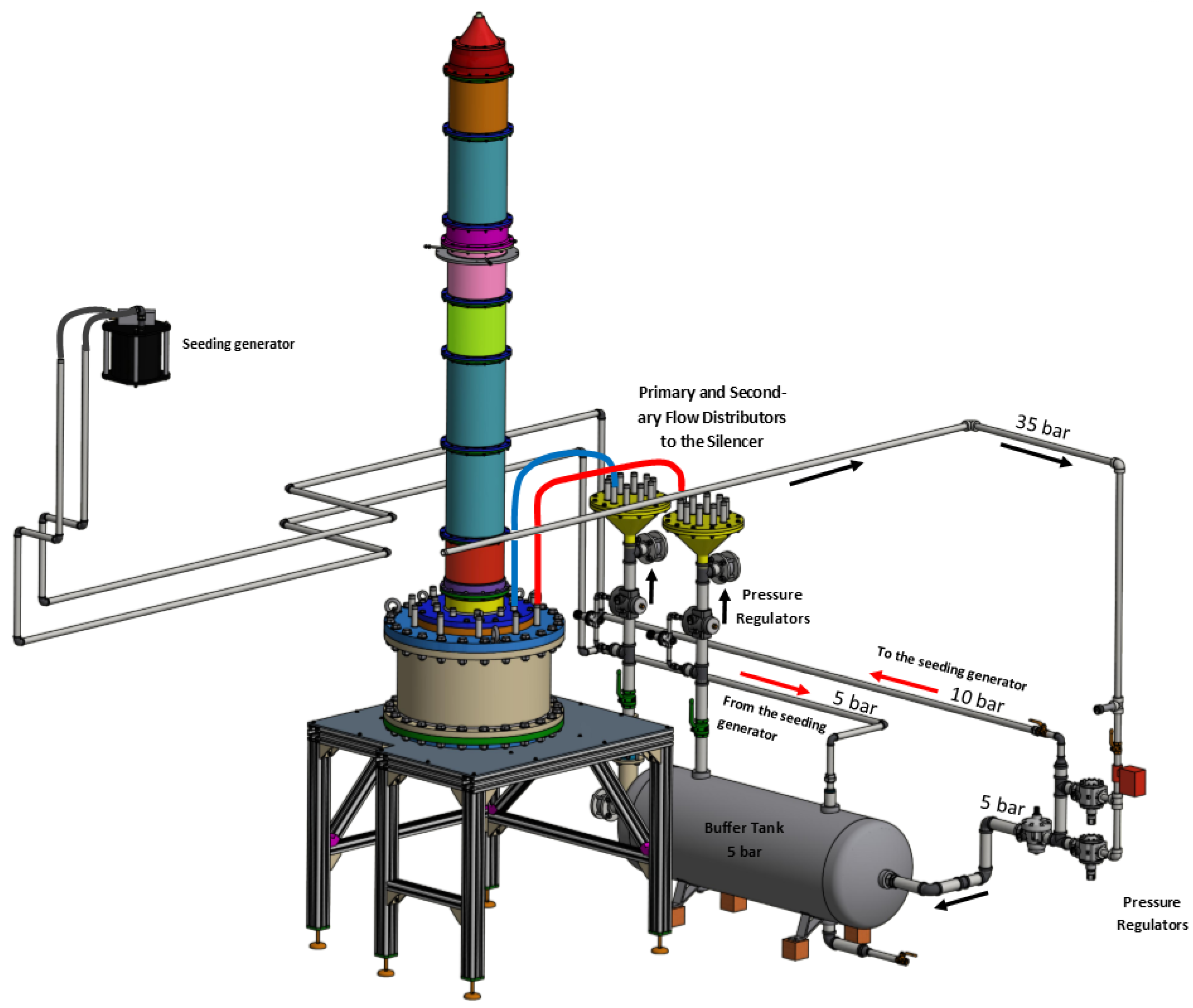
Figure 3.
(a) Section of the silencer and coaxial ducts. (b) Detail of the ducts. The pressure tap of the primary flow is located below the grids of the secondary one, thus decreasing the risk of introducing vortex shedding noise. (c) Detail of the coaxial silencer. The clean passage areas for the primary and secondary flow are colored in cyan and red, respectively. The gray zones represents the acoustic absorbent material. The overall dimensions are m, m, weight kg.
Figure 4.
CAD drawing of the coaxial nozzles sets. Dimensions are in mm. (a) Nozzle Set 1, used for CFD and single stream jet experiments; (b) Nozzle Set 2, used for single and dual stream experiments; (c) 3D view.
Figure 4.
CAD drawing of the coaxial nozzles sets. Dimensions are in mm. (a) Nozzle Set 1, used for CFD and single stream jet experiments; (b) Nozzle Set 2, used for single and dual stream experiments; (c) 3D view.

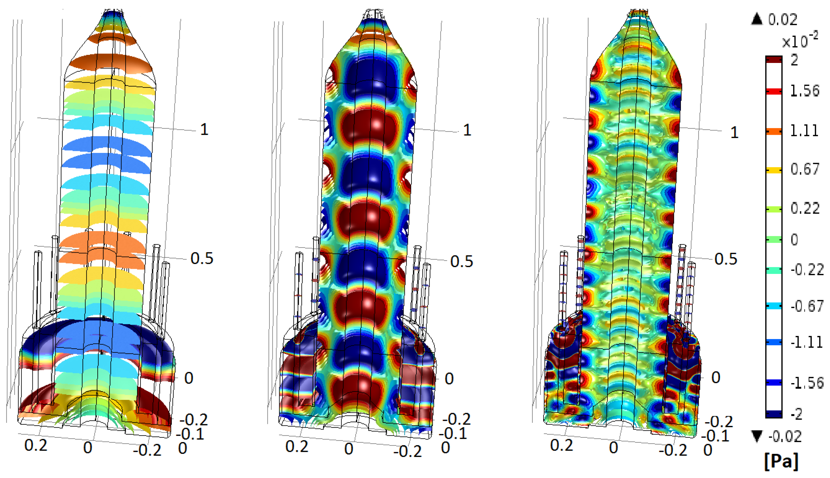
Figure 5.
Acoustic pressure field isosurfaces in the primary flow circuit at 570 Hz (left), 1840 Hz (center) and 5000 Hz (right). The scale enhances the modes visualization, which otherwise would be very faint at full scale.
Figure 5.
Acoustic pressure field isosurfaces in the primary flow circuit at 570 Hz (left), 1840 Hz (center) and 5000 Hz (right). The scale enhances the modes visualization, which otherwise would be very faint at full scale.
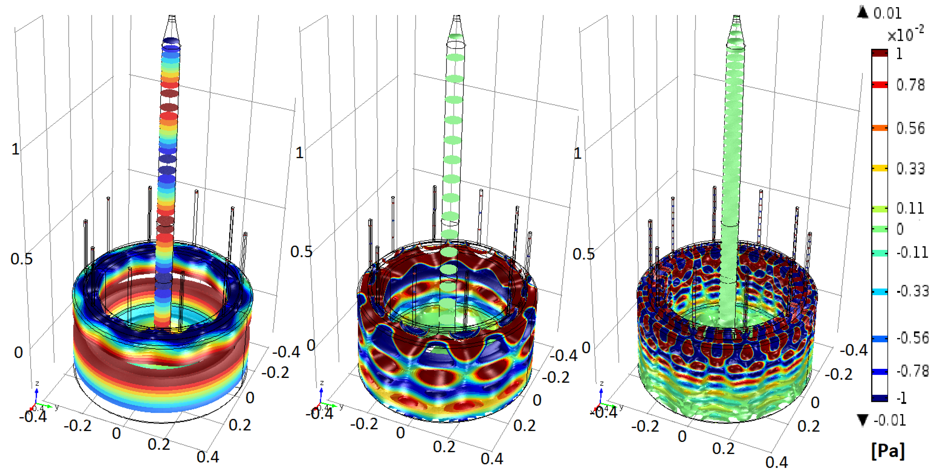
Figure 6.
Acoustic pressure field isosurfaces in the secondary flow circuit at 480 Hz (left), 2050 Hz (center) and 4790 Hz (right). The scale enhances the modes visualization that otherwise would be very faint at full scale.
Figure 6.
Acoustic pressure field isosurfaces in the secondary flow circuit at 480 Hz (left), 2050 Hz (center) and 4790 Hz (right). The scale enhances the modes visualization that otherwise would be very faint at full scale.

Figure 7.
Transmission loss of the silencer for the primary flow.
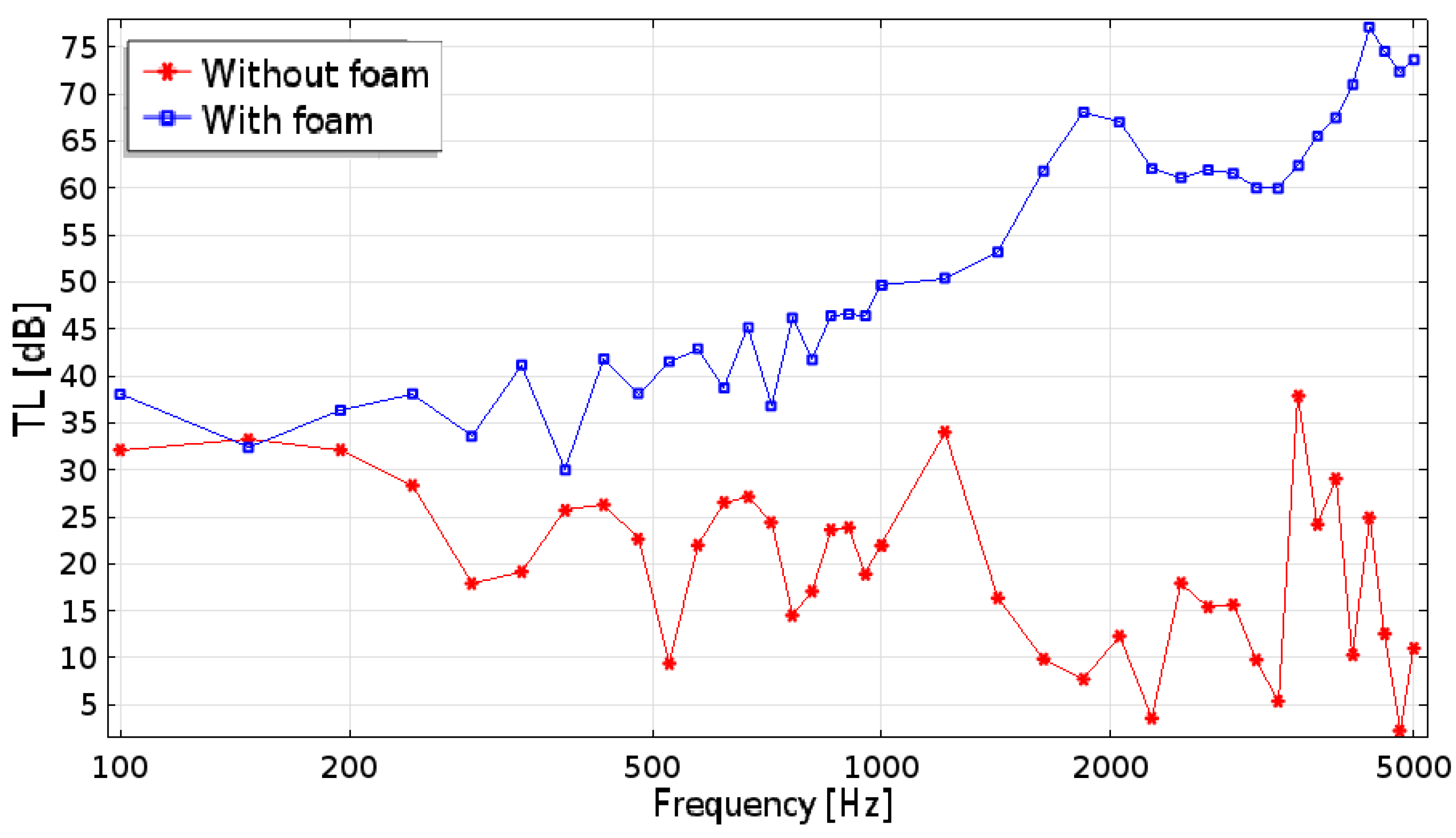
Figure 8.
Transmission loss of the silencer for the secondary flow.

Figure 9.
The parametric investigation chart. The perfectly expanded condition is shown as a reference, but it is not the subject of investigation.
Figure 9.
The parametric investigation chart. The perfectly expanded condition is shown as a reference, but it is not the subject of investigation.

Figure 10.
Example of the computational domain. Dimensions in m.

Figure 11.
Comparison of “Physics Controlled” Mesh 1 and “User-defined” Mesh 2.
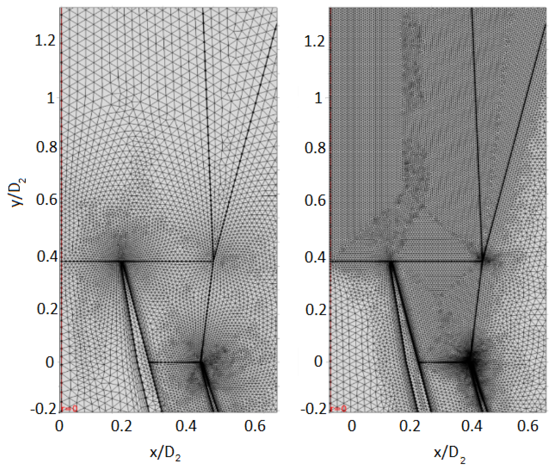
Figure 12.
Comparison of“Physics Controlled” Mesh 1 and “User-defined” Mesh 2 and Mesh 3. Data have been extracted from the dashed line in Figure 13.
Figure 12.
Comparison of“Physics Controlled” Mesh 1 and “User-defined” Mesh 2 and Mesh 3. Data have been extracted from the dashed line in Figure 13.
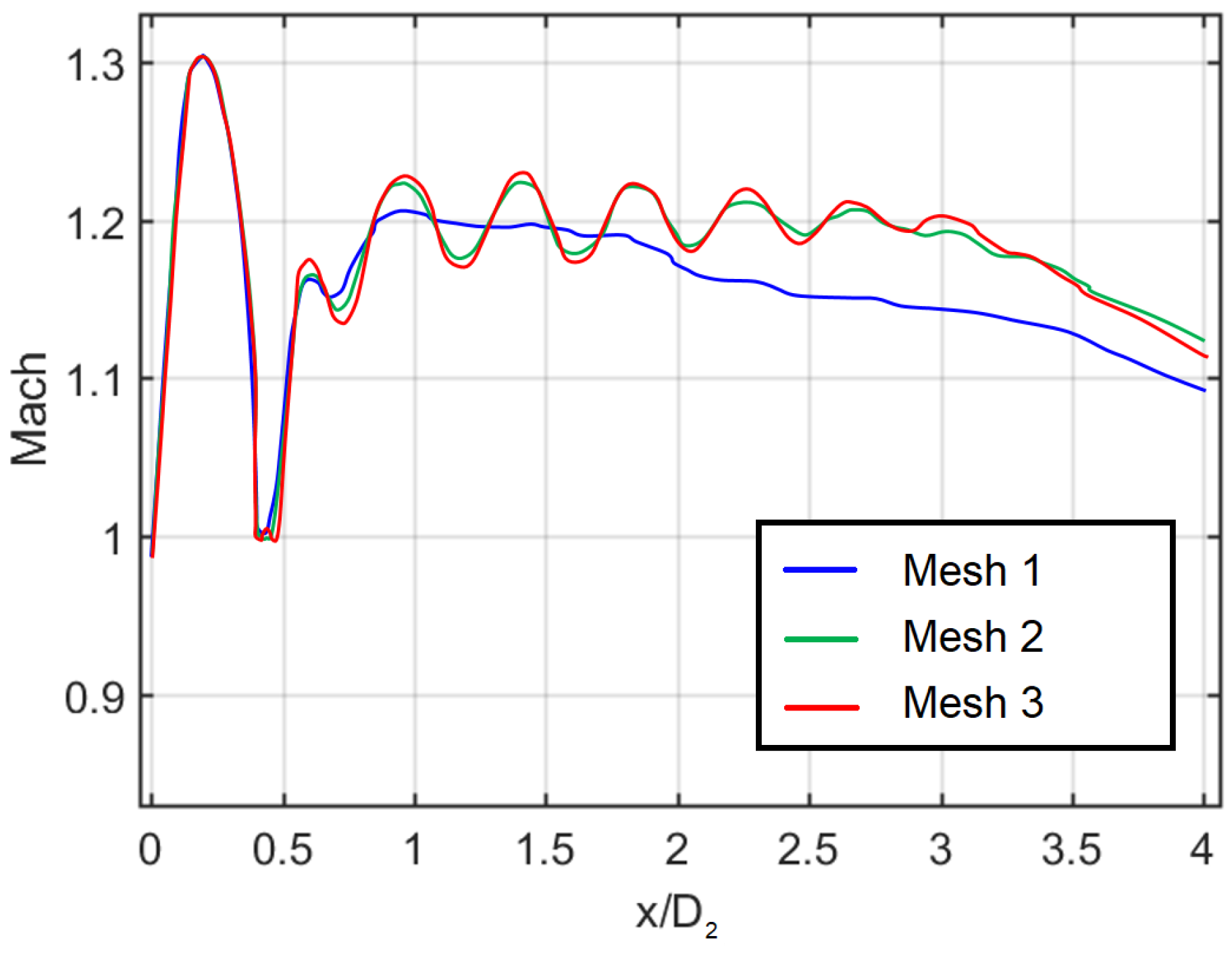
Figure 13.
Results of RANS simulations of the coaxial jet. Axis units are non-dimensionalized by . (a) The velocity field and (b) the pressure field at Condition 01. Mach contour lines in white are superimposed. Data extraction is performed along the dashed black line. (c) The pressure field in Condition 07. Mach contour lines in black are superimposed.

Figure 14.
Pressure field in Condition 08. Mach contour lines in black are superimposed.
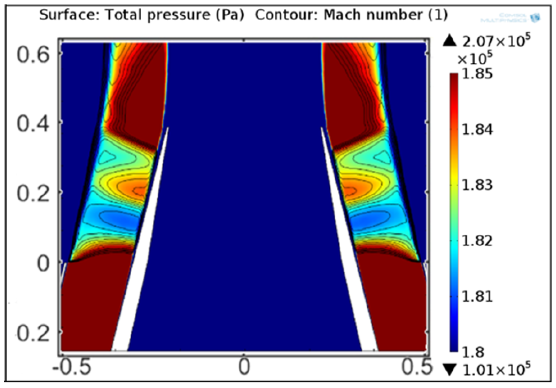
Figure 15.
Sketch and picture of the experimental setup. The laser equipment, source of unwanted noise is located outside the anechoic room. Two spherical lenses and one cylindrical lens have been used to create the laser sheet.
Figure 15.
Sketch and picture of the experimental setup. The laser equipment, source of unwanted noise is located outside the anechoic room. Two spherical lenses and one cylindrical lens have been used to create the laser sheet.
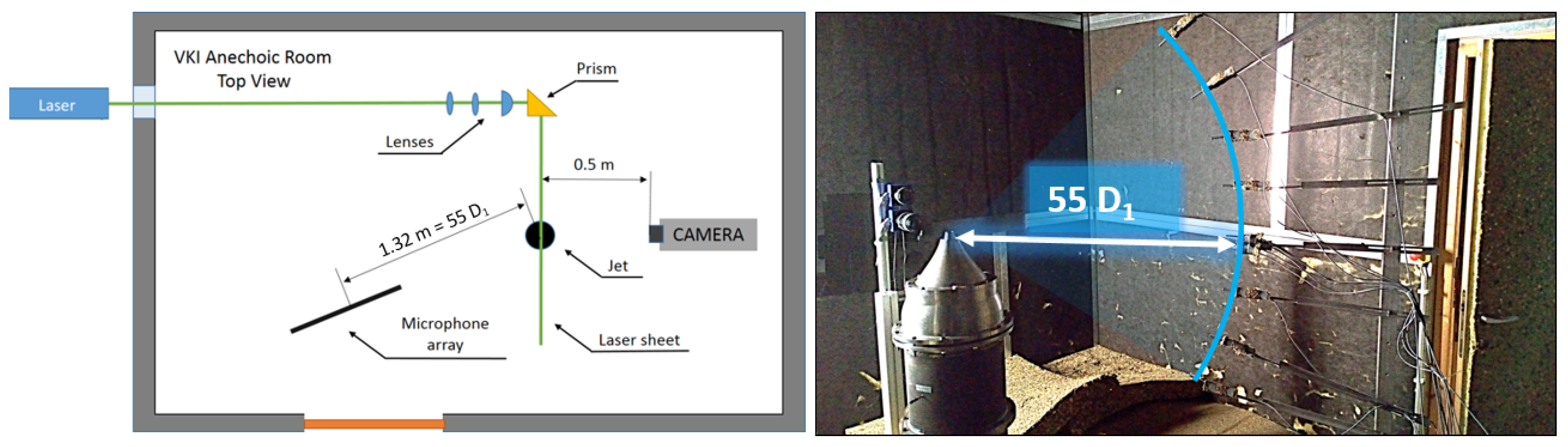
Figure 16.
(a) Example of instantaneous combined FOVs and (b) instantaneous velocity field post-processed using a 12 × 12 pixels final window with 75% overlap for CNPR = 2.50. The flow field shows a system of five shock-cells in line, with the sixth and the seventh one oscillating in antisymmetric motion.
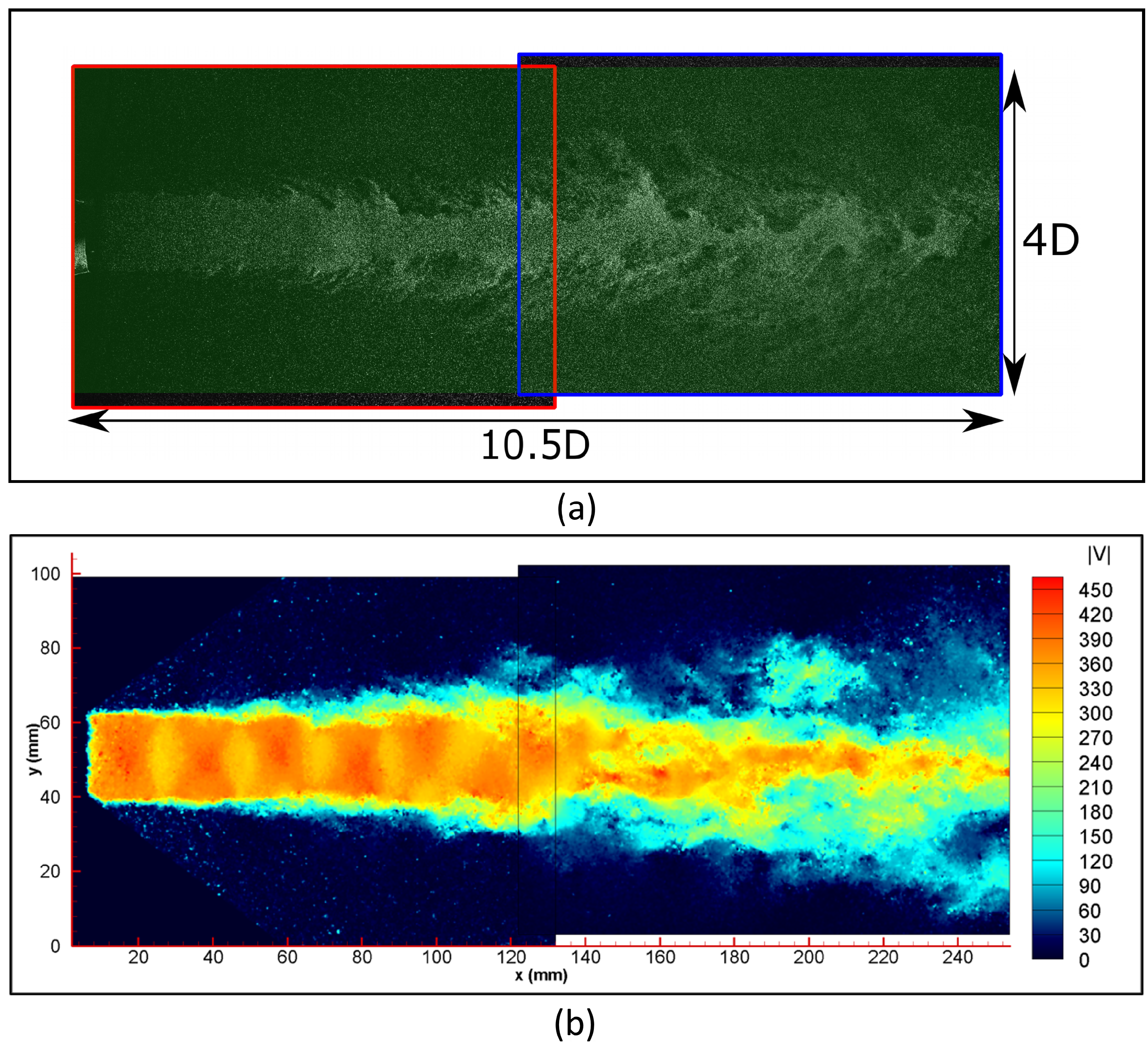
Figure 17.
Overview of the averaged velocity field for all the conditions investigated. Black isocontour lines identify M = [0.9 1.0 1.1].
Figure 17.
Overview of the averaged velocity field for all the conditions investigated. Black isocontour lines identify M = [0.9 1.0 1.1].
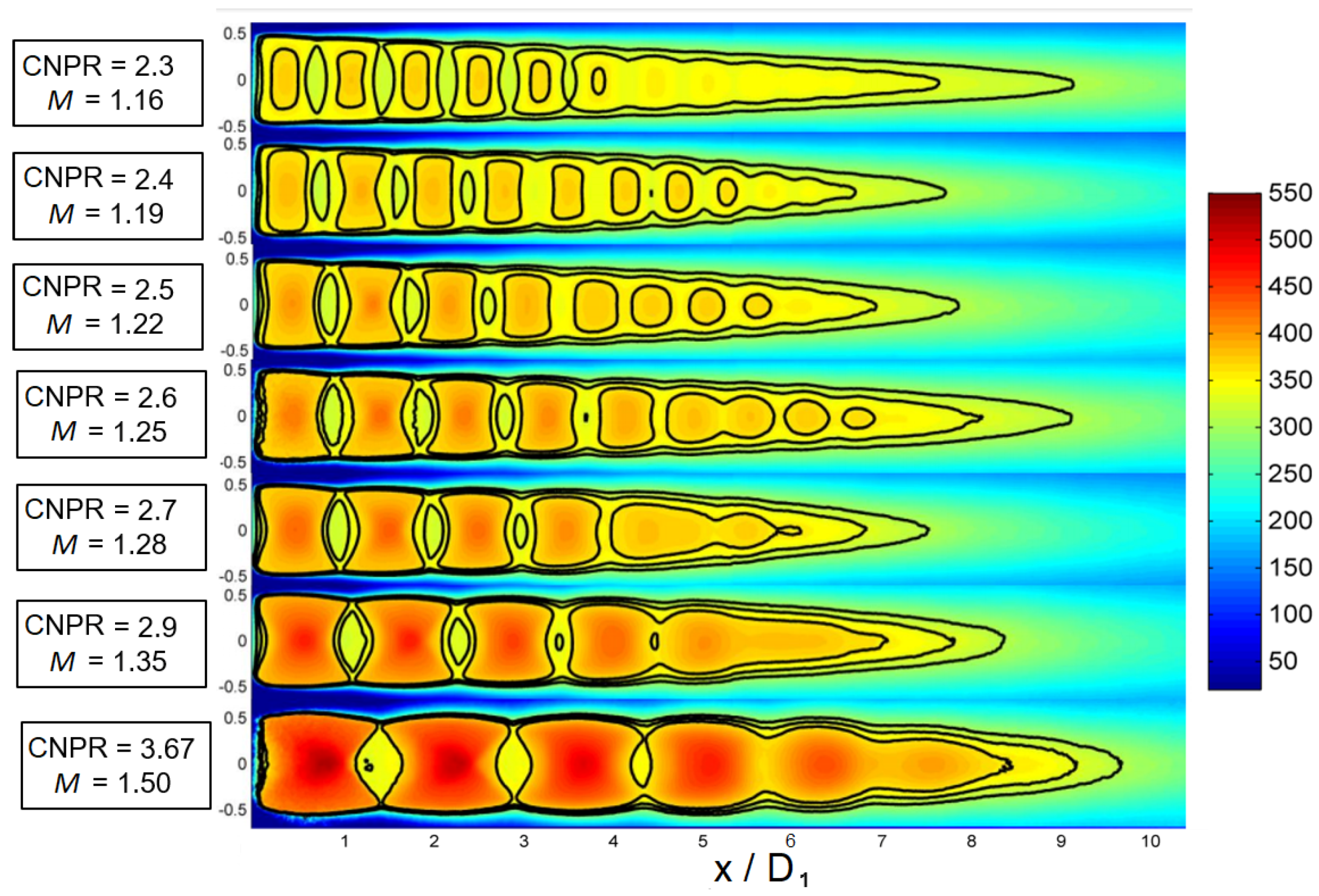
Figure 18.
Mach number profiles in the center line of the jet. Horizontal lines mark the value of the fully-expanded Mach number for each case.
Figure 18.
Mach number profiles in the center line of the jet. Horizontal lines mark the value of the fully-expanded Mach number for each case.

Figure 19.
Normalization of the Mach number profiles in the center line of the jet proposed by Savarese [37].
Figure 19.
Normalization of the Mach number profiles in the center line of the jet proposed by Savarese [37].

Figure 20.
Evolution of the mean shock-cell length with the off-design factor . The black solid line denotes the semiempirical correlation proposed by Harper Bourne and Fisher [38].
Figure 20.
Evolution of the mean shock-cell length with the off-design factor . The black solid line denotes the semiempirical correlation proposed by Harper Bourne and Fisher [38].

Figure 21.
SPL (reference 2 × Pa) at for CNPR = 2.00 (top left), CNPR = 2.26 (top right), CNPR = 2.30 (bottom left) and CNPR = 3.67 (bottom right) at all the measured angles, nozzle diameter m. The images show the switching between two screech modes, from the axisymmetric (top left) to the flapping mode (top right). Many harmonics of the screech tones are visible, and for CNPR = 2.26 also three subharmonics are present. Increasing the Mach number the screech mode switch completely to the flapping mode (bottom left), and then to the helical mode (bottom right).
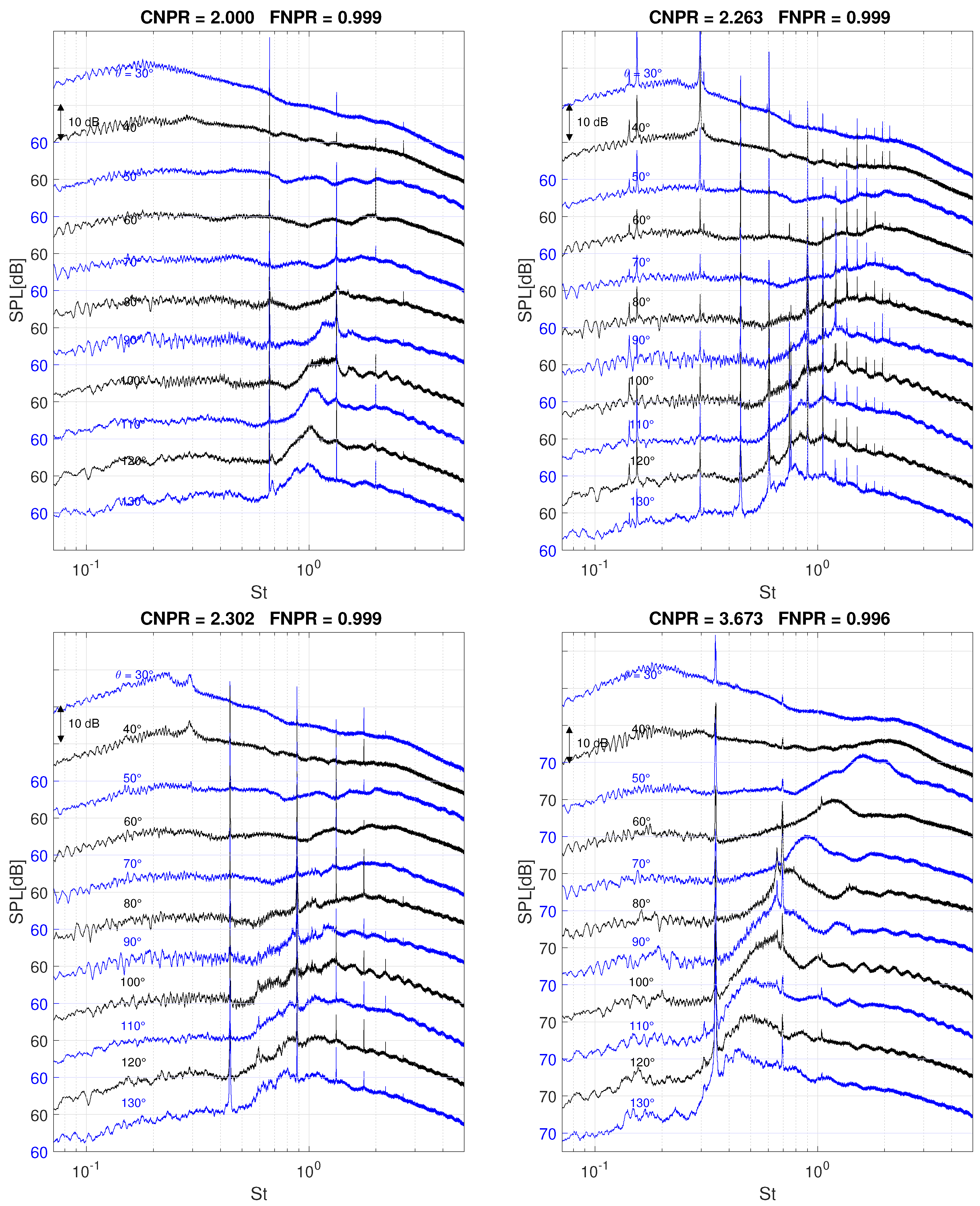
Figure 22.
Variation of the sound intensity with the off-design parameter. The solid line indicates the β4 trend. (a) Microphone located at θ = 30°; (b) Microphone located at θ = 90°.
Figure 22.
Variation of the sound intensity with the off-design parameter. The solid line indicates the β4 trend. (a) Microphone located at θ = 30°; (b) Microphone located at θ = 90°.

Figure 23.
Screech frequency analysis from the results obtained with Nozzle 1. (a) Comparative of measured data with data gathered by Raman [41]; (b) Comparative with screech frequency prediction by Ahuja [39]. Green squares represent the PIV test campaign, while blue dots the acoustic test campaign.

Figure 24.
SPL (reference 2 × Pa) at for several CNPRs at all the measured angles. The red and blue lines are for nozzle diameter m and m, respectively. The drop of the SPL at higher St for the smaller nozzle is due to the limit of the microphones’ dynamic range (70 kHz).
Figure 24.
SPL (reference 2 × Pa) at for several CNPRs at all the measured angles. The red and blue lines are for nozzle diameter m and m, respectively. The drop of the SPL at higher St for the smaller nozzle is due to the limit of the microphones’ dynamic range (70 kHz).
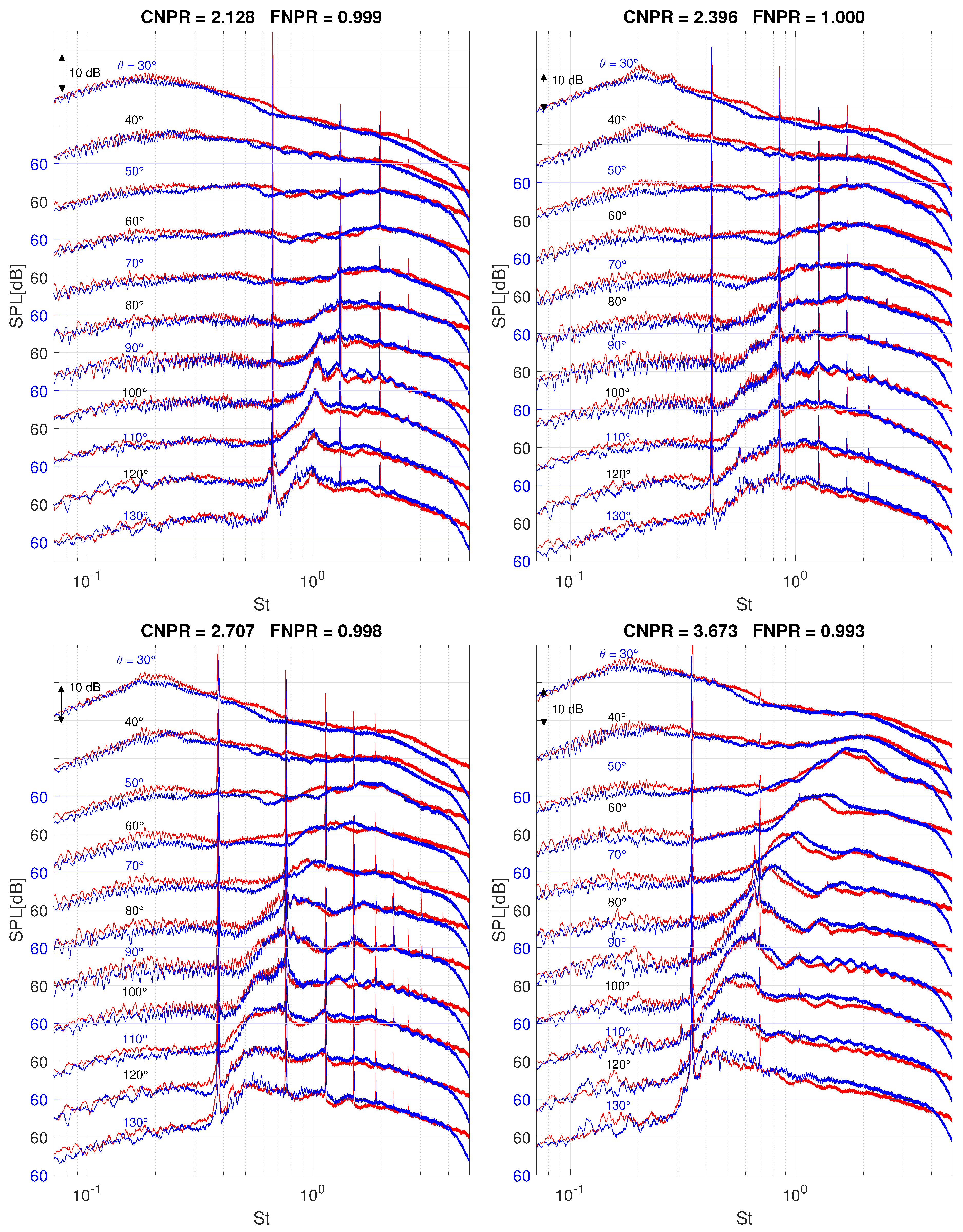
Figure 25.
SPL (reference 2 × Pa) at for CNPR = 2.30 (left), CNPR = 2.36 (right), at all the measured angles; nozzle diameter m. For Nozzle Set 2, the switching from the axisymmetric mode to the flapping mode occurs at higher CNPR compared to Nozzle Set 1.
Figure 25.
SPL (reference 2 × Pa) at for CNPR = 2.30 (left), CNPR = 2.36 (right), at all the measured angles; nozzle diameter m. For Nozzle Set 2, the switching from the axisymmetric mode to the flapping mode occurs at higher CNPR compared to Nozzle Set 1.

Figure 26.
Sketch of the fields of view investigated with PIV. The two green frames on the left are not correlated with the two on the right. The regions enclosed in the red frames, as for the single jet, have been investigated with higher resolution.
Figure 26.
Sketch of the fields of view investigated with PIV. The two green frames on the left are not correlated with the two on the right. The regions enclosed in the red frames, as for the single jet, have been investigated with higher resolution.

Figure 27.
Instantaneous velocity flow field with Mach number isolines for Condition 1. The jet appears to maintain its structure for several jet diameters without losing coherence. The inner jet velocity is modulated by the external flow, eventually reaching sonic speed.
Figure 27.
Instantaneous velocity flow field with Mach number isolines for Condition 1. The jet appears to maintain its structure for several jet diameters without losing coherence. The inner jet velocity is modulated by the external flow, eventually reaching sonic speed.

Figure 28.
Averaged velocity fields with Mach isolines. Based on the radial velocity profiles, the white dashed line is the estimated jet axis. A strong, oblique, shock-wave is present at the end of the primary lip, as expected from simulations. The shock-wave is refracted by the shear layer as a series of expansion waves, which lead then to the formation of the shock-cell system. The shock-cells surround the primary flow and exhibit a regular pattern until the eighth shock-cell. The primary flow velocity is modulated in space following the shock-cells pattern. Some asymmetry is visually perceivable, although a more quantitative approach is requested in order to understand the influence on the flow topology and on the jet noise.
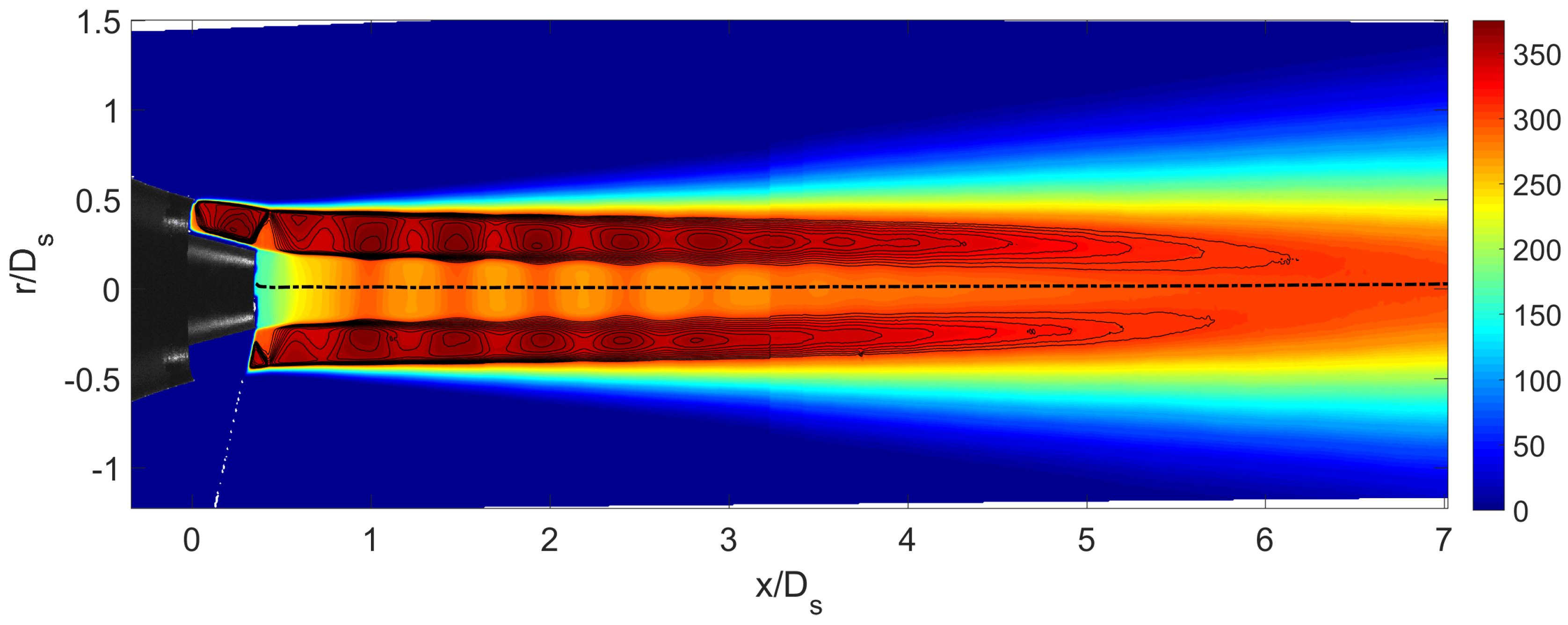
Figure 29.
SPL (reference Pa) at for FNPR = 2.450 and CNPR = 1.675 at all the measured angles, nozzle diameter m and m.
Figure 29.
SPL (reference Pa) at for FNPR = 2.450 and CNPR = 1.675 at all the measured angles, nozzle diameter m and m.


Table 1.
Silencer main dimensions and physical quantities used in the acoustic simulations. and are the main diameter and height, respectively; is the weight; is the max operative pressure; and are the clean passage area and the equivalent diameter for the primary circuit; and are the clean passage area and the equivalent diameter for the secondary circuit. For Grade #000 fine steel wool, is the mean fiber diameter, and is the material apparent density. For the metal canisters, is the area porosity (the hole’s fraction of the boundary surface area); is the plate thickness; is the hole diameter; is the end correction to the reactance; and is the flow resistance.
| 0.98 m | 2.39 × 10 m | 35 m | 0.4 | ||||
| 0.76 m | 2.90 × 10 m | 166 kg/m | 0.25 | ||||
| ∼1200 kg | 0.192 m | 1.5 mm | 0 | ||||
| 11 bar | 0.174 m | 4 mm |
Table 2.
The pressure parameters of the simulation campaign with the relative fully-expanded Mach number, for several test conditions.
Table 2.
The pressure parameters of the simulation campaign with the relative fully-expanded Mach number, for several test conditions.
| Condition | FNPR | CNPR | ||
|---|---|---|---|---|
| 01 | 2.450 | 1.675 | 1.21 | 0.89 |
| 02 | 2.500 | 1.720 | 1.22 | 0.91 |
| 03 | 2.425 | 1.645 | 1.20 | 0.87 |
| 04 | 2.400 | 1.626 | 1.19 | 0.86 |
| 05 | 2.350 | 1.589 | 1.18 | 0.84 |
| 06 | 2.250 | 1.518 | 1.14 | 0.80 |
| 07 | 2.150 | 1.450 | 1.11 | 0.75 |
| 08 | 2.050 | 1.385 | 1.07 | 0.70 |
| 09 | 2.000 | 1.353 | 1.05 | 0.67 |
Table 3.
Meshes main characteristics.
| Maximum Element Size in the Shock Region (m) | Total Number of Elements | |
|---|---|---|
| Mesh 1 | 0.002 | 3.4 × |
| Mesh 2 | 0.0005 | 2.7 × |
| Mesh 3 | 0.00025 | 6.0 × |
Table 4.
Overview of the test conditions investigated during the three campaign carried out using PIV and microphones. Nozzle Set 1 has m, while Nozzle Set 2 has m.
Table 4.
Overview of the test conditions investigated during the three campaign carried out using PIV and microphones. Nozzle Set 1 has m, while Nozzle Set 2 has m.
| CNPR | PIV & Nozzles 1 | Nozzles 1 | Nozzles 2 | (s) | |
|---|---|---|---|---|---|
| 1.8 | 0.96 | x | |||
| 1.9 | 1.0 | x | x | ||
| 2 | 1.05 | x | x | ||
| 2.13 | 1.1 | x | x | ||
| 2.26 | 1.15 | x | |||
| 2.30 | 1.16 | x | x | x | 1.5 |
| 2.36 | 1.18 | x | x | ||
| 2.40 | 1.19 | x | x | x | 1.5 |
| 2.46 | 1.21 | x | |||
| 2.50 | 1.22 | x | x | x | 1.2 |
| 2.60 | 1.25 | x | x | x | 1.2 |
| 2.70 | 1.28 | x | x | x | 1.2 |
| 2.96 | 1.35 | x | x | x | 1.2 |
| 3.67 | 1.50 | x | x | x | 1.0 |
| 4 | 1.56 | x |
© 2018 by the authors. Licensee MDPI, Basel, Switzerland. This article is an open access article distributed under the terms and conditions of the Creative Commons Attribution (CC BY) license (http://creativecommons.org/licenses/by/4.0/).
Share and Cite
MDPI and ACS Style
Guariglia, D.; Rubio Carpio, A.; Schram, C. Design of a Facility for Studying Shock-Cell Noise on Single and Coaxial Jets. Aerospace 2018, 5, 25. https://doi.org/10.3390/aerospace5010025
AMA Style
Guariglia D, Rubio Carpio A, Schram C. Design of a Facility for Studying Shock-Cell Noise on Single and Coaxial Jets. Aerospace. 2018; 5(1):25. https://doi.org/10.3390/aerospace5010025
Chicago/Turabian StyleGuariglia, Daniel, Alejandro Rubio Carpio, and Christophe Schram. 2018. "Design of a Facility for Studying Shock-Cell Noise on Single and Coaxial Jets" Aerospace 5, no. 1: 25. https://doi.org/10.3390/aerospace5010025
Note that from the first issue of 2016, this journal uses article numbers instead of page numbers. See further details here.