Transducer Placement Option of Lamb Wave SHM System for Hotspot Damage Monitoring


1
Aerospace Non-Destructive Testing Laboratory, Faculty of Aerospace Engineering, Delft University of Technology, 2628 CD Delft, The Netherlands
2
Chair of Structural Integrity and Composites, Faculty of Aerospace Engineering, Delft University of Technology, 2628 CD Delft, The Netherlands
*
Author to whom correspondence should be addressed.
Aerospace 2018, 5(2), 39; https://doi.org/10.3390/aerospace5020039
Submission received: 27 February 2018
/
Revised: 24 March 2018
/
Accepted: 28 March 2018
/
Published: 4 April 2018
(This article belongs to the Special Issue Selected Papers from IWSHM 2017)
Abstract
:In this paper, we investigated transducer placement strategies for detecting cracks in primary aircraft structures using ultrasonic Structural Health Monitoring (SHM). The approach developed is for an expected damage location based on fracture mechanics, for example fatigue crack growth in a high stress location. To assess the performance of the developed approach, finite-element (FE) modelling of a damage-tolerant aluminum fuselage has been performed by introducing an artificial crack at a rivet hole into the structural FE model and assessing its influence on the Lamb wave propagation, compared to a baseline measurement simulation. The efficient practical sensor position was determined from the largest change in area that is covered by reflected and missing wave scatter using an additive color model. Blob detection algorithms were employed to determine the boundaries of this area and to calculate the blob centroid. To demonstrate that the technique can be generalized, the results from different crack lengths and from tilted crack are also presented.
1. Introduction
Non-Destructive Testing (NDT) [1] has been implemented in many industries to ensure structural safety and reliability. Structural Health Monitoring (SHM) as a complementary solution with respect to the already existing NDT techniques has been a subject of interest in the past decade due to its potential economic benefit, particularly in structural maintenance [2,3].
Along with fiber-optic techniques such as Fiber-Bragg-Grating sensors [4,5], an ultrasonic guided waves-based solution such as those making use of Lamb waves is one of the promising techniques for SHM due to its long-range inspection capability up to several meters [6,7], which is suitable for monitoring large structures such as an aircraft fuselage. Also, in comparison to the FBG technique, Lamb wave SHM sensors typically require less complicated installations. This is particularly useful for monitoring aircraft which are already in-service, since aircraft operators generally tend to be reluctant to make larger modifications.
Lamb wave damage monitoring relies on the detection of interactions between the Lamb wave and the damage [8]. Various properties of propagating wave are modified by the crack and various properties of the signal such as amplitude, frequency, phase, etc. are assessed to calculate the damage index (DI). The most commonly used sensors for generating and capturing Lamb waves are piezoelectric transducers (PZT) [9]. Since PZTs are permanently attached to the surface of the structure, sensor placement becomes tremendously important because the quantification of DI relies heavily on the sensor positions. A poor transducer placement will result in weak or undetected capture of wave scatter which in turn decreases the damage detectability of the SHM system.
The literature describes different approaches for sensor placement options, such as prioritizing the sensor location based on a detectability limit [10], using a modal analysis parameter determination for damage localization assessment on a truss structure [11], and by using global search and greedy algorithms [12]. Li et al. [13] proposed a sensor optimization algorithm based on maximum energy consumption on sensor candidate location of a civil engineering structure.
Fendzi et al. [14] proposed a novel approach for sensor placement by using geometric dilution of precision (GDOP), which is based on Lamb wave ray tracing method for known damage locations. Haynes [15] proposed sensor placement by minimizing the Bayesian cost to select locally optimal sensor locations. However, if the damage occurs outside of the designated area, the system might fail to detect it. A similar approach by using Bayesian experimental design has been conducted by Flynn and Todd [16].
Furthermore, Sun et al. [17] performed discrete optimization by using the artificial bee colony algorithm to optimize their objective function which is based on modal assurance criterion (MAC). Similar approaches by using search metaheuristics were also delivered by Yi et al. [18], Zhao et al. [19], and Shan et al. [20]. In more recent study, Capellari et al. [21] proposed an optimal sensor placement by employing Polynomial Chaos Expansion and stochastic optimization to maximize the gain in Shannon information.
Thiene et al. [22] introduced the DI-free sensor placement optimization based on the fitness function which maximizes the coverage area of the sensor network. They calculated the coverage of each pixel in the geometry based on pitch-catch technique, so that every pixel that contributes to the probability that a damage in random location is being detected is counted. Venkat et al. [23] used a Finite Element (FE) simulation platform to build differential images between the undamaged and damaged structure. They plotted the summed-up energy captured by all sensors and determined the most optimal sensor location by the highest captured energy.
From all these studies, we concluded that most of the sensor placement strategies are for civil engineering structures and that one of the most common features used for the objective function is the MAC, which is typically applicable for low-frequency vibrations. However, we have not seen any application using MAC in Lamb wave SHM frequency, which is normally above 100 kHz. Only [14,15,16,22,23] are related to sensor placement for guided wave SHM.
Summarizing references [14,15,16,22,23], there are two streams of sensor placement research that are specialized for guided wave-based SHM: (1) The approach exhibiting known area of damage location; and (2) The random damage location approach. If a damage location can already be approximated by analytical methods from fracture mechanics, FE simulation and fatigue testing, then the optimum sensor location can be determined by maximizing the DI of the sensor network around the predicted damage location. However, for random location damage such as hail impact, a different objective is needed.
From this current state of the art, our work is performed to develop the work presented in two most recent articles [22,23]. For this paper, the objective is to propose an image processing for known damage location approach, known as hotspot SHM [22].
Due to the expected number of different damage locations occurring in an aircraft fuselage multiplied by the numerous possibilities for sensor placement, conducting an experiment or even a numerical simulation to track the wave scatter is not practical. To address this issue, we propose a design for a sensor placement in a hotspot SHM system based on an additive color model and blob detection algorithm that can detect residual wave scatter from simulation data.
After the introduction in Section 1, we have structured the paper as follows: In Section 2, we briefly review the Lamb wave propagation theory whose effect is employed in Section 3 for determining the SHM sensor positions by using image processing for predictable critical crack size, location, and orientation. The results and concluding remark are presented in Section 4 and Section 5, respectively.
2. Lamb Wave Propagation
First described by English mathematician Horace Lamb in 1917 [24], the description of acoustic wave propagation in solid plates has been evolving ever since. A theoretical analysis of Lamb wave propagation in metallic materials, composite, and hybrid materials is described in [25,26,27]. The elastodynamic wave equation for an anisotropic inhomogeneous medium in a d-dimensional bounded domain Ω ⊂ ℝd (d = 2, 3) is given in by:
where u(x,t) is the time and space dependent displacement, ρ the material density, Cijkl the material stiffness tensor, εkl the strain tensor, and f(x,t) the source function, respectively. After applying boundary conditions of two parallel surfaces, there are two solutions to Equation (1) for wave propagation in homogeneous material of given density, described by:
which are well-known as symmetrical (S-Mode) and anti-symmetrical (A-Mode) Lamb wave propagation modes, respectively. The definitions of p and q are given by:
where ω is the frequency, cL is the longitudinal bulk wave velocity, cT is the transversal bulk wave velocity, and k is the wavenumber. The numerical solution of Equations (2) and (3) can be drawn as a dispersion curve, which describes the wave velocity as a function of frequency-thickness product [28].
As they introduce potentially overlapping signals, higher-order Lamb modes are generally undesirable, and the maximum cutoff frequency is normally determined as before the A1 mode appears.
3. Sensor Positioning Approach for Hotspot SHM
This section describes the developed methodology for sensor placement in hotspot SHM. It considers: (1) Crack growth and critical crack size in a damage-tolerant aircraft substructure; (2) Numerical simulation of Lamb wave propagation in a plate-like structure; and (3) Image processing that involves displacement subtraction of damaged from undamaged structures.
3.1. Crack Growth in Damage Tolerance Structure
To understand deterministic sensor positioning for a predictable crack location, firstly, it is important to understand the concept of damage-tolerant design. The definition of damage tolerance is “the ability of the structure to sustain design limit loads in the presence of damage caused by fatigue, corrosion and other sources until such damage is detected and repaired” [29]. The important key elements in damage tolerance design are: (1) the assumption of initial damage existence; (2) damage growth in the material due to structural loading; and (3) The critical damage size up to which the structure endures the loading before catastrophic failure. These three key elements are synchronous to the regions I, II, and III in a typical da/dN curve [30], which describes crack propagation rate as a function of stress intensity factor (SIF) range during fatigue cycling (ΔK).
The assumption of initial crack existence falls in region I, where the crack growth is typically slow. This region can be covered by some advanced (but also large and expensive) NDT and material characterization techniques such as X-ray computer tomography [31] or scanning electron microscopy (SEM) [32]. After passing the threshold stress intensity factor range ΔKth, region II begins where the crack propagation rate is stable, and crack growth normally follows the Paris-Erdogan law [30,33], which has Paris-Erdogan constants C and m. In this region, the crack becomes much larger and sometimes can be seen with naked eye [34]. After transition between region II and III, the crack propagation rate becomes rapid and unstable until final failure.
Lamb waves can interact with a crack which has a size at least the half of its wavelength [35,36], and since the critical crack tolerant size (which can be up to several hundred millimeters [22]) is generally larger than the wavelength (which is typically less than 100 mm), it is safe to assume that Lamb waves can also interact with the critical crack. Fracture mechanics and fatigue analysis can predict the most probable crack location for certain loading conditions [37].
The SIF is generally larger in the area around the notch, thus one can expect that a crack will occur around a notch. For example, the changes in cabin pressure in an aircraft fuselage can be approximated by the internal pressure in a thin-walled cylinder where the hoop stress is two times larger than the axial stress [38]. Therefore, the crack orientation is expected to be orthogonal to the direction of the hoop stress. By knowing the most probable crack orientation and location and the critical crack size for a certain geometry, two FE simulations scenarios of wave propagation can be performed [39]: (1) Lamb wave propagation in an undamaged structure as a baseline and (2) Lamb wave propagation in a critically damaged structure.
3.2. Simulation of Lamb Wave Propagation
The FE formulation for Lamb wave propagation is based on Hamilton’s principle [40] as described in:
where Γ and Φ are the surficial and volumetric integral areas, ρ is the material density, u and ü are the particle displacement vectors in the material and their corresponding accelerations, respectively, ε is the strain tensor and Cijkl is the stiffness matrix. The external forces can be classified as surface load FS and volume load FV. To numerically solve Equation (6), the geometry involved is divided into discrete mesh elements over which the equation can be approximated [41]. For a 3D-problem, there are four element types: prism, pyramid, brick and tetrahedron [42]. To reliably model an ultrasonic signal, the recommended number of mesh elements is 4 elements per A0- or 8 per S0-wavelength [43].
3.3. Additive Color Model
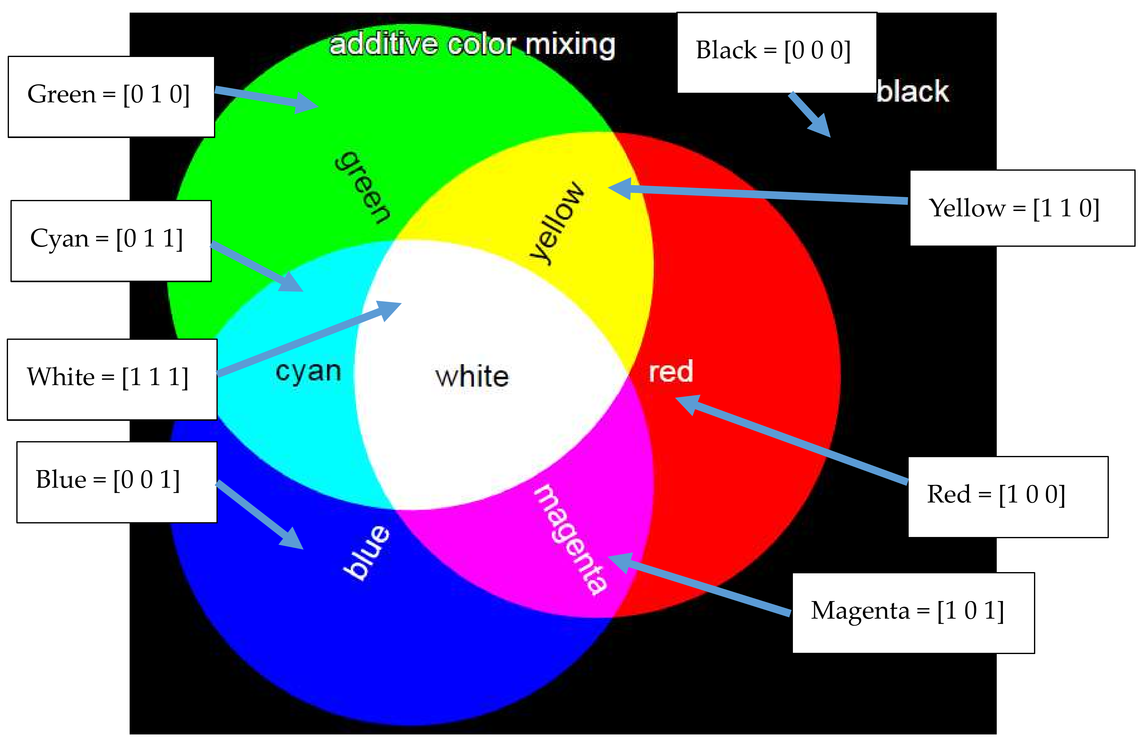
Mathematical representations of color can be summarized as additive and subtractive color models [46]. The additive color model is used for combining light of different color and the subtractive color model is used for combining pigments and dyes, which are typically represented in 4 basis colors: cyan, magenta, yellow, and black (CMYK).
Both additive and subtractive color models are typically represented in vector form. Both color models relate to the perception of the human visual system. In the additive color model, the background is black, and color is composed of a red, green, and blue (RGB) tuple as depicted in Figure 1. This relates to the three cone cells of the human retina (long, medium, and short) which have peak sensitivities to light of wavelengths 559 nm, 531 nm, and 419 nm. These correspond to red, green, and blue light, respectively [46]. Normally, red, green, and blue color may be written in 8-bit form as [255 0 0], [0 255 0], and [0 0 255], respectively or in normalized form as [1 0 0], [0 1 0], and [0 0 1], respectively.
When working with digital imaging, the additive color model (i.e., RGB) is a natural choice because what humans see in a measurement device/computer screen is normally encoded in RGB values. Computer scientist and electrical engineers have selected to represent the digital vision (e.g., in computer monitor) as an RGB array because of the trichromatic cone cells in human eye which are sensitive to the frequency spectrum of red, green, and blue photons that are falling into human retina. Therefore, the origins of the additive color model are physical and biological rather than purely technical.
In the 3-bit model, shown in Figure 1, other colors such as cyan, magenta, yellow, and white are obtained by adding basic colors. For instance, cyan is the addition of blue and green, while white is the addition of red, green, and blue. Colors may also be subtracted from one another, as given in Table 1. Note that in the convention used negative values are set at zero, as negative light amplitude has no physical meaning. In this paper, material displacements are represented as colors in the additive color model and mathematical operations are performed to identify and visualize the optimum sensor positions.
4. Results and Discussion
4.1. Simulation
The method for choosing the simulation parameters has been described in [23,43]. The plate dimensions are 600 mm × 400 mm × 2 mm. For this work, the following parameters are used: ABAQUS explicit, aluminum properties (Young’s modulus of 70 GPa, Poisson ratio of 0.33, density of 2700 kg/m3), quadratic brick mesh (C3D20) with a global mesh size of 1 mm, single node out-of-plane excitation with windowed 5 sine-cycle of central frequency of 250 kHz with 1 N concentrated force, dynamic implicit step, no boundary conditions imposed, time increment of 0.1 μs (which means a sampling frequency of 10 MHz), total time period of 500 μs and a single nodal output precision. The specification of the computer where the simulation was run was: Intel Xeon E5-1620 3.5 GHz (Quad-core 8-Threads), 32 GB DDR3-RAM, and NVidia NVS310M Graphic card (GPU acceleration was not activated).
4.2. Data Extraction
To capture the wave propagation image, the screenshot program which is called Lightshot can be downloaded from prntscr.com [47]. In the program settings, the option “Keep the selected area position” must be selected so that Lightshot remembers the X-Y position of the captured screenshot for every time increment. As mentioned previously, this technique is less exhaustive and more memory efficient as every saved image has a size of only around 500 KB. For 20-time increments and 2 cases (uncracked and cracked plate), only around 20 MB of space is needed in comparison to ODB extraction which takes around 3.2 GB of space.
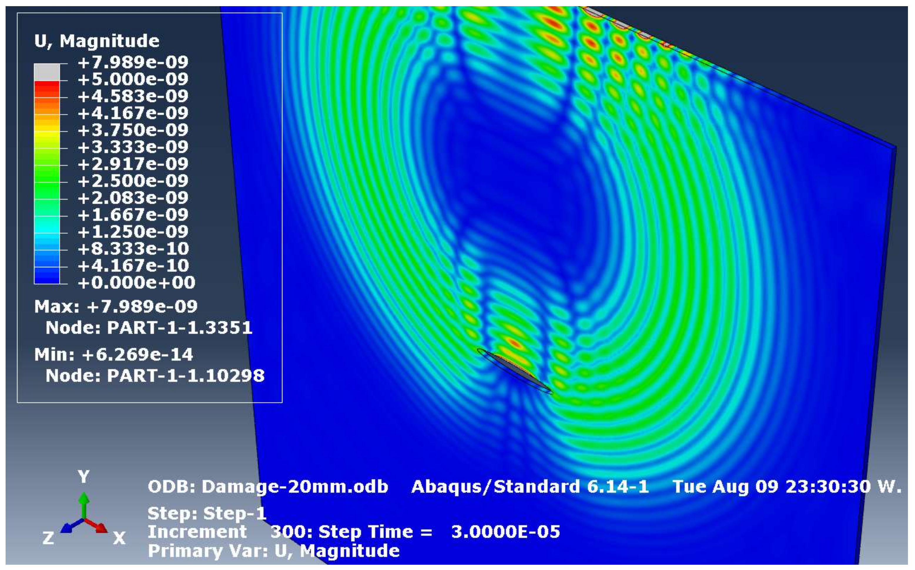
In a computer, the color in a single pixel is represented as an RGB array and this can be used to represent different Lamb wave displacement amplitudes. Figure 2 shows an example simulation of Lamb wave propagation 30 μs after excitation. The displacement magnitude U is defined as:
where Ux, Uy, and Uz are the displacements in the x, y, and z-directions, respectively. It is obvious that no displacement (U = 0 nm) is shown as a blue pixel, while a displacement of 2.5 nm is shown in green, and a displacement of 5 nm is shown in red. The values in-between such as 1.25 nm and 3.75 nm are shown in cyan and yellow, respectively.
This colormap ‘rainbow’ is the default colormap in ABAQUS. Note that this colormap is slightly different from the basic 3-bit RGB colormap depicted in Figure 2 as it has more color transitions, i.e., there are smoother transitions between blue and cyan, cyan, and green, and so on. For ease, we neglected displacements larger than 5 nm (shown in grey color), which are mostly due to the excitation, because in this simulation this only appears in few locations. While this image processing procedure offers less displacement information as all displacement values are translated into an RGB array, we find this alternative procedure much faster, and more memory efficient rather than extracting data directly from the ABAQUS ODB binary file.
4.3. Differential Images
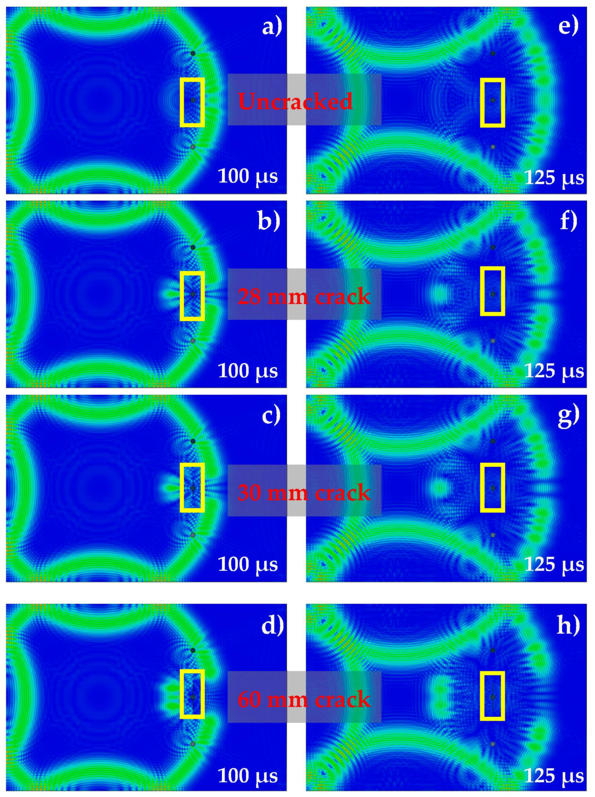
The approach is demonstrated by taking screenshots from the ABAQUS Viewer User Interface. Figure 3a shows Lamb wave propagation at t = 100 μs in an uncracked Al-7075 plate. The simulation images are actually similar to those which are depicted in Figure 4 of [16], except that the simulation platform, color map, excitation signal, and the geometries are slightly different.
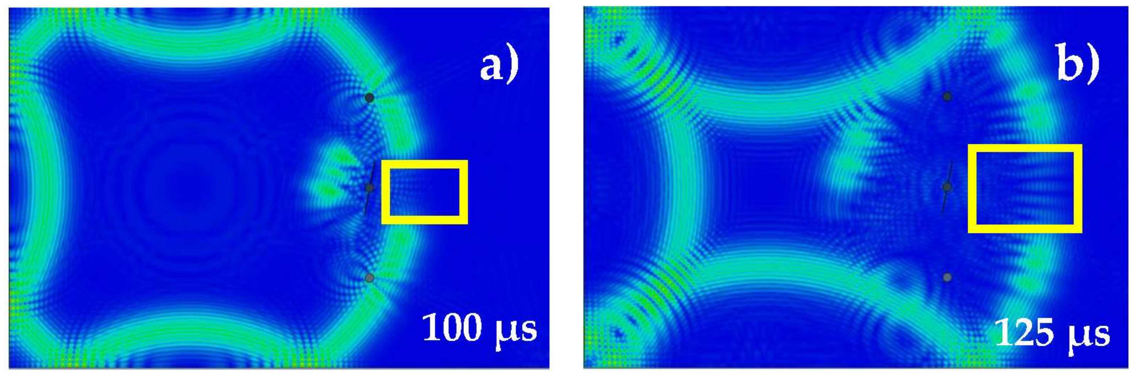
The plate contains 3 rivet holes as depicted in Figure 3a,b shows Lamb wave propagation in the same plate but with a symmetric crack (from tip-to-tip, including the hole diameter of 10 mm) of 28 mm length in the middle of the plate (marked by a yellow rectangle). The images captured have size of 1210 × 807 pixels, so the resolution is 2 pixel/mm. Images are stored as matrices with a size of 1210 × 807 × 3, where each pixel has 3 arrays, each containing a normalized floating value between 0 and 1 for each of the RGB colors.
A similar pattern of Lamb wave propagation can be observed if the crack length differs by +/− 10%, as shown in Figure 3c. In this case, the crack length is 30 mm instead of 28 mm. However, if the crack is much larger, a notable change in the wave propagation pattern can be observed, as depicted in Figure 4d. In this case, the crack length is 60 mm. Similarly, the wave propagation at t = 125 μs for an uncracked plate, and for plates with crack lengths of 28 mm, 30 mm, and 60 mm can be observed in Figure 3e–h, respectively.
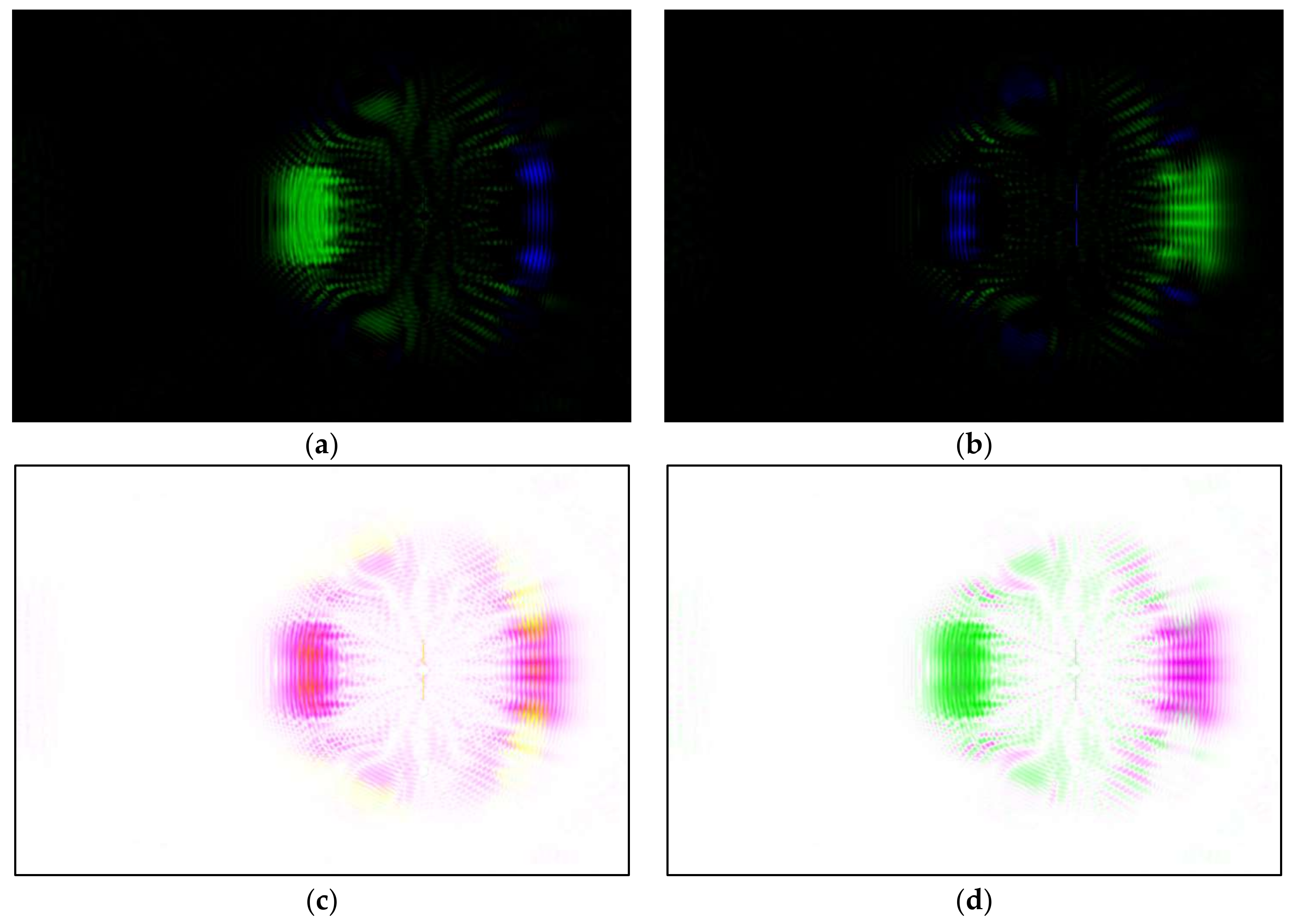
By subtracting the image of the cracked plate (Figure 3h) from that of uncracked plate (Figure 3e), the reflected wave scatter image can be obtained, as shown in Figure 4a. Note the RGB values are subtracted rather than the displacement values. Pixels, for which there is no change in wave scatter are shown as black. In this figure, the reflected wave scatter is highlighted by the yellow rectangle, while the corruptly transmitted wave is obtained as well (in the red rectangle) but is not clearly visible.
In an analogous way, we can subtract Figure 3e from Figure 3h, and in this case, the corruptly transmitted wave scatter image is highlighted more (red rectangle) as depicted in Figure 4b, while the reflected wave scatter can still be seen (yellow rectangle) but is less visible. For the further sections in this paper, only the results from the uncracked plate and the cracked plate of 60 mm crack will be shown for conciseness. To highlight both the reflected and corrupted wave scatter, the two images shown in Figure 4a,b can be joined to form a composite image.
Two common ways combining images are described here, the first one is called image addition. In this case, both image matrices are just mathematically added. The second one is called image fusion and uses the ‘imfusion’ function in MATLAB, where the two images are firstly converted into greyscale mode, given a false color, and then added mathematically. Furthermore, it is possible to invert the composite images to obtain the inverted images. This step is not necessary, but some people subjectively may find the colored wave scatters easier to track if the background is white. The inverted images from image addition and image fusion are depicted in Figure 4c,d, respectively. For the sensor placement procedure described in Section 4.4, the inverse fused image (Figure 4d) is used because we can still see the representation of reflected and missing wave scatter and that enables us to cross check the results with the simulation data.
4.4. Sensor Placement
The wave scatter which was caused by both reflections and corrupted transmissions due to the crack front are represented by false color (i.e., green and magenta pixels in Figure 4d). These pixels have a different color from the background (white). Regions of interest are determined by using the Matlab blob detection function to locate areas of adjacent green and magenta pixels. The larger the blob is, the larger the area of wave scatter. The sensor should be placed in the center of the largest blob, so that it will have a high probability of capturing a portion of wave scatter from cracks.
The blob detection algorithm is based on the Laplacian of Gaussian [48,49,50] with a kernel of 8-pixel connectivity. Given the Gaussian function G of an input image f(x,y) and feature scaling σ as given in Equation (8). The Laplacian operator ∇2 is given in Equation (9).
By applying the Laplacian operator in Equation (9) to the Gaussian function in Equation (8), one obtains the Laplacian of Gaussian, commonly known as LoG, as described in Equation (10). Hence, the blob centroid , with the scale is the simultaneously local extremum of the LoG in Equation (11).
For the blob detection, the kernel of 8-pixel connectivity is used because it is more suitable for a larger area since the diagonal neighbor is counted as well, see Figure 5a, while 4-pixel connectivity (Figure 5b) is typically used for line and corner detection. In Figure 5a,b, the meaning of −1 and 0 are pixels which are counted and are not counted as a neighbor of the center pixel, respectively.
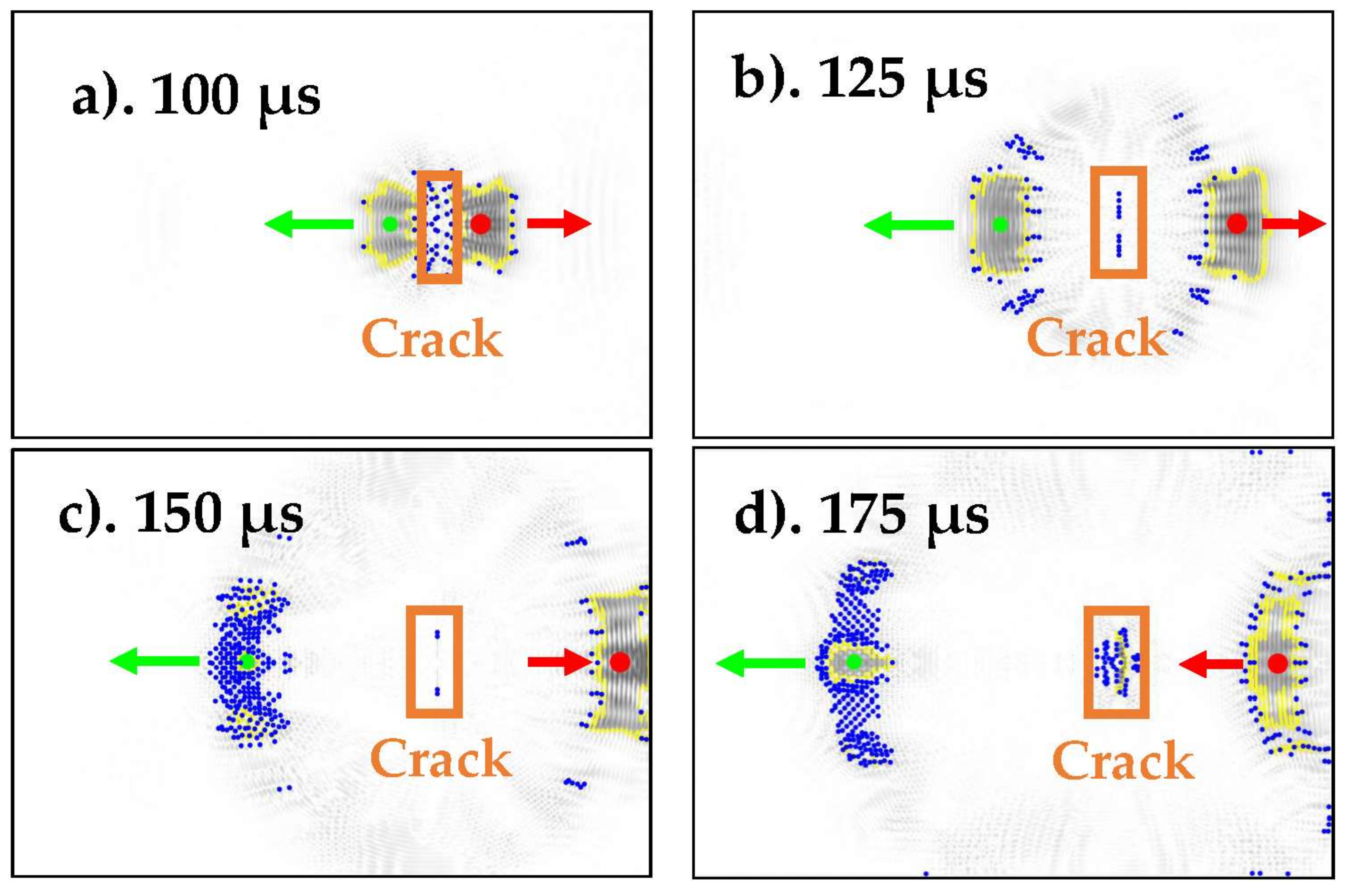
The blob detections from various time increments are depicted in Figure 6a–d. As mentioned before, we would like to place the sensor in the location with the largest change in signal over time, i.e., the largest blob. Since it generally contains more than a single pixel, the centroid can be calculated to determine the average pixel location that would receive wave scatter. In Figure 6a–d, the largest and the second-largest blob centroids are marked by red and green dots, respectively. Blob boundaries are marked by the yellow polylines.
The rest of the centroids are marked by blue dots. In order not lose the overview, the reader is encouraged to compare Figure 6a with Figure 3a,d, as well as Figure 6b with Figure 3e,h. The X-Y coordinates of the blob centroid and the blob size are summarized in Table 2. The detailed procedure in MATLAB to find to trace the blob is described in Algorithm 1.
| Algorithm 1: Algorithm for blob detection and centroids calculation | Meaning: | |
| 1 2 3 4 5 6 7 8 9 10 11 12 13 14 15 16 17 18 19 20 | j ← number of available image files for i ← 1:j img[i] ← imread(image[i]) I[i] ← mat2gray(rgb2gray(img[])) BW[i] ← I[i] < threshold B{i} ← boundaries(BW,8) s(i) ← regionprops(BW end n ← number of detected blobs for m ← 1:n S[m] ← s[m].Area [val ind] ← sort(S,‘descend’) boundary{m} ← B{ind(m)} centroids[m] ← mean(boundary{m}) X ← [X centroids(2)] Y ← [Y centroids(1)] end | Assign j as the number of available images Loop over images from 1 to j: Store the image in matrix ‘img’ Convert the RGB array into greyscale Set the pixel intensity threshold Trace region with 8-pixel connectivity Open the region properties End the loop Assign n as the number of detected blobs Loop over all traced region from 1 to n: Store the area information in matrix ‘S’ Sort from the largest to smallest blob Store the blob boundaries Calculate blob centroids Assign X-coordinate from the centroid Assign Y-coordinate from the centroid End the loop |
After a certain time, the wave pattern becomes more chaotic due to multiple reflections from the crack front, rivet holes, and plate edges so that more smaller centroids will be born that are not exactly aligned with the mid Y-axis anymore. The smaller centroids imply that the potential energy capture by PZT is getting smaller and this will be aggravated by Lamb wave attenuation. This is the reason we recommend ‘early wave scatter capture’ for hotspot SHM design. Typically, one can decide the best sensor position by considering the movement of the centroid per time increment, also known as ray tracing [51].
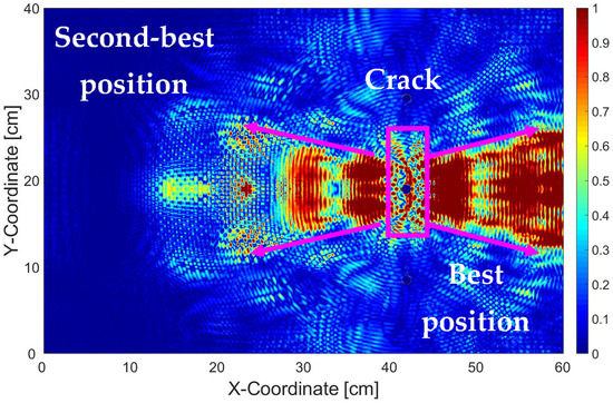
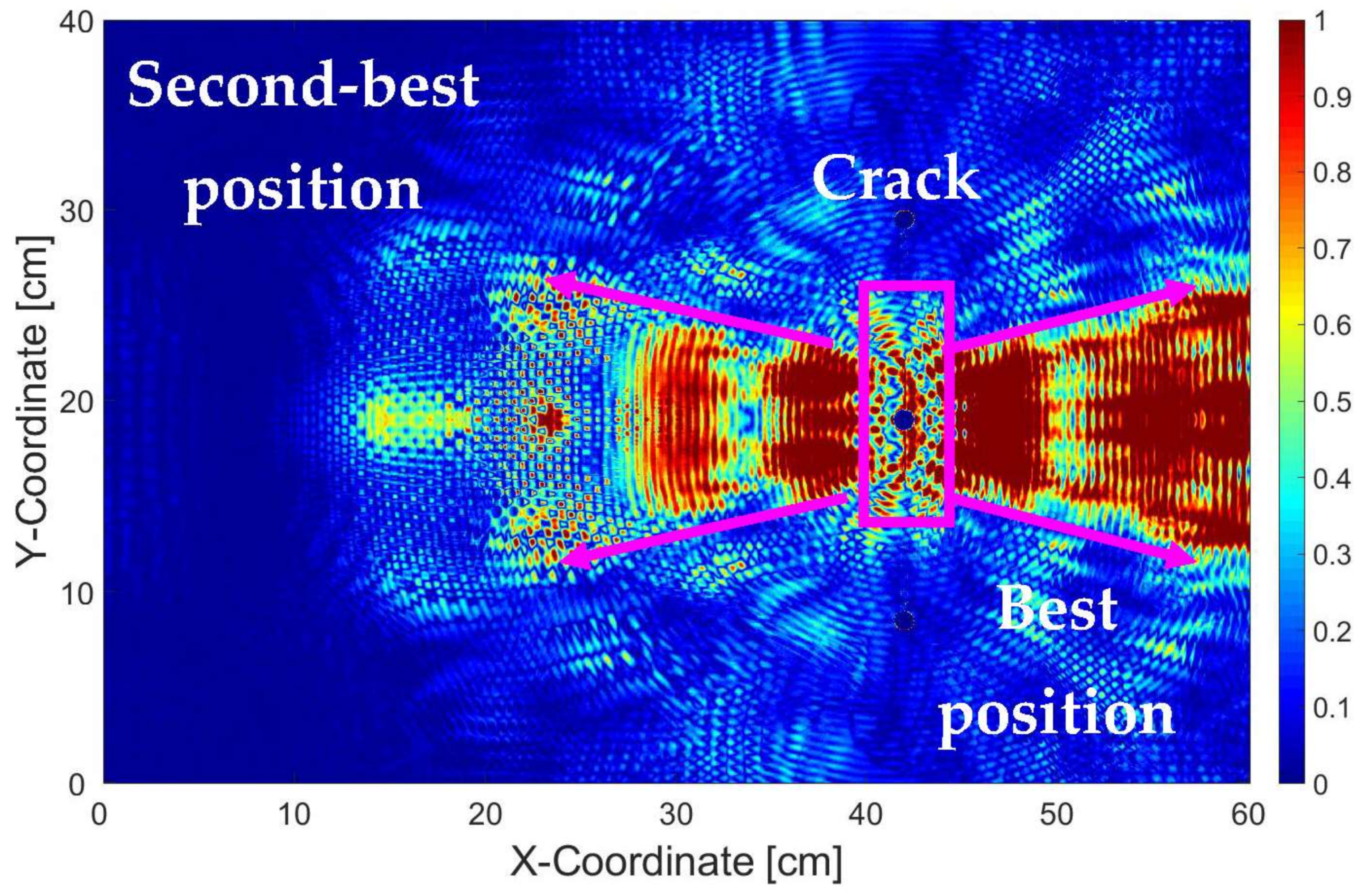
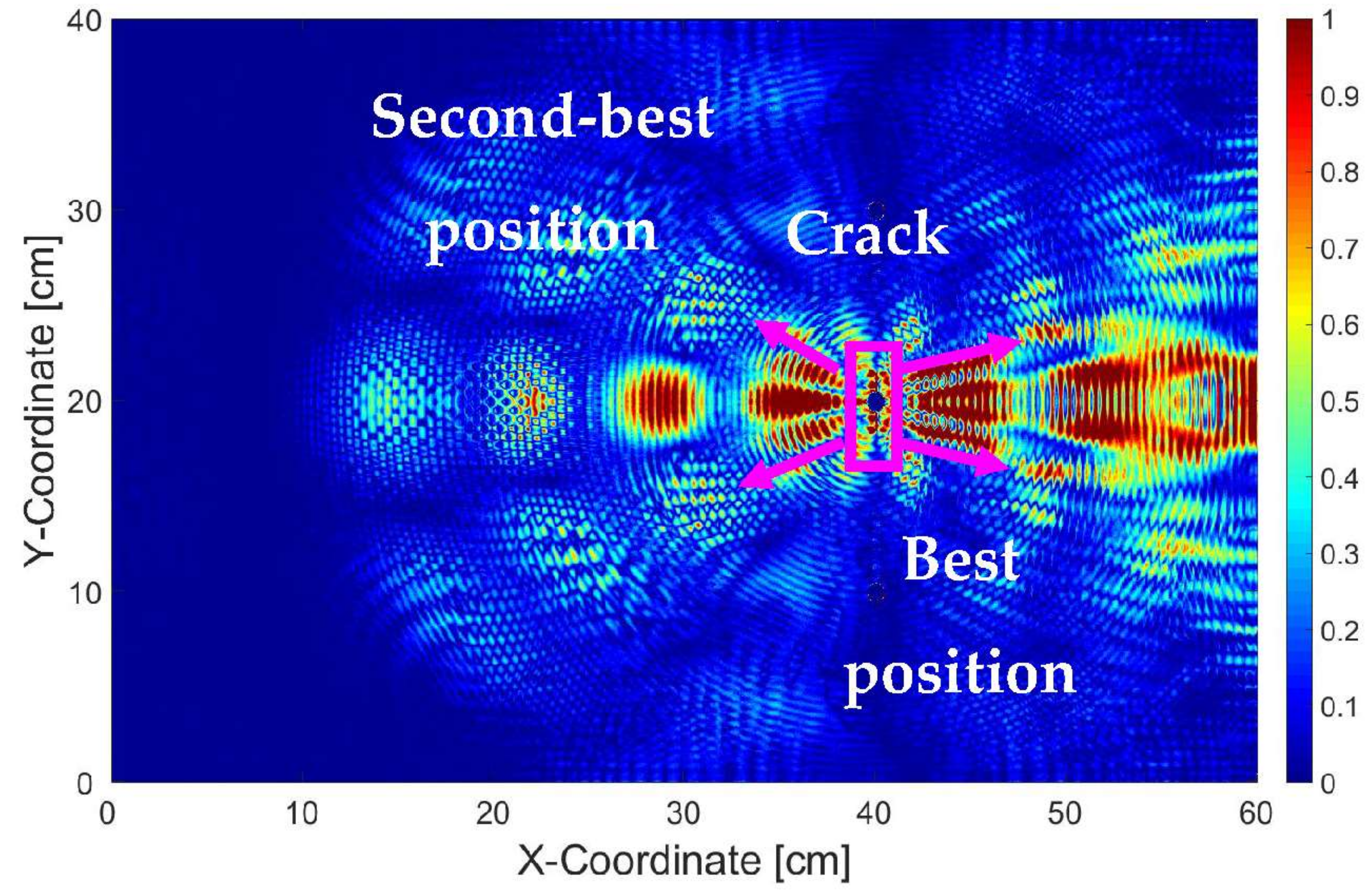
Furthermore, it is possible to fuse Figure 6a–d into a single image. We performed this operation and the result is depicted in Figure 7, where each pixel contains information about the normalized intensity between 0 and 1 which is then mapped into the rainbow color scale. From Figure 7, it can be subjectively judged that the best sensor position is between X = 44 cm and 57 cm and the second-best sensor position is between and X = 34 and 38 cm, while the vertical coordinate for both positions remains at Y = 20 cm.
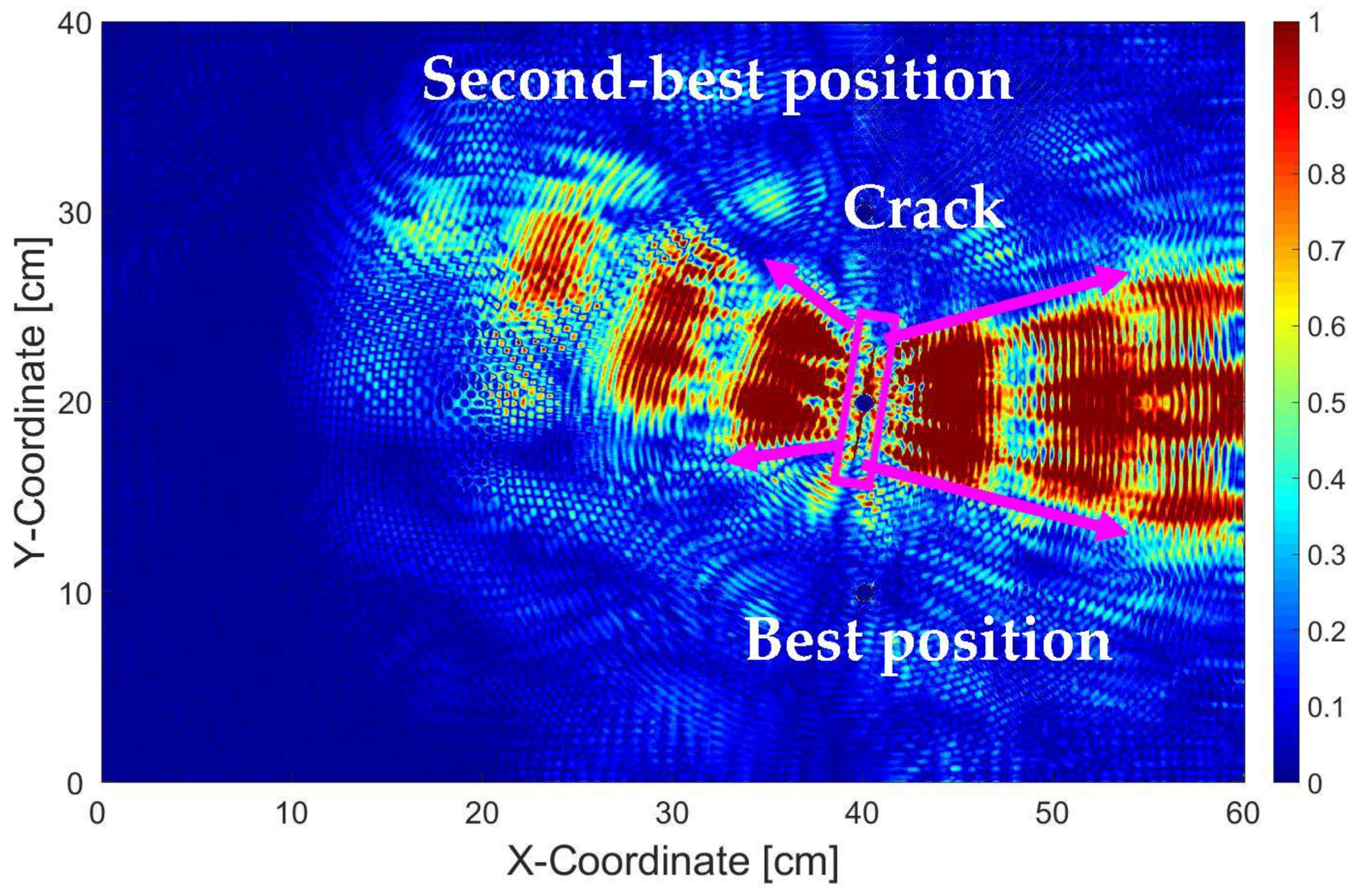
In order to demonstrate that the image processing algorithm also works for a different case of simulations, we slightly modified the case for the (a) the critical crack length to 30 mm, and (b) the orientation of the crack by 8°. The whole procedure was repeated, and the results are depicted in Figure 8 and Figure 9, respectively.
From Figure 8, it can be seen that the areas with higher pixel intensity (colored in red with value between 0.7 and 1) is smaller than those of Figure 7. This is absolutely normal, since the wave perturbation at the crack front due to a crack length of 30 mm is smaller than those of 60 mm.
Meanwhile from Figure 9, it can be seen that the crack orientation changes the direction of the reflected wave scatter and it is still conform with Snell’s law. However, it does not change the orientation of areas where the wave scatter is not present. After cross validating with the original simulation data, it can be confirmed that angled crack only heavily influences the reflected wave scatter portion, but not the missing scatter portion (Figure 10a,b, marked in yellow).
For current work, we have demonstrated a new efficient method based on an additive color model to find the best two locations for placing the sensor. However, the number of sensors that are allocated for every case can be adjusted according to the manufacturer and/or operator requirement to achieve required crack detectability. Furthermore, not only the number of sensors, but also the excitation frequency can be changed depending on the size of the critical crack that must be detected. A higher frequency means a shorter wavelength, and this would mean the wave will be able to interact with smaller critical crack. However, such a higher frequency Lamb wave will also be more quickly attenuated than the lower frequency Lamb wave. Therefore, in order to stabilize the SHM network performance, more sensors will be required. Nevertheless, when more sensors are employed, higher procurement costs are also expected due to more weight, more data processing capability, etc. We regard this as the classical trade-off between SHM investment cost and SHM network reliability and would like to pass this decision back to the aircraft manufacturer or operator according to their needs.
5. Conclusions
In this work, we have demonstrated a novel technique to design the sensor network topology for hotspot SHM by using differential images and blob detection algorithm. While our image processing technique does not allow a quantitative approach to observe the nodal displacement, i.e., displacement from every single FE node, we believe this technique offers a more holistic view (Figure 7) of where to place the PZT sensors on the structure to be monitored.
Also, with this technique we think that the sensor placement can be done more quickly without exhaustive data processing from simulation file for each surface while not sacrificing too much spatial resolution. In practice, even the extracted nodal data from the simulation must be interpolated, since in reality a PZT sensor would always occupy more than a single node (e.g., a typical PZT in our lab has a diameter of 1 cm, so would theoretically occupy about 78 FE nodes). Therefore, as a concluding remark, we hope this technique will help further research in sensor placement.
Supplementary Materials
The source code in MATLAB and all the wave propagation images being involved can be downloaded in the author’s personal repository (https://github.com/vewald/sensorplacement) and 4TU website (https://data.4tu.nl/repository/uuid:1fcc9e01-b339-4e75-b92a-2e40f3b660cf).
Acknowledgments
The project is funded by the TKI Smart Sensing for Aviation project of Delft University of Technology, Netherlands sponsored by the Dutch Ministry of Economic Affairs under the ‘Topsectoren’ Policy for High-Tech Systems and Materials.
Author Contributions
Vincentius Ewald designed and performed the experiments and wrote the paper draft. Roger M. Groves is daily supervisor of Vincentius Ewald. He critically evaluated the experimental design and results and corrected the paper draft. Rinze Benedictus is the doctoral promotor of Vincentius Ewald and tracks his overall scientific output.
Conflicts of Interest
The authors declare no conflict of interest.
References
- Hellier, C. Handbook of Nondestructive Evaluation, 2nd ed.; McGraw Hill Professional: New York, NY, USA; Chicago, IL, USA; London, UK; Madrid, Spain, 2003. [Google Scholar]
- Gopalakrishnan, S.; Ruzzene, M.; Hanagud, S. Computational Techniques for Structural Health Monitoring; Springer: London, UK; Dordrecht, The Netherlands; Heidelberg, Germany; New York, NY, USA, 2011. [Google Scholar]
- Haldar, A. Health Assessment of Engineered Structures—Bridges, Buildings and Other Infrastructures; World Scientific Publishing Co. Pte. Ltd.: Singapore, Singapore, 2013. [Google Scholar]
- Rajabzadeh, A.; Hendriks, R.C.; Heusdens, R.; Groves, R.M. Classification of Composite Damage from FBG Load Monitoring Signals. In Proceedings of the SPIE Conference Smart Structures and Materials + Nondestructive Evaluation and Health Monitoring, Denver, CO, USA, 25–29 March 2017. [Google Scholar]
- Kahandawa, G.C.; Epaarachchi, J.; Wang, H.; Lau, K.T. Use of FBG Sensors for SHM in Aerospace Structures. J. Photonic Sens. 2012, 2, 203–214. [Google Scholar] [CrossRef] [Green Version]
- Wilcox, P.D.; Lowe, M.; Cawley, P. Long Range Lamb Wave Inspection: The Effect of Dispersion and Modal Selectivity. Rev. Prog. Quant. Nondestruct. Eval. 1999, 18, 151–158. [Google Scholar]
- Edalati, K.; Kermani, A.; Naderi, B.; Panahi, B. Defects Evaluation in Lamb Wave Testing of Thin Plates. In Proceedings of the 3rd Middle East Non-Destructive Testing Conference & Exhibition (MENDT), Manama, Bahrain, 27–30 November 2005. [Google Scholar]
- Kuznetsov, S.; Ozolinsh, E.; Ozolinsh, I.; Pavelko, I.; Pavelko, V.; Wevers, M.; Pfeiffer, H. Lamb Wave Interaction with a Fatigue Crack in a Thin Sheet of Al2024-T3. In Proceedings of the EU Project Meeting on AISHA, Leuven, Belgium, June 2007. [Google Scholar]
- Wilcox, P.D.; Lowe, M.; Cawley, P. Mode and Transducer Selection for Long Range Lamb Wave Inspection. J. Intell. Mater. Syst. Struct. 2001, 12, 553–565. [Google Scholar] [CrossRef]
- Cobb, R.G.; Liebst, B.S. Sensor Placement and Structural Damage Identification from Minimal Sensor Information. AIAA J. 1997, 35, 369–374. [Google Scholar] [CrossRef]
- Shi, Z.Y.; Law, S.S.; Zhang, L.M. Optimum Sensor Placement for Structural Damage Detection. J. Eng. Mech. 2000, 126, 1173–1179. [Google Scholar] [CrossRef]
- Kripakaran, P.; Saitta, S.; Ravibndran, S.; Smith, I.F.C. Optimal Sensor Placement for Damage Detection. In Proceedings of the 18th International Workshop on Database and Expert System Applications, Regensburg, Germany, 3–7 September 2007. [Google Scholar]
- Li, B.; Wang, D.; Wang, F.; Ni, Y.Q. High Quality Sensor Placement for SHM Systems: Refocusing on Application Demands. In Proceedings of the INFOCOM IEEE Conference on Computer Communications, San Diego, CA, USA, 14–19 March 2010. [Google Scholar]
- Fendzi, C.; Morel, J.; Rébillat, M.; Guskov, M.; Mechbal, N.; Coffignal, G. Optimal Sensor Placement to Enhance Damage Detection in Composite Plates. In Proceedings of the 7th European Workshop on Structural Health Monitoring (EWSHM), Nantes, France, 8–11 July 2014. [Google Scholar]
- Haynes, C. Effective Health Monitoring Strategies for Complex Structures. Ph.D. Thesis, University of California San Diego (UCSD), San Diego, CA, USA, 2014. [Google Scholar]
- Flynn, E.B.; Todd, M. A Bayesian Approach to Optimal Sensor Placement for Structural Health Monitoring with Application to Active Sensing. Mech. Syst. Signal Process. 2010, 24, 891–903. [Google Scholar] [CrossRef]
- Sun, H.; Büyüköztürk, O. Optimal Sensor Placement in Structural Health Monitoring Using Discrete Optimization. Smart Mater. Struct. 2015, 25, 125034. [Google Scholar] [CrossRef]
- Yi, T.H.; Li, H.N.; Gu, M. Optimal Sensor Placement for Structural Health Monitoring Based on Multiple Optimization Strategies. J. Struct. Des. Tall Spec. Build. 2011, 20, 881–900. [Google Scholar] [CrossRef]
- Zhao, J.; Wu, X.; Sun, Q.; Zhang, L. Optimal Sensor Placement for a Truss Structure Using Particle Swarm Optimisation Algorithm. Int. J. Acoust. Vib. 2017, 22, 439–447. [Google Scholar] [CrossRef]
- Shan, D.; Wan, Z.; Qiao, L. Optimal Sensor Placement for Long-span Railway Steel Truss Cable-stayed Bridge. In Proceedings of the 3rd International Conference on Measuring Technology and Mechatronics Automation (ICMTMA), Shanghai, China, 6–7 January 2011. [Google Scholar]
- Capellari, G.; Chatzi, E.; Mariani, S. Optimal Sensor Placement through Bayesian Experimental Design: Effect of Measurement Noise and Number of Sensors. In Proceedings of the 3rd International Electronic Conference on Sensors and Applications, 15–30 November 2016. [Google Scholar]
- Thiene, M.; Sharif Khodaei, Z.; Aliabadi, M.H. Optimal Sensor Placement for Maximum Area Coverage for Damage Localization in Composite Structures. Smart Mater. Struct. 2016, 25, 095037. [Google Scholar] [CrossRef]
- Venkat, R.S.; Boller, C.; Qiu, L.; Ravi, N.B.; Mahapatra, D.R.; Chakraborty, N. Integrated Approach to Demonstrate Optimum Sensor Positions in a Guided Wave Based SHM System Using Numerical Simulation. In Proceedings of the 8th International Symposium on NDT in Aerospace, Bangalore, India, 3–5 November 2016. [Google Scholar]
- Lamb, H. On Waves in an Elastic Plate. R. Soc. Lond. Ser. A 1917, 93, 114–128. [Google Scholar] [CrossRef]
- Döring, D. Luftgekoppelter Ultraschall und Geführte Wellen für die Anwendung in der Zerstörungsfreien Werkstoffprüfung. Ph.D. Thesis, Universität Stuttgart, Stuttgart, Germany, 2011. [Google Scholar]
- Pant, S. Lamb Wave Propagation and Material Characterization of Metallic and Composite Aerospace Structures for Improved Structural Health Monitoring (SHM). Ph.D. Thesis, Carleton University, Ottawa, ON, Canada, 2014. [Google Scholar]
- Hosseini, S.M.H.; Gabbert, U. Analysis of Guided Lamb Wave Propagation (GW) in Honeycomb Sandwich Panels. Proc. Appl. Math. Mech. 2010, 10, 11–14. [Google Scholar] [CrossRef]
- Gomez, P.; Fernández, J.P.; Garcia, P.D. Lamb Waves and Dispersion Curves in Plates and its Applications in NDE Experiences Using COMSOL Multiphysics Pablo Gómez. In Proceedings of the COMSOL Conference, Stuttgart, Germany, 26–28 October 2011. [Google Scholar]
- Harris, C.E.; Starnes, J.H., Jr.; Shuart, M.J. Advanced Durability and Damage Tolerance Design and Analysis Methods for Composite Structures—Lesson Learned from NASA Technology Development Programs; NASA Langley Research Center: Hampton, VA, USA, 2003. [Google Scholar]
- Pugno, N.; Ciavarella, M.; Cornetti, P.; Carpinteri, A. A Generalized Paris’ Law for Fatigue Crack Growth. J. Mech. Phys. Solids 2006, 54, 1333–1349. [Google Scholar] [CrossRef]
- Schors, J.; Harbich, K.W.; Hentschel, M.P.; Lange, A. Non-Destructive Micro Crack Detection in Modern Materials. In Proceedings of the 9th European Conference of Non-Destructive Testing (ECNDT), Berlin, Germany, 25–29 September 2006. [Google Scholar]
- Wang, X.S.; Wua, B.S.; Wang, Q.Y. Online SEM Investigation of Microcrack Characteristics of Concretes at Various Temperatures. Cem. Concr. Res. 2005, 35, 1385–1390. [Google Scholar] [CrossRef]
- Milella, PP. Fatigue and Corrosion in Metals; Springer: Milan, Italy; Heidelberg, Germany; New York, NY, USA; Dordrecht, The Netherlands; London, UK, 2013. [Google Scholar]
- McMaster, R.C. Nondestructive Testing Handbook, 3rd ed.; Visual Testing (VT); American Society for Nondestructive Testing: Columbus, OH, USA, 2010; Volume 9. [Google Scholar]
- Gilchrist, M.D. Attenuation of Ultrasonic Rayleigh-Lamb Waves by a Symmetrical Embedded Crack in an Elastic Plate. J. Appl. Math. Mech. 1999, 79, 497–498. [Google Scholar]
- Wang, Q.; Su, Z. Crack Diagnosis and Monitoring Method Using Linear-Phased PZT Sensor Array. In Proceedings of the 2nd International Conference of Structural Health Monitoring and Integrity Management (ICSHMIM), Nanjing, China, 24–26 September 2014. [Google Scholar]
- Iesulauro, E.; Ingraffea, A.R.; Arwade, S.; Wawrzynek, P.A. Simulation of Grain Boundary Decohesion and Crack Initiation in Aluminum Microstructure Models. ASTM J. Fatigue Fract. Mech. 2003, 33, 715–728. [Google Scholar]
- Richard, H.A.; Sander, M. Technische Mechanik: Festigkeitslehre (2. Auflage); Vieweg+Teubner: Wiesbaden, Germany, 2008. [Google Scholar]
- Taltavull, A.; Qiu, L.; Venkat, R.S.; Dürager, C.; Boller, C.; Ren, Y.Q.; Yuan, S. Simulation, Realization and Validation of Guided Wave SHM System Solutions for Aircraft Metallic Structural Repairs. In Proceedings of the 11th International Workshop on Structural Health Monitoring (IWSHM), Stanford, CA, USA, 12–14 September 2017. [Google Scholar]
- Duczek, S.; Joulaian, M.; Düster, A.; Gabbert, U. Numerical Analysis of Lamb Waves Using the Finite and Spectral Cell Methods. Int. J. Numer. Methods Eng. 2014, 99, 26–53. [Google Scholar] [CrossRef]
- Zienkiewicz, O.C.; Taylor, R.L.; Zhu, J.Z. Finite Element Method—Its Basis and Fundamentals, 6th ed.; Elsevier Butterworth-Heinemann: Oxford, UK; Burlington, NJ, USA, 2005. [Google Scholar]
- Wriggers, P. Nonlinear Finite Element Methods; Springer: Berlin/Heidelberg, Germany, 2008. [Google Scholar]
- Ewald, V. Post-Design Damage Tolerance Enhancement of Primary Aircraft Structures by Ultrasonic Lamb Wave Based Structural Health Monitoring (SHM) System. Master’s Thesis, Universität des Saarlandes, Saarbrücken, Germany, 2015. [Google Scholar]
- Cerniglia, D.; Pantano, A.; Montinaro, N. 3D Simulations and Experiments of Guided Wave Propagation in Adhesively Bonded Multi-Layered Structures. J. NDT E Int. 2010, 43, 527–535. [Google Scholar] [CrossRef]
- Gopalakrishnan, S.; Chakraborty, A.; Mahapatra, D.R. Spectral Finite Element Method—Wave Propagation, Diagnostics and Control in Anisotropic and Inhomogeneous Structures; Springer: London, UK, 2008. [Google Scholar]
- Elert, G. Color; The Physics Hypertextbook. Available online: https://physics.info/color/ (accessed on 3 February 2018).
- Lightshot Program. Available online: https://app.prntscr.com/en/index.html (accessed on 3 February 2018).
- MATLAB IPT Documentation. Available online: https://de.mathworks.com/help/images/ (accessed on 3 February 2018).
- Kong, H.; Akakin, H.C.; Sarma, S.E. A Generalized Laplacian of Gaussian Filter for Blob Detection and Its Applications. IEEE Trans. Cybern. 2013, 43, 1719–1733. [Google Scholar] [CrossRef] [PubMed]
- Lindeberg, T. Feature Detection with Automatic Scale Selection; Technical Report ISRN KTH/NA/P–96/18–SE; Kungliga Tekniska Högskolan (KTH): Stockholm, Sweden, 1998. [Google Scholar]
- Heinze, C.; Sinapius, M.; Wierach, P. Lamb Wave Propagation in Complex Geometries—Model Reduction with Approximated Stiffeners. In Proceedings of the 7th European Workshop on Structural Health Monitoring (EWSHM), Nantes, France, 8–11 July 2014. [Google Scholar]
Figure 1.
3-bit additive color mixing.

Figure 2.
Lamb wave propagation at the step time of 30 μs after excitation in an Al-7075-T6 plate with dimensions of 200 mm × 200 mm × 1 mm. (shown in ABAQUS GUI Viewer. Note that there is no ‘unit’ in ABAQUS). The default scientific notation of displacement magnitude ‘e-09’ means [nm]. Displacement magnitude shown in grey color signifies displacement above 7.989 nm.

Figure 3.
(a–h) Lamb wave propagation at t = 100 and 125 μs in Al 7075 Plate with different crack lengths.
Figure 3.
(a–h) Lamb wave propagation at t = 100 and 125 μs in Al 7075 Plate with different crack lengths.

Figure 4.
(a) Differential image of (3h − 3e); (b) Differential image of (3e − 3h); (c) Inverse of added image (4a + 4b); (d) Inverse of fused image (4a + 4b).
Figure 4.
(a) Differential image of (3h − 3e); (b) Differential image of (3e − 3h); (c) Inverse of added image (4a + 4b); (d) Inverse of fused image (4a + 4b).

Figure 5.
(a) 8-pixel connectivity; (b) 4-pixel connectivity.

Figure 6.
Detected blobs at (a) 100 μs, (b) 125 μs, (c) 150 μs, and (d) 175 μs. The largest and second-largest blobs are marked in red and green, respectively. Arrows indicate the direction of movement of the blobs.
Figure 6.
Detected blobs at (a) 100 μs, (b) 125 μs, (c) 150 μs, and (d) 175 μs. The largest and second-largest blobs are marked in red and green, respectively. Arrows indicate the direction of movement of the blobs.

Figure 7.
Fused image of Figure 6a–d.
Figure 7.
Fused image of Figure 6a–d.

Figure 8.
Fused image of differential images of 30 mm crack.

Figure 9.
Fused image of differential images of 60 mm crack with 8° orientation.

Figure 10.
Lamb wave propagation at (a) t = 100 and (b) 125 μs in Al 7075 Plate.


Table 1.
Subtractive mathematical operations for a 3-bit additive color model.
| y–x | R | G | B | C | M | Y | K |
| R | K | R | R | R | K | K | R |
| G | G | K | G | K | G | K | G |
| B | B | B | K | K | K | B | B |
| C | C | B | G | K | G | B | C |
| M | B | M | R | R | K | B | M |
| Y | G | R | Y | R | G | K | Y |
| K | K | K | K | K | K | K | K |
R = Red; G = Green; B = Blue; C = Cyan; M = Magenta; Y = Yellow; K = Black.
Table 2.
X, Y—Area and coordinates of the largest and second largest centroid.
| Time Frame | Largest Centroid | Second-Largest Centroid | ||||
|---|---|---|---|---|---|---|
| (pixel) | (mm) | Area (pixel) | (pixel) | (mm) | Area (pixel) | |
| 100 μs | 888,403 | 440,200 | 15,910 | 716,403 | 355,200 | 12,917 |
| 125 μs | 1,031,402 | 511,199 | 29,535 | 582,404 | 289,200 | 18,794 |
| 150 μs | 1,154,402 | 572,199 | 27,067 | 445,401 | 221,200 | 8808 |
| 175 μs | 1,111,405 | 551,201 | 24,214 | 304,402 | 151,199 | 7949 |
Units are in pixel and mm. Total area is in pixel. Average resolution is 2 pixel/mm.
© 2018 by the authors. Licensee MDPI, Basel, Switzerland. This article is an open access article distributed under the terms and conditions of the Creative Commons Attribution (CC BY) license (http://creativecommons.org/licenses/by/4.0/).
Share and Cite
MDPI and ACS Style
Ewald, V.; Groves, R.M.; Benedictus, R. Transducer Placement Option of Lamb Wave SHM System for Hotspot Damage Monitoring. Aerospace 2018, 5, 39. https://doi.org/10.3390/aerospace5020039
AMA Style
Ewald V, Groves RM, Benedictus R. Transducer Placement Option of Lamb Wave SHM System for Hotspot Damage Monitoring. Aerospace. 2018; 5(2):39. https://doi.org/10.3390/aerospace5020039
Chicago/Turabian StyleEwald, Vincentius, Roger M. Groves, and Rinze Benedictus. 2018. "Transducer Placement Option of Lamb Wave SHM System for Hotspot Damage Monitoring" Aerospace 5, no. 2: 39. https://doi.org/10.3390/aerospace5020039
Note that from the first issue of 2016, this journal uses article numbers instead of page numbers. See further details here.