AEROM: NASA’s Unsteady Aerodynamic and Aeroelastic Reduced-Order Modeling Software

Abstract

The origins, development, implementation, and application of AEROM, NASA’s patented reduced-order modeling (ROM) software, are presented. Using the NASA FUN3D computational fluid dynamic (CFD) code, full and ROM aeroelastic solutions are computed at several Mach numbers and presented in the form of root locus plots. The use of root locus plots will help reveal the aeroelastic root migrations with increasing dynamic pressure. The method and software have been applied successfully to several configurations including the Lockheed-Martin N+2 supersonic configuration and the Royal Institute of Technology (KTH, Sweden) generic wind-tunnel model, among others. The software has been released to various organizations with applications that include CFD-based aeroelastic analyses and the rapid modeling of high-fidelity dynamic stability derivatives. We present recent results obtained from the application of the method to the AGARD 445.6 wing that reveal several interesting insights.

1. Introduction

In the early days, aeroelasticians typically used linear methods to compute unsteady aerodynamic responses and subsequent aeroelastic analyses [1]. These aeroelastic analyses were usually presented in the form of aeroelastic root locus plots as a function of either dynamic pressure or velocity, or velocity-damping-frequency (V-g-f) plots. These plots were generated rapidly and provided significant amount of insight regarding the aeroelastic mechanisms involved.

With the subsequent development of CFD methods, the analysis of complex, nonlinear flows, and their effect on the aeroelastic response, became a reality. While CFD tools are quite powerful and provide significant insight regarding flow physics, the significant increase in computational cost (time and CPU dollars) has had an effect on how aeroelastic analyses are performed. One side-effect of the increase in computational cost is the desire to keep the number of compute iterations, and the total number of solutions generated, at a minimum. Results are, therefore, computed for a small number of dynamic pressures (per Mach number) with only a few cycles computed per dynamic pressure. A second side-effect is that the resultant time histories of each generalized coordinate cannot be directly used to identify the governing aeroelastic mechanisms at work, as was the case for the classical linear methods. The recent development of reduced-order modeling (ROM) methods [2,3,4], provides a tool for the rapid generation of traditional aeroelastic tools such as the root-locus plots.

The origin of this method started with the author’s PhD dissertation [5] and related publications [6,7]. An important conceptual development first presented in these references consists of the realization that unsteady aerodynamic impulse responses do, in fact, exist and can be computed using CFD methods. This concept is an important point that is claimed to be not realizable in some of the classic aeroelastic references. The reason for this discrepancy is actually quite simple as it relates to the difference between a continuous-time and a discrete-time impulse function.

For a continuous-time system, it is well known that the impulse input function is the Dirac delta function. This function serves the continuous domain well, in particular in the solution of ordinary and partial differential equations. However, its application to a discrete-time system such as a CFD-based solution, is not clear, thus the belief that an impulse input cannot be applied to a CFD code. Therefore, if an impulse input cannot be applied to a CFD code, then an unsteady aerodynamic response cannot be identified or realized.

An important contribution by the author [5] is the realization that in order to properly identify the unsteady aerodynamic impulse response using a CFD code, a discrete-time impulse input, also known as the unit sample input in discrete-time theory, is the proper function to use and not the Dirac delta function. The theory of Digital Signal Processing (DSP) demonstrates that a unit sample input is much simpler to apply and less complex to interpret than the Dirac delta function. These results proved the existence and realizability of a unit unsteady aerodynamic impulse (sample) response via a CFD code.

In the world of structural dynamics and modal identification, the concept of a structural dynamic impulse response is clear and well understood. As a result, various modal identification techniques consist of the identification of these responses and a subsequent realization of a system that captures the structural dynamic system of interest. Having familiarity with one of these methods by the name of Eigensystem Realization Algorithm (ERA) [8]/System Observer Controller Identification Toolbox (SOCIT) [9], the author applied the modal identification technique, previously limited to structural dynamic systems, to that of identifying an unsteady aerodynamic system via the identification of the unsteady aerodynamic impulse responses. Once the concept of a discrete-time unsteady aerodynamic impulse response was mathematically validated, the application of ERA/SOCIT became quite logical [10]. These results [10] represent the first time that the ERA/SOCIT algorithms were used for the identification of unsteady aerodynamic systems. It is valuable to point out that this method is now being applied at several organizations around the world [11,12,13,14,15,16]. In the area of fluid modal decompositions using, primarily, the Proper Orthogonal Decomposition (POD), the application of the ERA algorithm has become standard, with an initial appearence in the literature by Ma, Ahuja, and Rowley [17].

Following these fundamental advances, linearized, unsteady aerodynamic state-space models using the CFL3Dv6 [18] code were introduced [19]. The unsteady aerodynamic state-space models were coupled with a structural model within a MATLAB/SIMULINK^TM environment for rapid calculation of aeroelastic responses, including the prediction of flutter. A comparison of the aeroelastic responses computed using the aeroelastic simulation ROM with the aeroelastic responses computed using the CFL3Dv6 code showed excellent correlation.

Initially, the excitation of one structural mode at a time was used to generate the unsteady aerodynamic state-space model [19]. However, the one-mode-at-a-time method becomes prohibitively expensive for more realistic cases where there exist a large number of modes. Methods based on the simultaneous application of structural modes as CFD input [20] have been proposed, greatly reducing the computational cost for a large number of structural modes. The method developed by Silva [2] enables the simultaneous excitation of the structural modes using orthogonal functions. These methods require only a single CFD solution and are, therefore, independent of the number of structural modes.

Static and matched-point aeroelastic solutions, using a ROM, have also been developed [2,21] and implemented in the FUN3D [22,23,24,25] CFD code. Methods for generating root locus plots of the ROM aeroelastic system have also been developed [3]. Applications of these methods include fixed-wing and launch vehicle configurations [4]. This paper will discuss the application of these methods to three configurations: a low-boom configuration, a full-span wind-tunnel model, and the AGARD 445.6 wing.

The AEROM software was granted a patent (November, 2011), Patent No. 8,060,350. The software has been distributed to the Air Force Research Laboratory, the Boeing Corporation, and the CFD Research Corporation.

2. Computational Methods

2.1. FUN3D Code

The FUN3D CFD code is the NASA-developed, RANS unstructured mesh solver used for this study. The code solves the Euler or Navier-Stokes equations with various turbulence models. Due to the differences between structural and CFD meshes, an interpolation between the two domains is required. Mode shape displacements are used to compute physical deformations that are then used to deform the mesh within FUN3D. Pressures are computed at each time step and then projected onto each mode shape to provide generalized aerodynamic forces (GAFs). These GAFs are then used by the linear state-space structural model (within FUN3D) to compute the next set of modal deformations for the next iteration.

2.2. System Identification Method

The development of algorithms such as the ERA [8] and the Observer Kalman Identification (OKID) [26] Algorithm have enabled the realization of discrete-time state-space models, used up to this point, primarily for structural dynamic modal identification. These algorithms use the Markov parameters (discrete-time impulse responses) of the systems of interest to perform the required state-space realization. The SOCIT contains these algorithms and others related to this methodology.

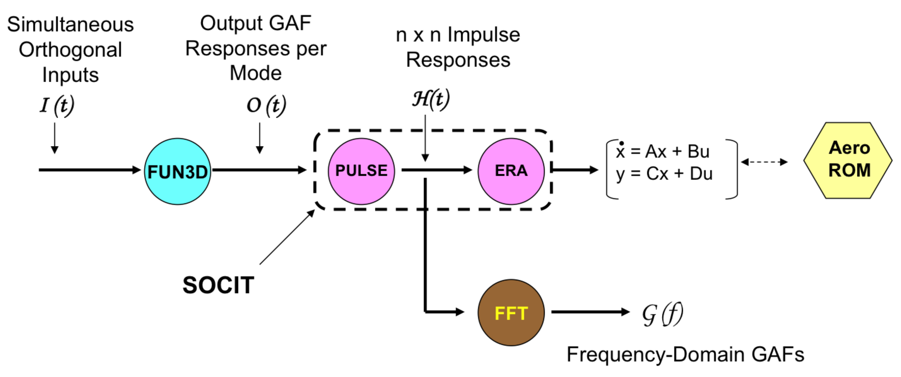
The PULSE algorithm is used to extract individual input/output impulse responses from simultaneous input/output responses. For a four-input/four-output system, for example, the PULSE algorithm is used to extract the individual sixteen (all combinations of four inputs and four outputs) impulse responses that define this input/output system. The individual sixteen impulse responses are then processed via the ERA in order to generate a four-input/four-output, discrete-time, state-space model. A brief summary of the basis of this algorithm follows.

A finite dimensional, discrete-time, linear, time-invariant dynamical system can be defined as

$$x(k+1)=Ax\left(k\right)+Bu\left(k\right)$$

(1)

$$y\left(k\right)=Cx\left(k\right)+Du\left(k\right)$$

(2)

where x is an n-dimensional state vector, u an m-dimensional control input, and y a p-dimensional output or measurement vector with k being the discrete time index. The transition matrix, A, characterizes the dynamics of the system. The goal of system realization is to generate constant matrices (A, B, C, D) such that the output responses of a given system due to a particular set of inputs is reproduced by the discrete-time state-space system described above.

The time-domain values of the discrete-time impulse responses of the system are also known as the Markov parameters and are defined as

$$Y\left(k\right)=C{A}^{k-1}B+D$$

(3)

with A an (n × n) matrix, B an (n × m) matrix, C a (p × n) matrix, and D an (p × m) matrix. The ERA algorithm generates the generalized Hankel matrix, consisting of the discrete-time impulse responses and then uses the singular value decomposition (SVD) to compute the (A, B, C, D) matrices. This is the method by which the ERA is applied to unsteady aerodynamic impulse responses to construct unsteady aerodynamic state-space models.

2.3. Simultaneous Excitation Input Functions

Clearly, the nonlinear unsteady aerodynamic responses of a flexible vehicle comprise a multi-input/multi-output (MIMO) system with respect to the modal inputs and generalized aerodynamic outputs. In the situation where the goal is the simultaneous excitation of such a MIMO system, system identification techniques [27,28,29] indicate that the input excitations must be properly defined in order to generate stable and accurate input/output models of the system. A critical requirement is that these input excitations be different, mathematically, from each other. If identical excitation inputs are applied simultaneously, the task of separating the various contributions of each input becomes nearly impossible. This effect makes it practically impossible for a system identification algorithm to extract the individual impulse responses for each input/output pair. It is essential that the individual impulse responses for each input/output pair be properly identified so that an accurate model can be generated.

These unsteady aerodynamic impulse responses are the time-domain generalized aerodynamic forces (GAFs), critical to understanding unsteady aerodynamic behavior. The Fourier-transformed version of these GAFs are the frequency-domain GAFs, that provide an important link to more traditional frequency-domain-based unsteady aerodynamic analyses.

The question is how different should these excitation inputs be from each other and how can we quantify a level of difference between them? Orthogonality (linear independence) is the most precise mathematical method for guaranteeing the difference between signals. Using orthogonal functions as the excitation inputs provides a mathematical guarantee of the desired difference between inputs.

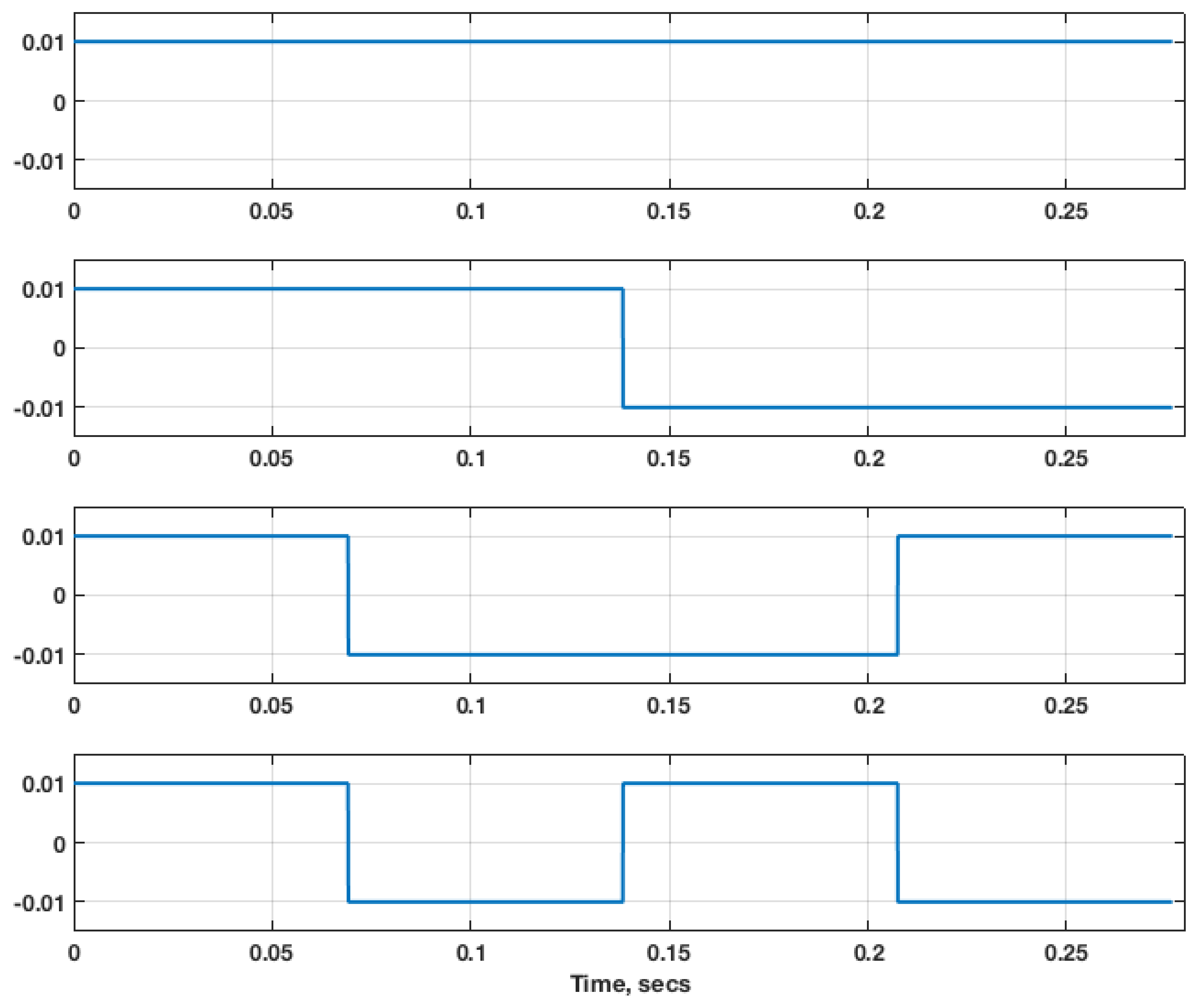
In a previous paper [2], four families of functions were investigated to efficiently identify a CFD-based unsteady aerodynamic state-space model. For the present paper, the Walsh family of orthogonal functions [30] are used, shown in Figure 1 for four modes. These functions are orthogonal and therefore provide a benefit in the system identification process as discussed above. Also, this family of functions consists of a combination of step functions, which have been shown to be well-suited for the identification of CFD-based unsteady aerodynamic ROMs.

3. ROM Development Processes

The ROM development process consists of two parts: the creation of the unsteady aerodynamic ROM and the creation of the structural dynamic ROM. The combination of the unsteady aerodynamic ROM with the structural dynamic ROM yields what is referred to as the aeroelastic simulation ROM.

The original unsteady aerodynamic ROM development process consisted of the excitation of one structural mode at a time per CFD solution. That approach is not practical for realistic configurations with a large number of modes. As mentioned above, an improved method has been developed and is described below.

3.1. Improved ROM Development Process

The improved simultaneous modal excitation ROM development process:

• Create as many orthogonal functions as the number of structural modes of interest;
• Starting from the restart of a steady rigid CFD solution, execute a single CFD solution using the orthogonal excitation inputs simultaneously, resulting in GAF responses due to these inputs;
• Identify the individual impulse responses from the responses computed in Step 2 using the PULSE algorithm;
• Using the ERA, convert the impulse responses from Step 3 into an unsteady aerodynamic state-space model;
• Using full-solution CFD results, compare with solutions generated using the model generated in Step 4;

Steps 1–4 of the improved process are presented in Figure 2.

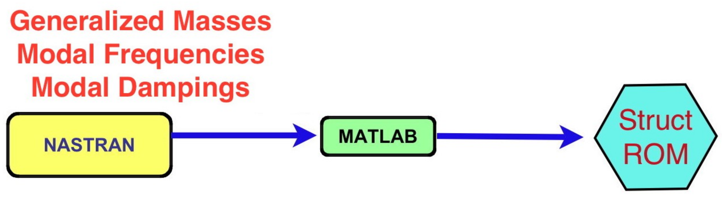
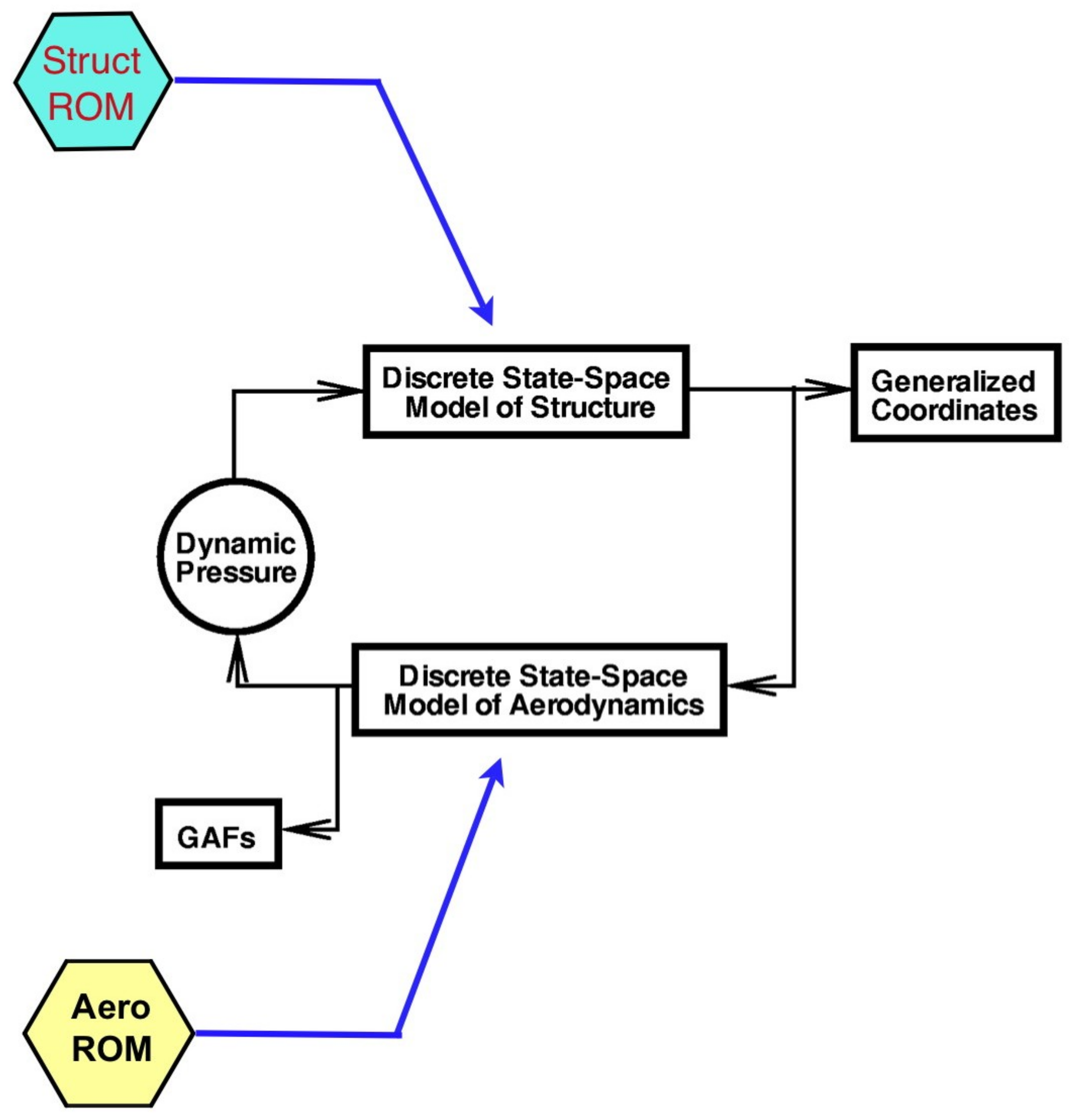
Using generalized mass, modal frequencies, and modal dampings from the finite element model (FEM), a state-space model of the structure is generated, referred to as the structural dynamic ROM (Figure 3). The unsteady aerodynamic and structural dynamic ROMs are combined to form an aeroelastic simulation ROM (see Figure 4). Root locus plots are then extracted from the aeroelastic simulation ROM.

For the original ROM process, the unsteady aerodynamic ROM was typically generated about a pre-selected static aeroelastic condition. Once the CFD-based converged static aeroelastic solution was obtained, the development of the unsteady aerodynamic ROM process was performed about that static aeroelastic condition. This approach would tend to limit the applicability of the unsteady aerodynamic ROM to the local neighborhood of that static aeroelastic condition.

In the early days, no method had been defined to enable the computation of a static aeroelastic solution using a ROM. These ROMs, based on a particular static aeroelastic condition were, therefore, limited to the prediction of dynamic responses about that condition. This included the methods by Raveh [31] and by Kim et al. [20]. The improved ROM method described above, however, consists of a ROM generated directly from a steady, rigid solution. Therefore, these improved ROMs can be used to predict static and dynamic aeroelastic solutions at any dynamic pressure [21]. All responses for the present results were computed from the restart of a steady, rigid FUN3D solution, bypassing the need (and the additional computational expense) of a static aeroelastic solution using FUN3D.

3.2. Error Minimization

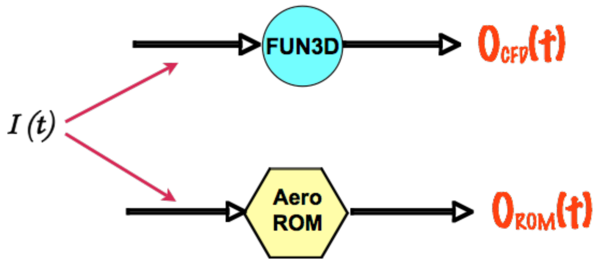
Error minimization consists of error quantification and error reduction. Error quantification is defined as the difference (error) between the full FUN3D solution due to the orthogonal input functions used (Walsh) and the unsteady aerodynamic ROM solution due to the same orthogonal input functions. This was identified in Step 5 in the previous subsection and is shown schematically in Figure 5. The outputs shown are GAF responses per mode. Within the system identification algorithms, there are parameters that can then be used to reduce the error (error reduction). These parameters include number of states and the record length of the identified pulse responses, for example. The maximum error is the largest error encountered per mode. Using the maximum error as the figure of merit, the parameters are varied until an acceptable ROM has been obtained.

4. Sample Results

A brief summary of results for three configurations is presented in this section. These configurations are the Lockheed-Martin N+2 low-boom supersonic configuration, the Royal Institute of Technology (KTH) generic fighter wind-tunnel model, and the AGARD 445.6 wing.

4.1. Low-Boom N+2 Configuration

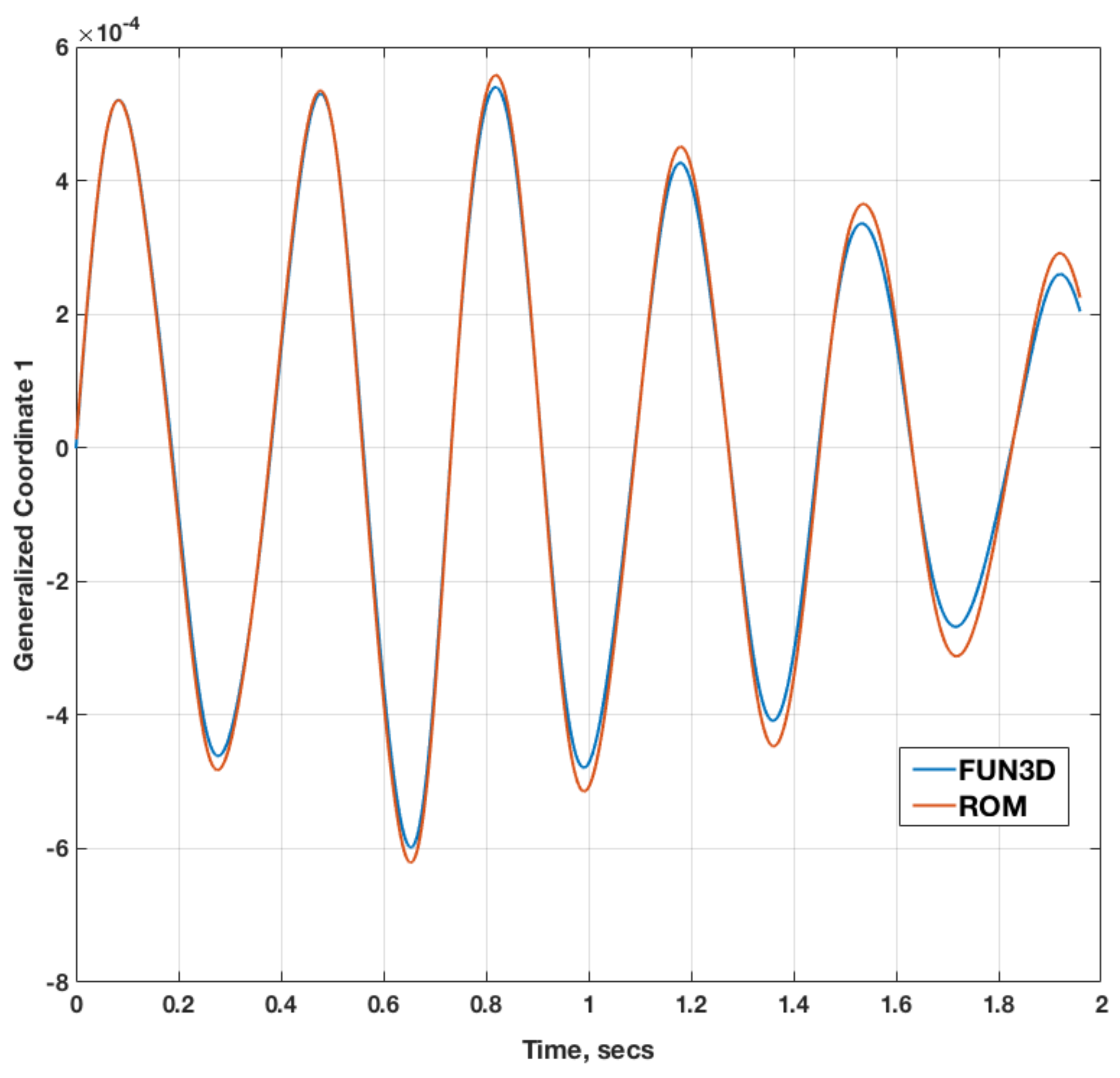
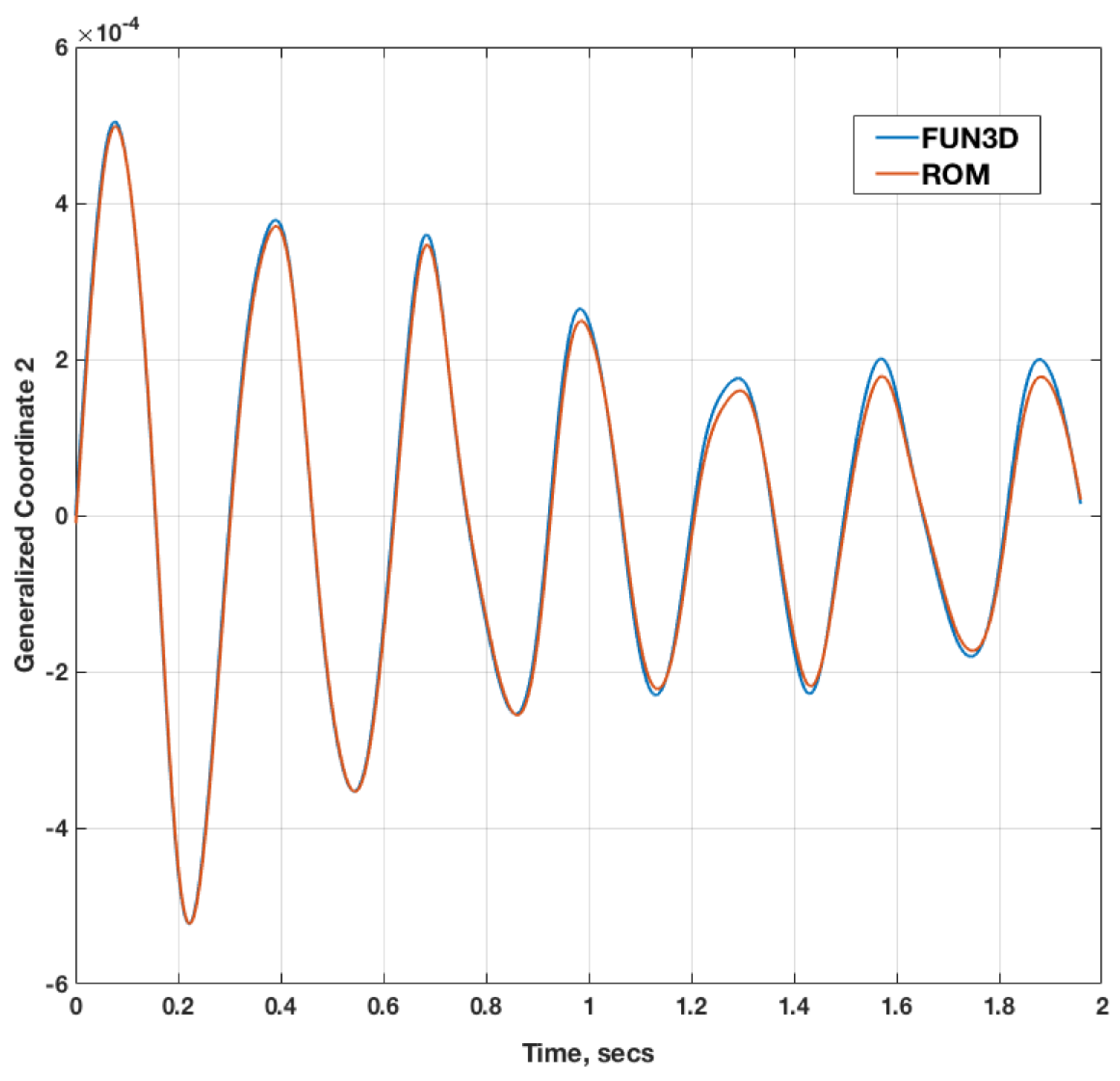
An artist’s rendering of the Lockheed-Martin N+2 low-boom supersonic configuration is presented in Figure 6. This configuration has been used extensively as part of a NASA research effort to address the technologies required for a low-boom aircraft, including aeroelastic effects. Presented in Figure 7 is a comparison of the dynamic aeroelastic responses of the time histories of the first mode generalized displacements from a full FUN3D aeroelastic solution and the ROM aeroelastic solution at a Mach number of 1.7 and a dynamic pressure of 2.149 psi. Presented in Figure 8 is a comparison of the dynamic aeroelastic responses of the time histories of the second mode generalized displacements from a full FUN3D aeroelastic solution and the ROM aeroelastic solution at the same condition. As can be seen, the results indicate an excellent level of correlation between the full FUN3D solutions and the ROM solutions. Similar results are obtained for all the other modes, indicating good confidence in the ROM.

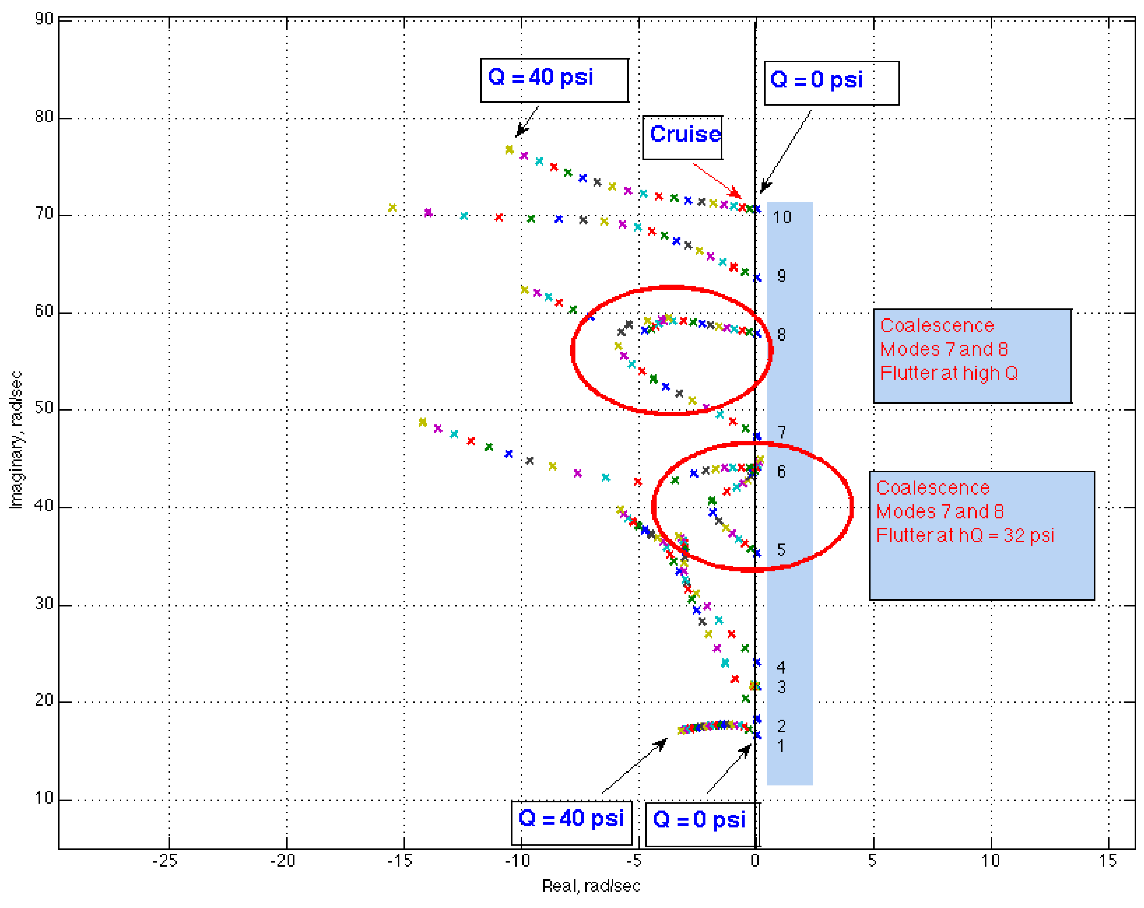
This ROM technology has the ability to rapidly generate an aeroelastic root locus plot that can reveal the aeroelastic mechanisms occurring at that flight condition. The aeroelastic root locus plot for the low-boom N+2 configuration at M = 1.7 is presented in Figure 9, revealing the aeroelastic mechanisms that affect this configuration. Each symbol represents the aeroelastic roots at a specific dynamic pressure, corresponding to a 2 psi increment in dynamic pressure.

In lieu of a ROM and its root locus solutions, multiple, expensive, and time consuming full FUN3D solutions would be required for each dynamic pressure of interest, with each solution requiring about two days. A full FUN3D analysis, at each dynamic pressure, requires two full FUN3D solutions: a static aeroelastic (∼10 h) and a dynamic aeroelastic (∼18 h) solution. Full FUN3D solutions for 20 dynamic pressures would require ∼560 h of compute time.

The ROM solutions, on the other hand, consist of one full FUN3D solution that is used to generate the ROM at that Mach number. For this particular example, a full FUN3D solution of 2400 time steps ran for three hours. This ROM solution is then used to rapidly generate a ROM that can then be used to generate all the aeroelastic responses at all dynamic pressures and the corresponding root locus plots.

4.2. KTH Generic Fighter

Two wind-tunnel models of the Saab JAS 39 Gripen were designed, built, and tested in the NASA Transonic Dynamics Tunnel (TDT) for flutter clearance in 1985 and 1986. A stability model was designed to be stiff, while incorporating proper scaling of both the mass and geometry. The other model, the flutter model, was also designed for proper scaling of structural dynamics, and was used for flutter testing with various external stores attached.

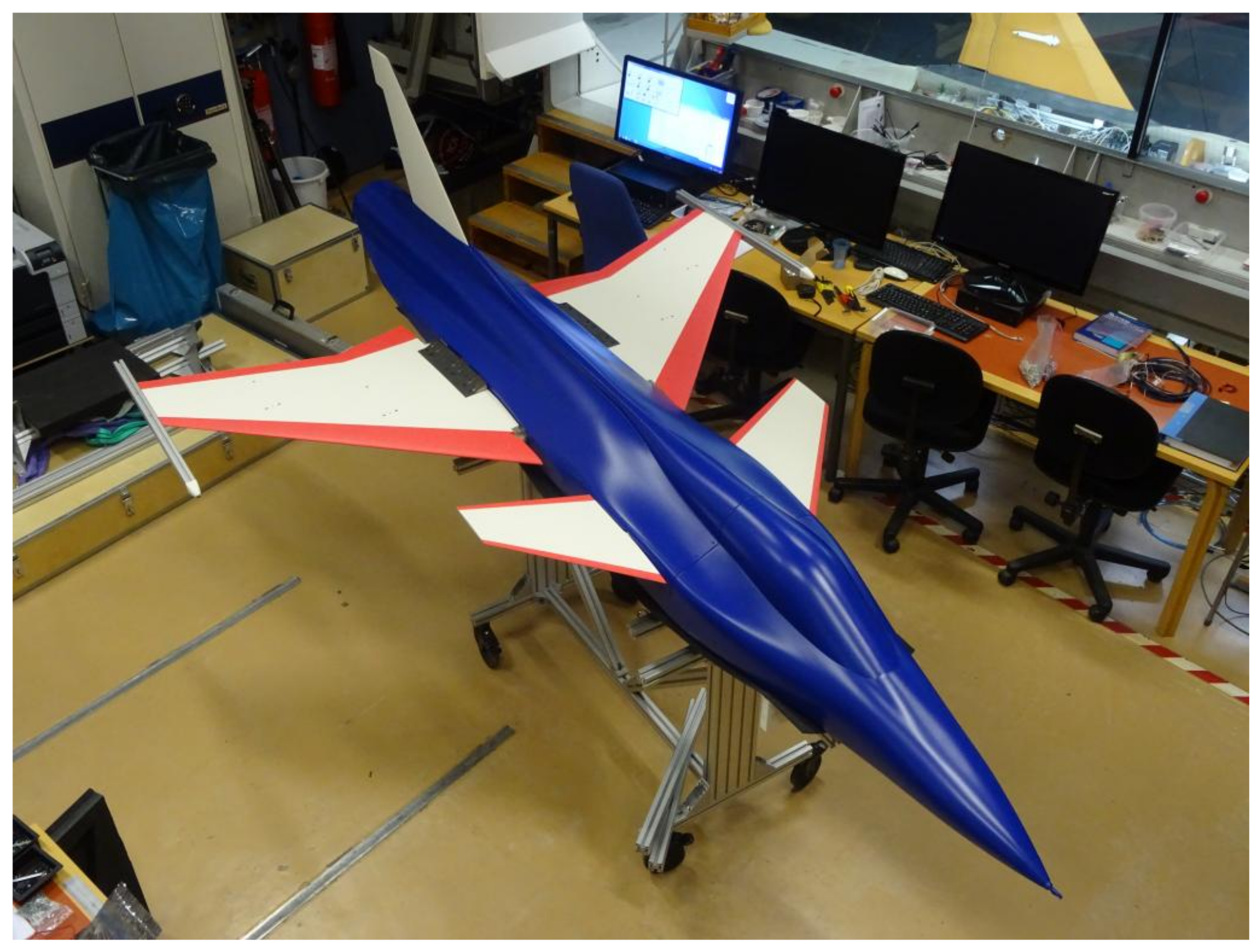
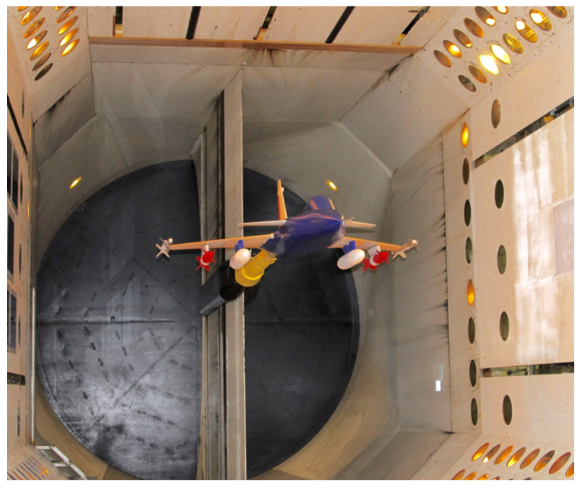
A generic fighter flutter-model version of these earlier models was selected for the collaborative wind-tunnel testing campaign between the KTH and NASA. Shown in Figure 10 is the new model, with a similar outer mold line (OML) to the Gripen, but modified into a more generic fighter configuration. Details regarding the design, fabrication, and instrumentation of the wind-tunnel model can be found in the reference paper [32]. Figure 11 shows the wind-tunnel model installed in the TDT.

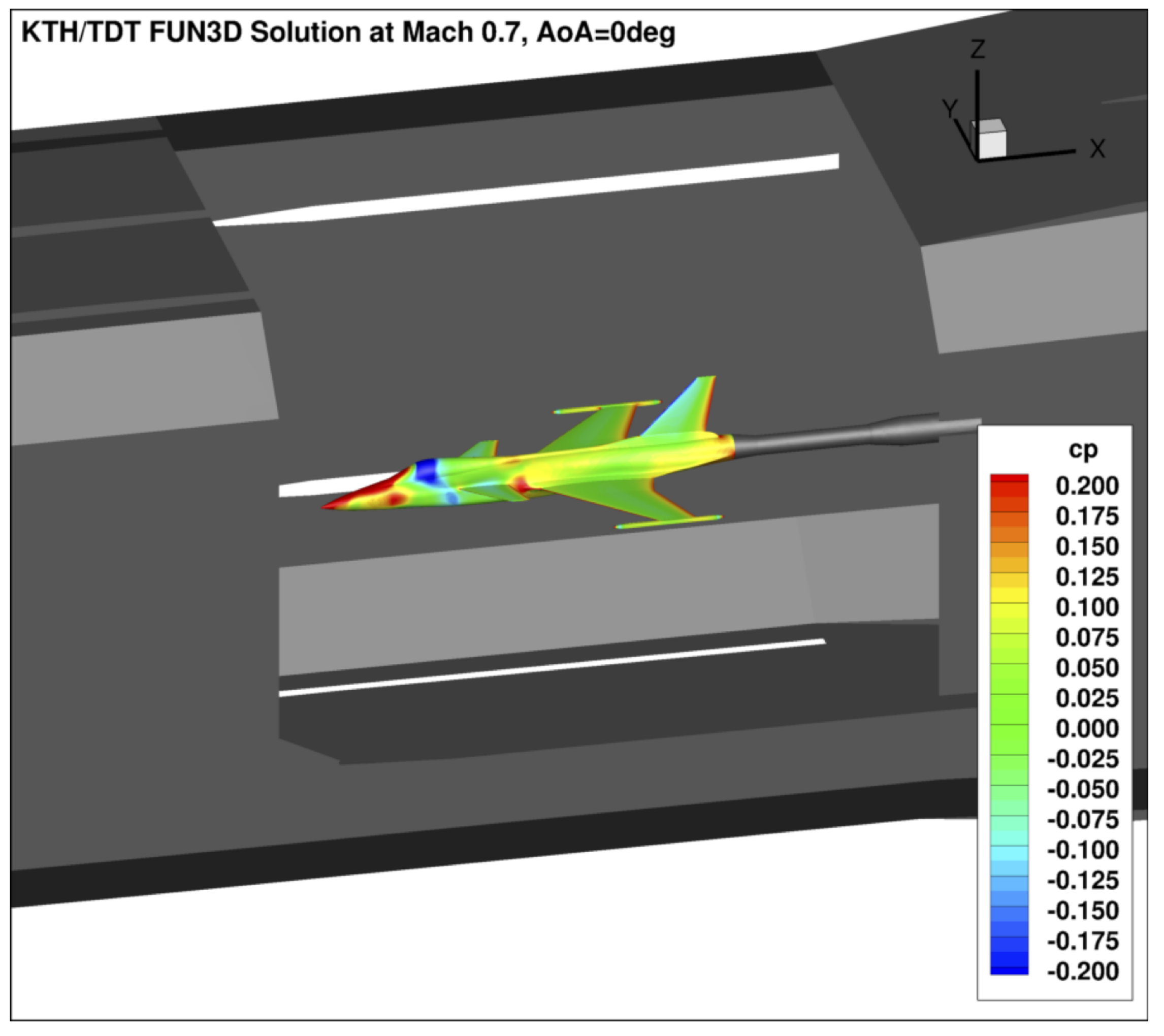
Using the AEROM software, aeroelastic root locus plots were generated for the KTH wind-tunnel model in air test medium for a free-air case and a solution accounting for the effects of the TDT test section via CFD modeling [33,34], as can be seen in Figure 12. There were three configurations tested: wing with tip stores (configuration 1), wing with tip and under-wing stores (configuration 2), and wing with tip and under-wing stores with added masses at tip stores (configuration 3). The third configuration exhibited flutter while configurations 1 and 2 did not. Presented in Figure 13 is the aeroelastic ROM root locus plot for the free-air configuration at M = 0.90. For this case, the roots clearly indicate a flutter mechanism at about 8100 N/m² (or 169 psf) via a coalescence of modes 5 and 6. Using the ROM, any dynamic pressure can be quickly evaluated to determine the aeroelastic response, consistent with the root locus plots. At this dynamic pressure, the ROM-based flutter prediction is above the experimental flutter dynamic pressure at M = 0.9. Typically, a conservative flutter result occurs when the analysis predicts a flutter condition below the experimental flutter result. This result, therefore, implies a non-conservative result, indicative of potentially significantly non-linear phenomena. All results presented are for zero structural damping. Using the ROM, the effect of structural damping can be quickly evaluated as well but is not pursued in the present discussion.

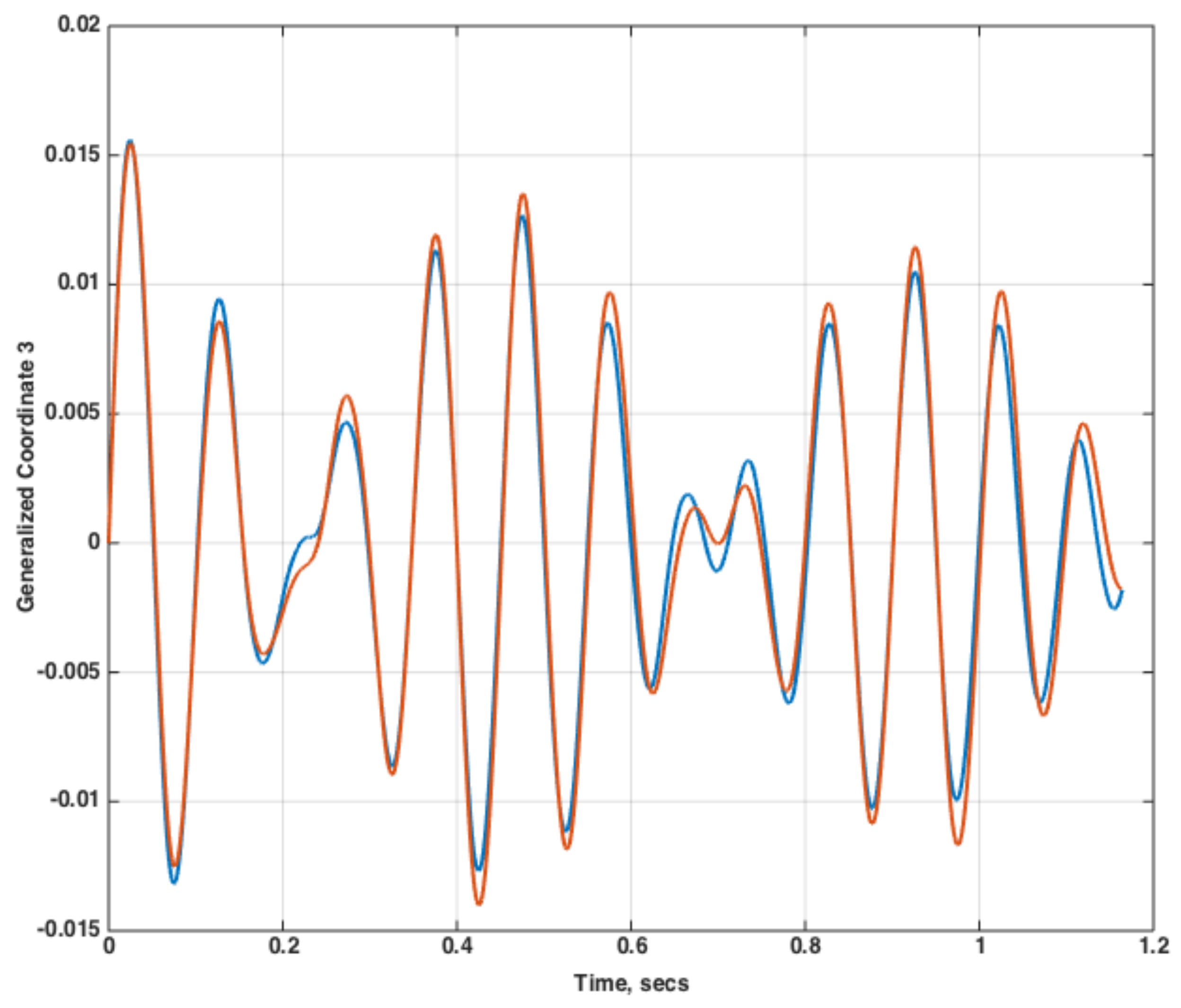
Presented in Figure 14 and Figure 15 are comparisons of the aeroelastic responses for modes 3, 4, 5, and 6 at M = 0.9 and Q = 7344 Pa for the FUN3D solution that includes the effect of the TDT and the ROM solution for the same configuration. As can be seen, the comparison is quite good with some variation in mode 6. Additional studies are currently underway to minimize these variations in order to reduce the error associated with the ROM.

For the CFD model that included the TDT, the ROM solution required two days whereas the full solution (for only one dynamic pressure) required five days. The ROM solution could, of course, then be used to rapidly compute the aeroelastic response due to any dynamic pressure.

4.3. AGARD 445.6 Wing

Aeroelastic transients for the AGARD 445.6 aeroelastic wing [35] from the FUN3D full solution and from the aeroelastic ROM, for inviscid and viscous solutions, are presented in this section. The FUN3D full solution aeroelastic transients are presented for two Mach numbers (M = 0.96, M = 1.141) at various dynamic pressures. FUN3D full and ROM aeroelastic solutions are compared at specific dynamic pressures, including root locus plots.

4.3.1. Inviscid Results

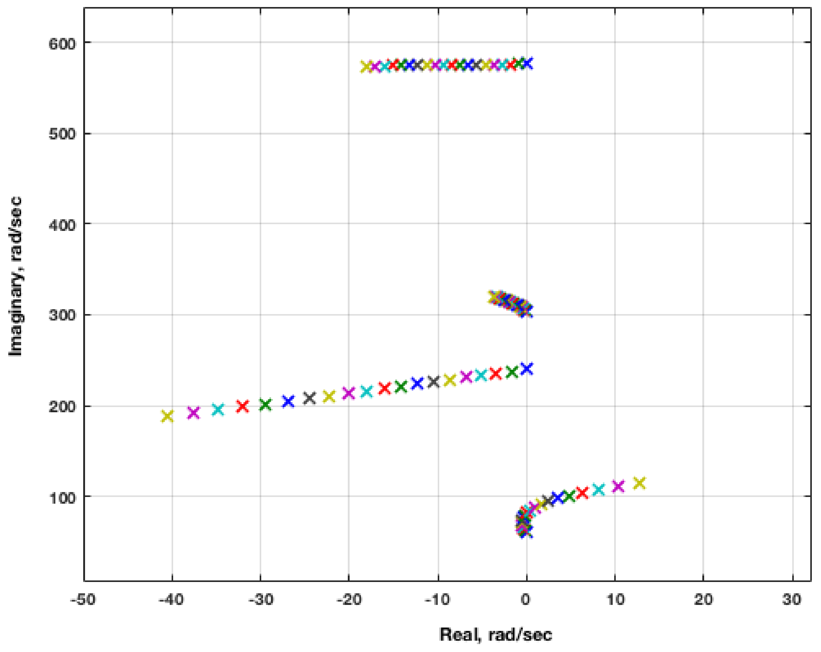
Inviscid FUN3D full and ROM solutions are presented in this section. The aeroelastic root locus plot for M = 0.96 generated using the ROM method is presented in Figure 16. In these root locus plots, dynamic pressures vary from zero to 114 psf in twenty increments. These root locus plots can be generated for any number, and any increment, of dynamic pressures rapidly. A flutter mechanism dominated by the first mode with some coupling with the second mode is indicated at this Mach number, while the third and fourth modes are stable.

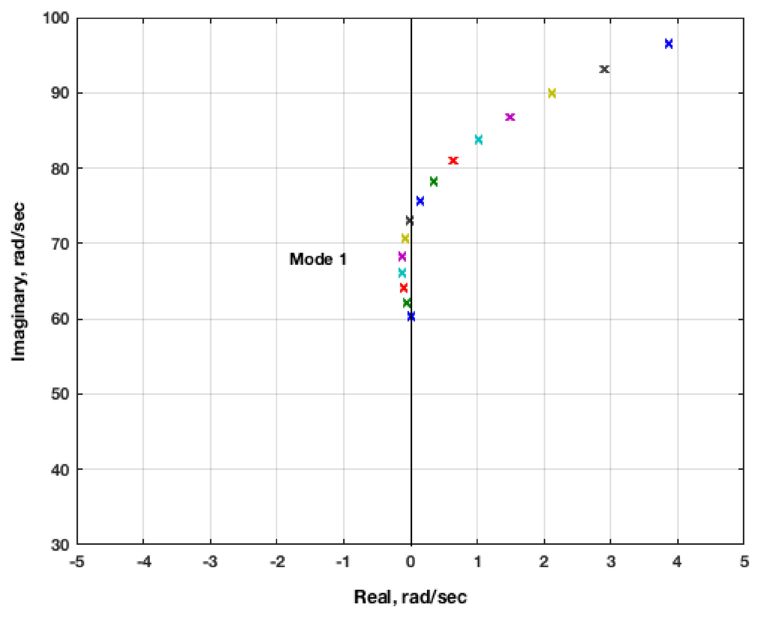
Figure 17 presents a close-up version of the root locus plot. The dynamic pressure for this root locus plot starts at 0 psf with an increment of 6 psf, resulting in a flutter dynamic pressure of approximately 30 psf, consistent with the full FUN3D solution flutter dynamic pressure [35]. The inviscid result does not compare well with the experimental flutter dynamic pressure at this Mach number. Inviscid solutions tend to have stronger shocks that are farther aft and, therefore, induce a stronger and earlier onset of flutter, so this discrepancy is not surprising. Including viscosity, the shock strength is reduced and the shock moves forward, yielding a higher flutter dynamic pressure.

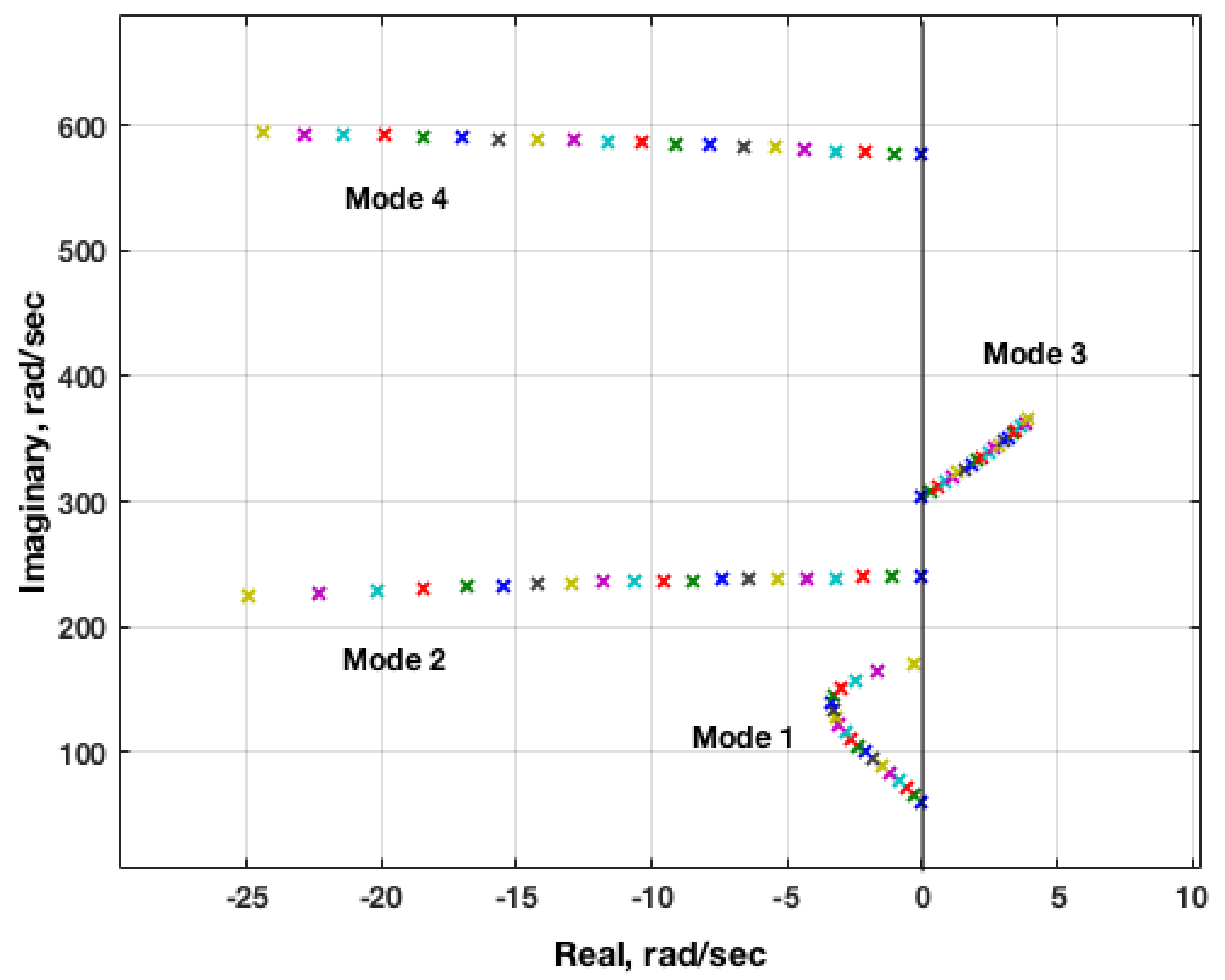
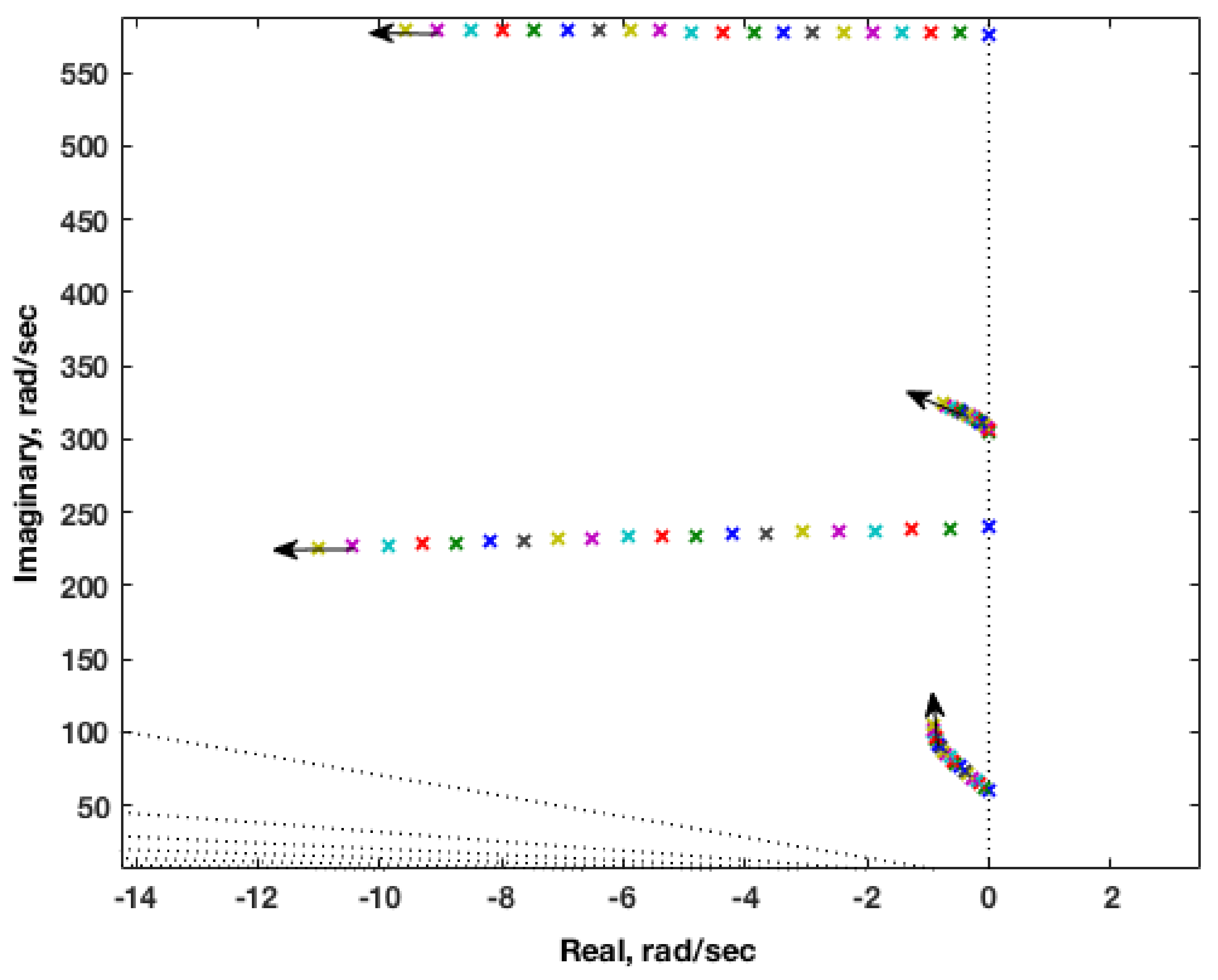
Figure 18 presents the ROM aeroelastic root locus plot for M = 1.141. There are two flutter mechanisms at this condition. The first flutter mechanism consists of a first-mode instability at a dynamic pressure of about 300 psf. The second flutter mechanism involves a third-mode instability that is always unstable. In order to validate the accuracy of this aeroelastic root locus plot, the generalized coordinates from a full FUN3D solution are analyzed.

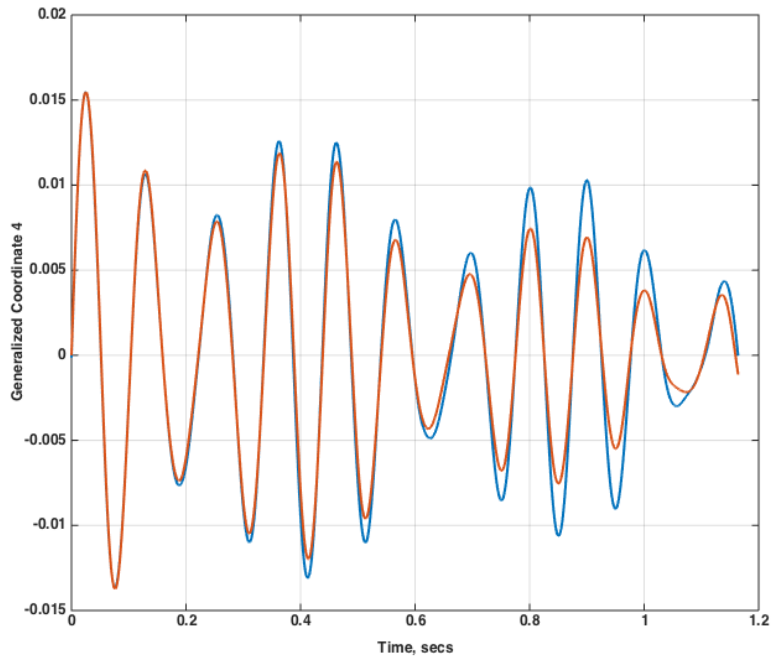
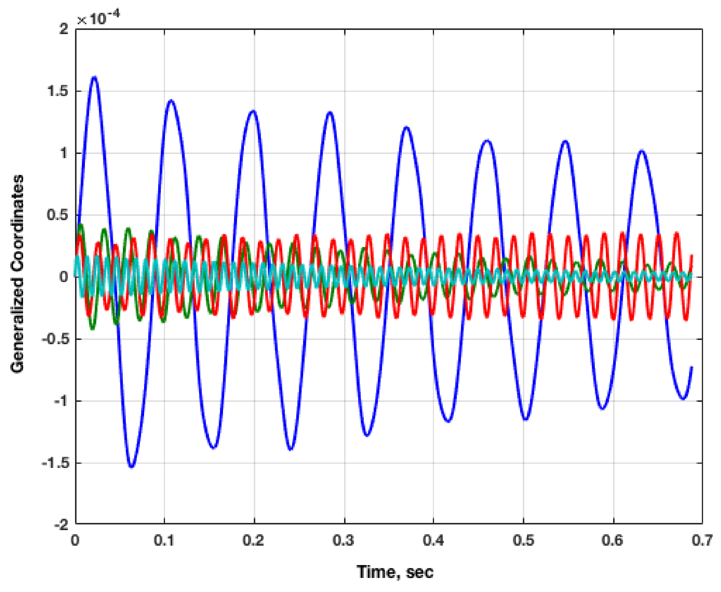
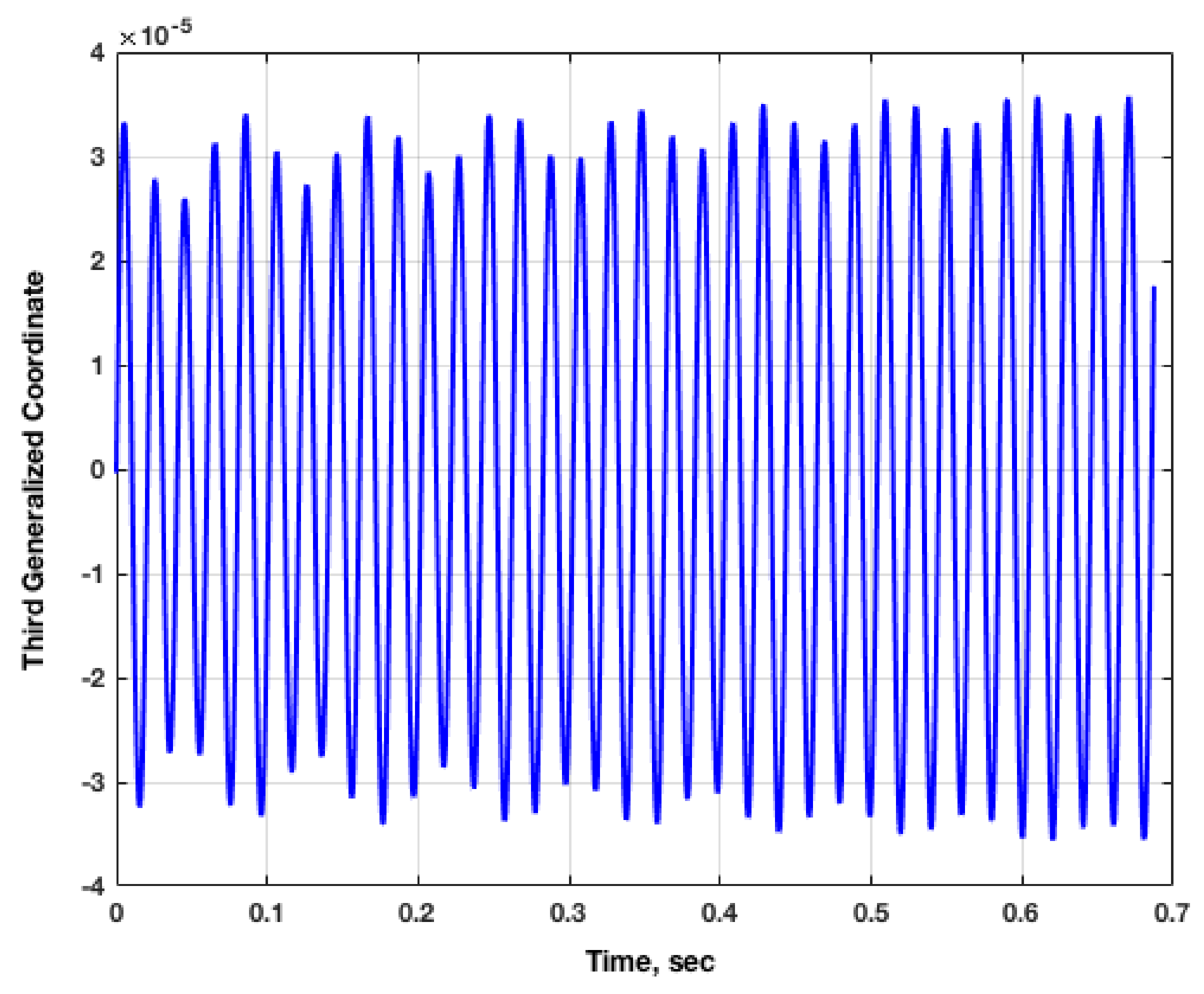
A visual examination of the aeroelastic transients for the four modes at M = 1.141 and a dynamic pressure of 30 psf, presented in Figure 19, indicate that the first mode, with the largest amplitude, is clearly stable. The stability of the other three modes is harder to discern due to smaller and similar amplitudes. Figure 20 presents the generalized coordinate response of the third mode, clearly showing that this mode becomes unstable.

Other publications on the flutter boundary of the AGARD 445.6 wing do not mention this third mode instability. It is not clear if this instability is present in all inviscid (Euler) solutions of the AGARD 445.6 wing. It is possible that the first mode instability dominated all inviscid analyses at supersonic conditions to date. If evaluation of stability was based on a visual examination of the generalized coordinates, it is understandable how the third mode instability might have been missed. Analyses performed in the early days of computational aeroelasticity would have consisted of fewer time steps (due to computational cost at the time), thereby making it difficult to visually notice the third mode instability presented in Figure 19. The authors have confirmed the existence of this third mode instability in previous solutions obtained using the NASA Langley CFL3D code as well.

4.3.2. Viscous Results

Viscous FUN3D full and ROM solutions are presented at M = 1.141 in this section. The results for FUN3D full and ROM viscous solutions at subsonic Mach numbers agree well with each other and with experiment and are not presented here.

The root locus plot generated using the FUN3D ROM viscous solution at M = 1.141, in dynamic pressure increments of 6 psf to 114 psf, is presented as Figure 21. It is clear that the inclusion of viscous effects has stabilized the third mode instability noticed in the inviscid solution.

A fundamental difference exists between a root locus plot and the post-processed analysis of generalized coordinates over a short period of time. By definition, a root locus plot reveals the roots of a system as time approaches infinity. The analysis of the initial transient response of a generalized coordinate over a short period of time, on the other hand, can be deceiving as the response can change if the response was viewed (or analyzed) over a longer period of time. This property of root locus plots is critical for the accurate evaluation of aeroelastic stability.

5. Conclusions

The origin, implementation, and applications of AEROM, the patented NASA reduced-order modeling software, have been presented. Recent applications of the software to analyze complex configurations, including computation of the aeroelastic responses of the Lockheed-Martin low-boom N+2 configuration, the KTH (Royal Institute of Technology, Stockholm, Sweden) generic fighter wind-tunnel model, and the AGARD 445.6 wing were presented. The results presented here demonstrate the computational efficiency and analytical capability of the AEROM software.

References

- Adams, W.M.; Hoadley, S.T. ISAC: A Tool for Aeroservoelastic Modeling and Analysis. In Proceedings of the 34th AIAA/ASME/ASCE/AHS/ASC Structures, Structural Dynamics, and Materials Conference, La Jolla, CA, USA, 19–22 April 1993. AIAA-1993-1421. [Google Scholar]
- Silva, W.A. Simultaneous Excitation of Multiple-Input/Multiple-Output CFD-Based Unsteady Aerodynamic Systems. J. Aircr. 2008, 45, 1267–1274. [Google Scholar] [CrossRef]
- Silva, W.A.; Vatsa, V.N.; Biedron, R.T. Development of Unsteady Aerodynamic and Aeroelastic Reduced-Order Models Using the FUN3D Code. Presented at the International Forum on Aeroelasticity and Structural Dynamics, Seattle, WA, USA, 21–25 June 2009. IFASD Paper No. 2009-30. [Google Scholar]
- Silva, W.A.; Vatsa, V.N.; Biedron, R.T. Reduced-Order Models for the Aeroelastic Analyses of the Ares Vehicles. Presented at the 28th AIAA Applied Aerodynamics Conference, Chicago, IL, USA, 28 June–1 July 2010. AIAA Paper No. 2010-4375. [Google Scholar]
- Silva, W.A. Discrete-Time Linear and Nonlinear Aerodynamic Impulse Responses for Efficient CFD Analyses. Ph.D. Thesis, College of William & Mary, Williamsburg, VA, USA, December 1997. [Google Scholar]
- Silva, W.A. Identification of Linear and Nonlinear Aerodynamic Impulse Responses Using Digital Filter Techniques. In Proceedings of the Atomospheric Flight Mechanics, New Orleans, LA, USA, 11–13 August 1997. AIAA Paper 97-3712. [Google Scholar]
- Silva, W.A. Reduced-Order Models Based on Linear and Nonlinear Aerodynamic Impulse Responses. In Proceedings of the CEAS/AIAA/ICASE/NASA Langley International Forum on Aeroelasticity and Structural Dynamics, Williamsburg, VA, USA, 22–25 June 1999; pp. 369–379. [Google Scholar]
- Juang, J.-N.; Pappa, R.S. An Eigensystem Realization Algorithm for Modal Parameter Identification and Model Reduction. J. Guidance Control Dyn. 1985, 8, 620–627. [Google Scholar] [CrossRef]
- Juang, J.-N. Applied System Identification; Prentice-Hall PTR: Upper Saddle River, NJ, USA, 1994. [Google Scholar]
- Silva, W.A.; Raveh, D.E. Development of Unsteady Aerodynamic State-Space Models from CFD-Based Pulse Responses. Presented at the 42nd Structures, Structural Dynamics, and Materials Conference, Seattle, WA, USA, 16–19 April 2001. AIAA Paper No. 2001-1213. [Google Scholar]
- Gaitonde, A.L.; Jones, D.P. Study of Linear Response Identification Techniques and Reduced-Order Model Generation for a 2D CFD Scheme. J. Numer. Methods Fluids 2006, 52, 1367–1402. [Google Scholar] [CrossRef]
- Gaitonde, A.L.; Jones, D.P. Calculations with ERA Based Reduced-Order Aerodynamic Models. In Proceedings of the 24th Applied Aerodynamics Conference, San Francisco, CA, USA, 5–8 June 2006. [Google Scholar]
- Griffiths, L.; Jones, D.P.; Friswell, M.I. Model Updating of Dynamically Time Linear Reduced-Order Models. In Proceedings of the International Forum on Aeroelasticity and Structural Dynamics, Paris, France, 27–30 June 2011. [Google Scholar]
- Fleischer, D.; Breitsamter, C. Efficient Computation of Unsteady Aerodynamic Loads Using Computational Fluid Dynamics Linearized Methods. J. Aircr. 2013, 50, 425–440. [Google Scholar] [CrossRef]
- Xiaoyan, L.; Zhigang, W.; Chao, Y. Aerodynamic Reduced-Order Models Based on Observer Techniques. In Proceedings of the 51st AIAA/ASME/ASCE/AHS/ASC Structures, Structural Dynamics, and Materials Conference, Orlando, FL, USA, 12–15 April 2010. [Google Scholar]
- Song, H.; Qian, J.; Wang, Y.; Pant, K.; Chin, A.W.; Brenner, M.J. Development of Aeroelastic and Aeroservoelastic Reduced-Order Models for Active Structural Control. In Proceedings of the 56th AIAA/ASCE/AHS/ASC Structures, Structural Dynamics, and Materials Conference, Kissimmee, FL, USA, 5–9 January 2015. [Google Scholar]
- Ma, Z.; Ahuja, S.; Rowley, C.W. Reduced-Order Models for Control of Fluid Using the Eigensystem Realization Algorithm. Theor. Comput. Fluid Dyn. 2011, 25, 233–247. [Google Scholar] [CrossRef]
- Krist, S.L.; Biedron, R.T.; Rumsey, C.L. CFL3D User’s Manual Version 5.0; Technical Report; NASA Langley Research Center: Hampton, VA, USA, 1997.
- Silva, W.A.; Bartels, R.E. Development of Reduced-Order Models for Aeroelastic Analysis and Flutter Prediction Using the CFL3Dv6.0 Code. J. Fluids Struct. 2004, 19, 729–745. [Google Scholar] [CrossRef]
- Kim, T.; Hong, M.; Bhatia, K.G.; SenGupta, G. Aeroelastic Model Reduction for Affordable Computational Fluid Dynamics-Based Flutter Analysis. AIAA J. 2005, 43, 2487–2495. [Google Scholar] [CrossRef]
- Silva, W.A. Recent Enhancements to the Development of CFD-Based Aeroelastic Reduced Order Models. In Proceedings of the 48th AIAA/ASME/ASCE/AHS/ASC Structures, Structural Dynamics, and Materials Conference, Honolulu, HI, USA, 23–26 April 2007. AIAA Paper No. 2007-2051. [Google Scholar]
- Anderson, W.K. Bonhaus, D.L. An Implicit Upwind Algorithm for Computing Turbulent Flows on Unstructured Grids. Comput. Fluids 1994, 23, 1–21. [Google Scholar] [CrossRef]
- NASA LaRC. FUN3D Manual, v12.9; NASA LaRC: Hampton, VA, USA, 2015. Available online: http://fun3d.larc.nasa.gov (accessed on 21 September 2015).
- Biedron, R.T.; Vatsa, V.N.; Atkins, H.L. Simulation of Unsteady Flows Using an Unstructured Navier-Stokes Solver on Moving and Stationary Grids. In Proceedings of the 23rd AIAA Applied Aerodynamics Conference, Toronto, ON, Canada, 6–9 June 2005. AIAA Paper 2005-5093. [Google Scholar]
- Biedron, R.T.; Thomas, J.L. Recent Enhancements to the FUN3D Flow Solver for Moving-Mesh Applications. In Proceedings of the 47th AIAA Aerospace Sciences Meeting Including The New Horizons Forum and Aerospace Exposition, Orlando, FL, USA, 5–8 January 2009; AIAA Paper 2009-1360. Available online: https://arc.aiaa.org/doi/abs/10.2514/6.2009-1360 (accessed on 10 April 2009).
- Juang, J.-N.; Phan, M.; Horta, L.G.; Longman, R.W. Identification of Observer/Kalman Filter Markov Parameters: Theory and Experiments. J. Guid. Control Dyn. 1993, 16, 320–329. [Google Scholar] [CrossRef]
- Eykhoff, P. System Identification: Parameter and State Identification; Wiley Publishers: Hoboken, NJ, USA, 1974. [Google Scholar]
- Ljung, L. System Identification: Theory for the User; Prentice-Hall Publishers: Upper Saddle River, NJ, USA, 1999. [Google Scholar]
- Zhu, Y. Multivariable System Identification for Process Control; Pergamon Publishers: Oxford, UK, 2001. [Google Scholar]
- Pacheco, R.P.; Steffen, V., Jr. Using Orthogonal Functions for Identification and Sensitivity Analysis of Mechanical Systems. J. Vib. Control 2002, 8, 993–1021. [Google Scholar] [CrossRef]
- Raveh, D.E. Identification of Computational-Fluid-Dynamic Based Unsteady Aerodynamic Models for Aeroelastic Analysis. J. Aircr. 2004, 41, 620–632. [Google Scholar] [CrossRef]
- Silva, W.A.; Ringertz, U.; Stenfelt, G.; Eller, D.; Keller, D.F.; Chwalowski, P. Status of the KTH-NASA Wind-Tunnel Test for Acquisition of Transonic Nonlinear Aeroelastic Data. In Proceedings of the 15th Dynamics Specialists Conference, AIAA SciTech Forum, San Diego, CA, USA, 4–8 January 2016. No. AIAA 2016-2050. [Google Scholar]
- Silva, W.A.; Chwalowski, P.; Wieseman, C.D.; Keller, D.F.; Eller, D.; Ringertz, U. Computational and Experimental Results for the KTH-NASA Wind-Tunnel Model Used for Acquistion of Transonic Nonlinear Aeroelastic Data. In Proceedings of the International Forum on Aeroelasticity and Structural Dynamics, Como, Italy, 26–28 June 2017. [Google Scholar]
- Chwalowski, P.; Silva, W.A.; Wieseman, C.D.; Heeg, J. CFD Model of the Transonic Dynamics Tunnel with Applications. In Proceedings of the International Forum on Aeroelasticity and Structural Dynamics, Como, Italy, 26–28 June 2017. [Google Scholar]
- Silva, W.A.; Chwalowski, P.; Perry, B. Evaluation of Linear, Inviscid, Viscous, and Reduced-Order Modeling Aeroelastic Solutions of the AGARD 445.6 Wing Using Root Locus Analysis. Int. J. Comput. Fluid Dyn. 2014, 28, 122–139. [Google Scholar] [CrossRef]
Figure 1.
Walsh functions.
Figure 2.
Improved process for generation of an unsteady aerodynamic reduced-order modeling (ROM) (Steps 1–4).
Figure 3.
Process for generation of a structural dynamic state-space ROM.
Figure 4.
Process for generation of an aeroelastic simulation ROM consisting of an unsteady aerodynamic ROM and a structural dynamic state-space ROM.
Figure 5.
Error defined as difference between the FUN3D solution and the unsteady aerodynamic ROM solution due to input of orthogonal functions.
Figure 6.
Artist’s concept of the Lockheed-Martin N+2 configuration.
Figure 7.
Comparison of full FUN3D aeroelastic response and ROM aeroelastic response for the first mode of the N+2 configuration at M = 1.7 and a dynamic pressure of 2.149 psi.
Figure 8.
Comparison of full FUN3D aeroelastic response and ROM aeroelastic response for the second mode of the N+2 configuration at M = 1.7 and a dynamic pressure of 2.149 psi.
Figure 9.
Aeroelastic root locus plot for the low-boom N+2 configuration at M = 1.7 with each colored marker indicating an increment of 2 psi in dynamic pressure for a given mode.
Figure 10.
The generic fighter aeroelastic wind-tunnel model tested in summer of 2016.
Figure 11.
The generic fighter aeroelastic wind-tunnel model installed in the Transonic Dynamics Tunnel (TDT).
Figure 12.
Pressure distributions at M = 0.7, AoA = 0 degrees on the KTH wind-tunnel model, as simulated inside the TDT using FUN3D code.
Figure 13.
Root locus plot generated from ROM model indicating an aeroelastic instability at M = 0.90 in air test medium for the third configuration with each colored marker indicating an increment of 450 N/m2 in dynamic pressure for a given mode.
Figure 14.
Aeroelastic response in mode 3 for the FUN3D (blue) and ROM (orange) solutions for the configuration including the Transonic Dynamics Tunnel (TDT).
Figure 15.
Aeroelastic response in mode 4 for the FUN3D (blue) and ROM (orange) solutions for the configuration including the TDT.
Figure 16.
ROM aeroelastic root locus plot for M = 0.96, inviscid solution.
Figure 17.
Detailed view of ROM aeroelastic root locus plot for M = 0.96, inviscid solution.
Figure 18.
ROM aeroelastic root locus plot for M = 1.141, inviscid solution.
Figure 19.
FUN3D full solution generalized coordinates at M = 1.141, Q = 30 psf, inviscid solution. Mode 1 = blue, Mode 2 = green, Mode 3 = red, Mode 4 = cyan.
Figure 20.
FUN3D full solution third generalized coordinate at M = 1.141, Q = 30 psf, inviscid solution.
Figure 21.
Viscous ROM root locus plot at M = 1.141.
© 2018 by the author. Licensee MDPI, Basel, Switzerland. This article is an open access article distributed under the terms and conditions of the Creative Commons Attribution (CC BY) license (http://creativecommons.org/licenses/by/4.0/).
Share and Cite
MDPI and ACS Style
Silva, W.A. AEROM: NASA’s Unsteady Aerodynamic and Aeroelastic Reduced-Order Modeling Software. Aerospace 2018, 5, 41. https://doi.org/10.3390/aerospace5020041
AMA Style
Silva WA. AEROM: NASA’s Unsteady Aerodynamic and Aeroelastic Reduced-Order Modeling Software. Aerospace. 2018; 5(2):41. https://doi.org/10.3390/aerospace5020041
Chicago/Turabian StyleSilva, Walter A. 2018. "AEROM: NASA’s Unsteady Aerodynamic and Aeroelastic Reduced-Order Modeling Software" Aerospace 5, no. 2: 41. https://doi.org/10.3390/aerospace5020041
Note that from the first issue of 2016, this journal uses article numbers instead of page numbers. See further details here.