Flight Load Assessment for Light Aircraft Landing Trajectories in Windy Atmosphere and Near Wind Farms
by
 , , , and
Carmine Varriale
1 ,
,
Agostino De Marco
1 ,
,
Elia Daniele
2,*,
Jonas Schmidt
2 and
Bernhard Stoevesandt
2 1
Department of Industrial Engineering, University of Naples Federico II, Via Claudio 21, 80125 Naples, Italy
2
Fraunhofer Institute for Wind Energy Systems, IWES, Küpkersweg 70, 26129 Oldenburg, Germany
*
Author to whom correspondence should be addressed.
Aerospace 2018, 5(2), 42; https://doi.org/10.3390/aerospace5020042
Submission received: 16 February 2018
/
Revised: 4 April 2018
/
Accepted: 5 April 2018
/
Published: 10 April 2018
(This article belongs to the Special Issue Feature Papers in Aerospace)
Abstract
:This work focuses on the wake encounter problem occurring when a light, or very light, aircraft flies through or nearby a wind turbine wake. The dependency of the aircraft normal load factor on the distance from the turbine rotor in various flight and environmental conditions is quantified. For this research, a framework of software applications has been developed for generating and controlling a population of flight simulation scenarios in presence of assigned wind and turbulence fields. The JSBSim flight dynamics model makes use of several autopilot systems for simulating a realistic pilot behavior during navigation. The wind distribution, calculated with OpenFOAM, is a separate input for the dynamic model and is considered frozen during each flight simulation. The aircraft normal load factor during wake encounters is monitored at different distances from the rotor, aircraft speeds, rates of descent and crossing angles. Based on these figures, some preliminary guidelines and recommendations on safe encounter distances are provided for general aviation aircraft, with considerations on pilot comfort and flight safety. These are needed, for instance, when an accident risk assessment study is required for flight in proximity of aeolic parks. A link to the GitHub code repository is provided.
1. Introduction
1.1. Wind Turbines Impact on Aviation
In the last fifteen years, the wind power industry has constantly gained a relentless and rapid market growth all over the world [1]. As a consequence of the spread of wind farms operation sites, it is easy to understand how, to this day, the most easily accessible locations have already been used up: these are the ones located at sufficient distance from communities, with no environmental or aeronautical constraints, and with good access to the grid network. Attention has therefore recently turned to the more challenging sites and more and more issues have started to arise for the aviation sector. During 2015 in Germany, about 4100 of planned wind turbine projects were stopped for incompatibility with existing aviation and radar facilities [2]. The specific situation we have investigated in this work is represented by general aviation users operating near unlicensed aerodromes, focusing the attention on light and ultra-light fixed-wing aircraft.
A classification of the different types of impact that wind turbines may have on the aviation sector should consider several issues [3]. Firstly, a wind turbine may provide a physical obstruction to the continued safety of flight. The introduction of such obstacles reduces the area available to pilots during low-altitude flying operations, and these circumstances also have strong financial impact on aerodromes used mostly for training and leisure purposes. Secondly, turbulence effects are noticeable up to many diameters downstream of the wind turbine. When a pilot approaches a non-towered airport, he is supposed to follow a conventional traffic pattern ending with the most delicate landing maneuver [4]. In this phase, the aircraft is flying close to the stall speed, and likely in more or less intense crosswind conditions depending on the surroundings and the environment. Though wind shear is generally short lived, it is one of the greatest hazards to aircraft at low altitude. Terrain morphology, constructed obstructions, thermals, temperature inversions are all ordinary causes of wind shears, and it is clear that the existence of a wind farm in proximity of an aerodrome can definitely be a complication. Lastly, rotating blades are a source of clutter for radio and radar equipment [5,6,7].
According to the most recent statistics on aviation accidents for fixed-wing non-commercial aircraft, both the number of total injuries/fatalities and of aircraft incidents in the last 10 years have decreased. Nevertheless, the primary causes of accidents are clearly identified to be, in order of importance, the aircraft being upset in flight (47%), terrain conflict (23%) and obstacle interference (9%) [8]. For general aviation non-commercial flight below a maximum take-off mass of 5700 kg in 2016, the most numerous accidents occurred during pleasure flights (, 62%) while the second most numerous occurred during instructional/training flights (, 9%); 49% of accidents, ultimately, occurred during approach or landing. This data is also perfectly in line with the statistics from the previous 10 years (2006–2015) [8]. From January 2006 to December 2016, 248 accidents of private aircraft carrying more than six people led to the retirement of the aircraft from service. Of these, 105 (42%) happened during approach or landing, and 10 (4%) are due to weather conditions [9]. Although the ultimate cause for these accidents is hard to trace, the top human-factor safety issues are identified to be related to deficit in situational awareness, lack of flight planning information and lack of experience, training and competence of the individuals (especially for private pilots). All these factors may concur to loss of control of the aircraft during complex flight scenarios [8].
Whilst the effect of aircraft induced turbulence on other aircraft is well understood, as well as that of wind turbines on other wind turbines, the potential effects of wind turbine-induced turbulence on aircraft have gathered only limited attention from a few researchers [10,11,12,13] in general terms to date. All instances must be considered on their own merits, depending on the aircraft category, flight operations, turbine size, and prevailing wind conditions, but it is clear how paramount it is to continue scientific investigation in this direction. This paper addresses the problem of controllability of a light aircraft during a wake encounter flight by prescribing a trajectory for a simple autopilot system to follow. The effect of the necessary control actions on the aircraft are observed through the analysis of the aircraft load factor , which synthesizes considerations on both structural safety and comfort on board.
1.2. Aircraft Load Factor and V-n Diagram
According to existing regulations for light and very light aircraft, the capacity an aircraft has to structurally withstand forces due to either maneuvers or gusts is quantified by the maximum and minimum load factor it is designed for. The normal load factor is defined in magnitude and sign as , and therefore represents a global normalized measure of the acceleration an aircraft is subjected to, due to external loads along its vertical body axis. Human beings as well as airplane structures have a limited ability to withstand load factors significantly diverging from the nominal condition of . This is why aviation authorities specify the load factor limits within which different classes of aircraft are required to operate without damage, i.e., without the possibility of external forces to exceed the structural strength of the airplane components. For very light aircraft, regulations prescribe that the airplane must be able to sustain a positive maneuvering load factor of up to a minimum of , and a negative maneuvering load factor of down to a minimum of . The limit gust load factor has to be considered as linearly varying with aircraft airspeed, starting from a value of 1 at zero aircraft speed. A reference gust speed ( ·, i.e., 50 ·) is given for aircraft cruise speed , and the limit gust load factor at can then be calculated by using Equation (1):
Alternatively, other methods can be implemented, but the “1-cos” gust profile as in Equation (2) has to be adopted for the aircraft certification [14]. For this work, also a second approach was taken by integrating Equation (3) in the unknown instantaneous vertical speed . This is the equation for the point-mass aircraft vertical dynamics after an encounter with a given gust profile , and results in the time history of during the gust encounter. The outcome of the two methods from Equations (1) and (3) is reported in Section 3.2:
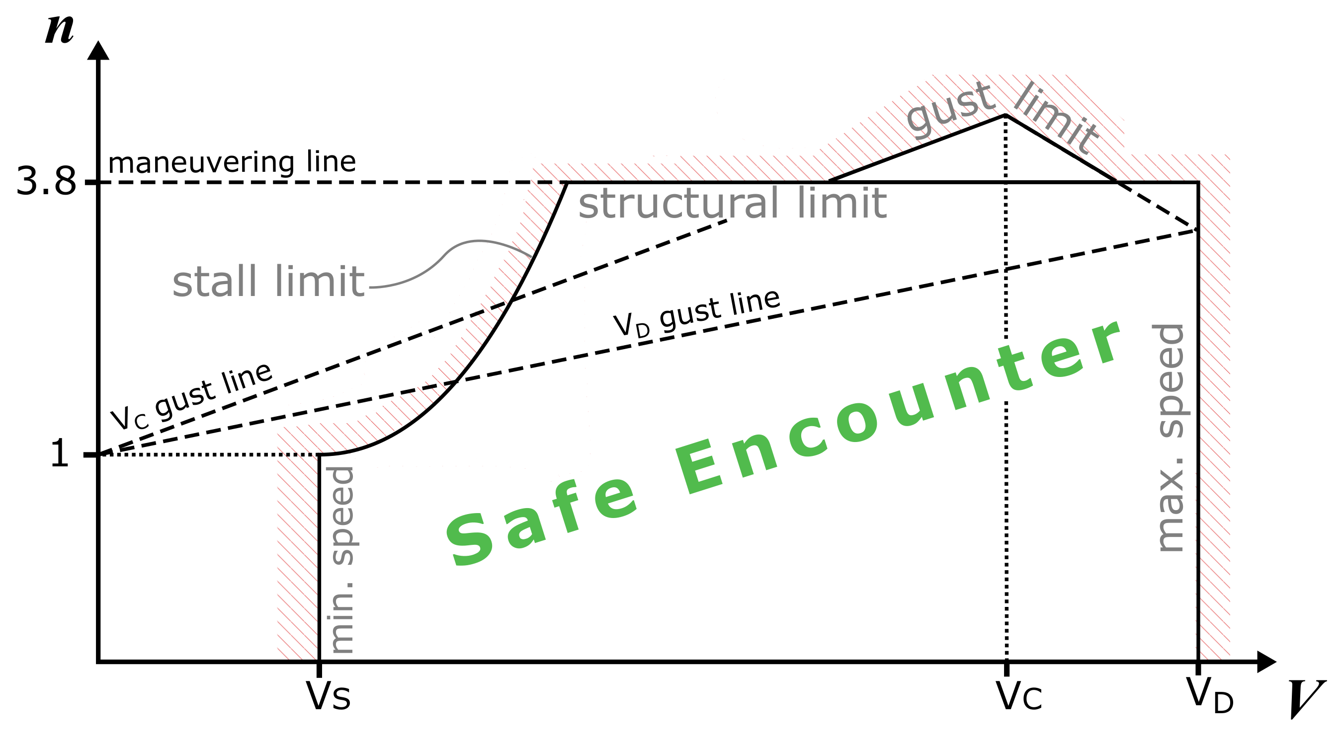
Once the V-n diagram for the given aircraft is drawn as reported qualitatively in Figure 1, the limit values for the load factor due to both maneuvering and gusts are identified. It is possible that the gust limit falls either within or outside of the maneuvering limit, depending on the specific case.
For speeds close to the stall speed , the V-n diagram also shows that high loads will result in the aircraft stalling before suffering structural damage: this is therefore an aerodynamic limit that results in the pilot losing control of the aircraft, without compromising its immediate safety. The stall limit curve has a parabolic shape given by the following Equation (4), which expresses the vertical equilibrium in maneuvering condition:
At stall speed , the maximum allowable load factor is obtained in level flight at the maximum lift coefficient , i.e., at . This means that, in stalling conditions, the aircraft is not able to do any maneuver that increases its normal load factor without stalling. For , the maximum load factor is also obtained at the maximum lift coefficient, but grows with speed up to the limit imposed by regulations for structural safety. To sum up, the turbine wake encounter can be considered safe if the load factor experienced during the flight falls within the largest of all these design boundaries [14].
1.3. Modelling
A thorough discussion of wind turbine wakes lies outside the scope of this work. Nevertheless, some useful observations for the comprehension of the proposed approach are provided in the following. The main focus for the wake encounter object of this study lies in the near wake region, since the restrictions on wind farm layouts are mainly driven by reduced allowable installation space sharing borders with aerodromes. In the near wake region, it is still possible to identify the trailed vortex structures released by the root-hub and tip regions, and convected downstream with the mean wind velocity behind the rotor plane. This is particularly true if the effects of turbulence inflow, complex terrain and boundary layer are neglected, as in this study. Computational Fluid Dynamics (CFD) methods have been recently used to study wake development and breakdown [15,16]. The Actuator Disk Model (ADM) and the Actuator Line Model (ALM) are two of the most used methods to simulate the turbine rotor and obtain a satisfying degree of fidelity for the flow stream downwind of it [17,18,19,20].
Interfacing the former types of simulation with a flight dynamics model involves combining two very different branches of physics, and may be carried out successfully with increasing levels of approximation. The wind velocity distribution may or may not be evolving in time together with the aircraft motion, and it could be obtained by analytical models or by simulation. The instantaneous wind velocity vector could be integrated in the aircraft aerodynamic model through a single-point (e.g., only center of gravity) or a multi-point interpolation.
The most common practice for such wake encounter studies is using CFD techniques, as well as experimental campaigns in wind tunnels, exclusively for tuning and validation of more simple, steady analytical turbine wake models. Only these latter ones are ultimately implemented in the flight dynamics counterpart of the wake encounter simulation, causing velocity fluctuations and other turbulent and unsteady effects not to be included in the study of the whole phenomenon. Several of them are available in literature, with different levels of complexity [21,22,23,24,25].
From a more operational perspective, test pilots can be able, by means of trials, to establish quantitatively the severity of the wake encounter, thus providing useful information to the civil aviation authorities [26]. Subjective feedback may be provided in the form of a short questionnaire, in order to define a measuring scale for the wake encounter effect on the aircraft state and the pilot’s ability to recover [13].
1.4. The Importance of Aeronautical Studies
Pilots’ personal and subjective evaluations cannot substitute aeronautic regulations that are defined by authorities on the basis of some historical evidence and/or engineering study. As an example, in the particular case of airborne collision with an on-ground obstacle, historical data series have been used to define clearance rules above aerodromes: a series of Obstacle Limitation Surfaces (OLS) are established, in order to define the limits beyond which objects must not project into the airspace. When an obstacle is designed in such a way that it intrudes, even slightly, one of the prescribed volumes, the manufacturer is required to provide an aeronautical study to prove that the obstacle does not modify the established safety level and the regularity of flight operations. At the present time, there are no further guidelines provided by regulations on how this task has to be carried out.
In the particular case of [27], the aeronautical study took advantage of advanced flight dynamics simulation techniques, with the open-source software JSBSim. Having established a reference flight situation, either a deterministic or a Montecarlo analysis can be carried out to explore the space of critical events, and consequent plausible pilot reactions to them. In the simplest case, one representative airplane model can be chosen, namely a single propeller general aviation aircraft. If a suitable subset of fatal events is determined, this can be used to support the estimation of collision risk on the basis of the obtained trajectories data.
In a similar way, it is envisioned that the aeronautical study underlying the present article will support the estimation of controllability, safety and comfort during a wind turbine wake encounter by a light aircraft.
1.5. Present Work and Structure of the Article
The present article proposes a further understanding of the aircraft-turbine wake encounter problem by quantifying the dependency of the aircraft normal load factor on the distance from the turbine rotor in various flight and environmental conditions. The work has taken full advantage of state-of-the-art open-source software for producing realistic fluid dynamics and piloted aircraft dynamics simulations. These are directly interfaced through a neutral server platform, developed just for this purpose. This framework was exploited to test different CFD models for the generation of wind turbine wakes, and make some considerations on their suitability to be integrated in a flight dynamics model, as far as a wake encounter is concerned.
The goal is to provide guidelines and recommendations on safe encounter distances for general aviation users and to improve results from a previous risk assessment study. The latter featured canonical regulation prescriptions, i.e., a point-mass aircraft model subject to a cosine gust profile in the longitudinal plane [23,24,25].
This manuscript is organized as follows: in Section 2, the proposed methodology is described. Section 3 presents the simulation scenarios that were arranged to perform the risk assessment study, with explanations on the methodology and motivation of the most relevant choices. Results are presented in a synthetic yet systematic way, and finally, in Section 4, some guidelines on a recommended pilot behavior are inferred, as they are arising from the analysis of the results.
2. Methodology
In order to simulate the aircraft-turbine wake encounter problem, the authors have used and further developed three distinct, yet interconnected, computational cores and the data management infrastructure of the project. JSBSim [28] is the dedicated flight dynamics model and simulator, while OpenFOAM [29] is the chosen toolbox for CFD simulations. In order to interface these two applications, a neutral intermediary platform has been developed from scratch: the Wind Reconstruction Server (WiReS) application. Finally, data pre- and post-processing, and simulations set-up was handled with a set of custom Python classes and implemented in a collection of progressive Jupyter Notebooks [30]. This research has been carried out using exclusively open-source software, having this philosophy unquestionable benefits in terms of productivity, as overcoming any possible proprietary software limitations and exploiting custom functionalities for specific advanced tasks. All code used and developed for this work is currently hosted on GitHub [31].
2.1. Automatic Navigation in JSBSim
A set of simple autopilot systems has been developed with the idea of simulating realistic human pilot behavior. The aim is to attain a certain specified aircraft state, such as wings level or a heading or an altitude, and hold it for a required period of time. The implemented control architecture features a series of independent, single-input-single-output (SISO), proportional-integral-derivative (PID) controllers. In our case, the control signal is an action on the aircraft control surfaces that is superimposed to the trim command actions. Each of the auto-pilot systems was tuned in order to achieve the desired response in a prescribed maneuver, i.e., few or none oscillations in the 6-degree of freedom (DOF) dynamic response and no residual error in the steady state. The tuning procedure is carried out with a campaign of trial and error test-flight simulations and supported by the Ziegler–Nichols heuristic method for PID controllers [32].
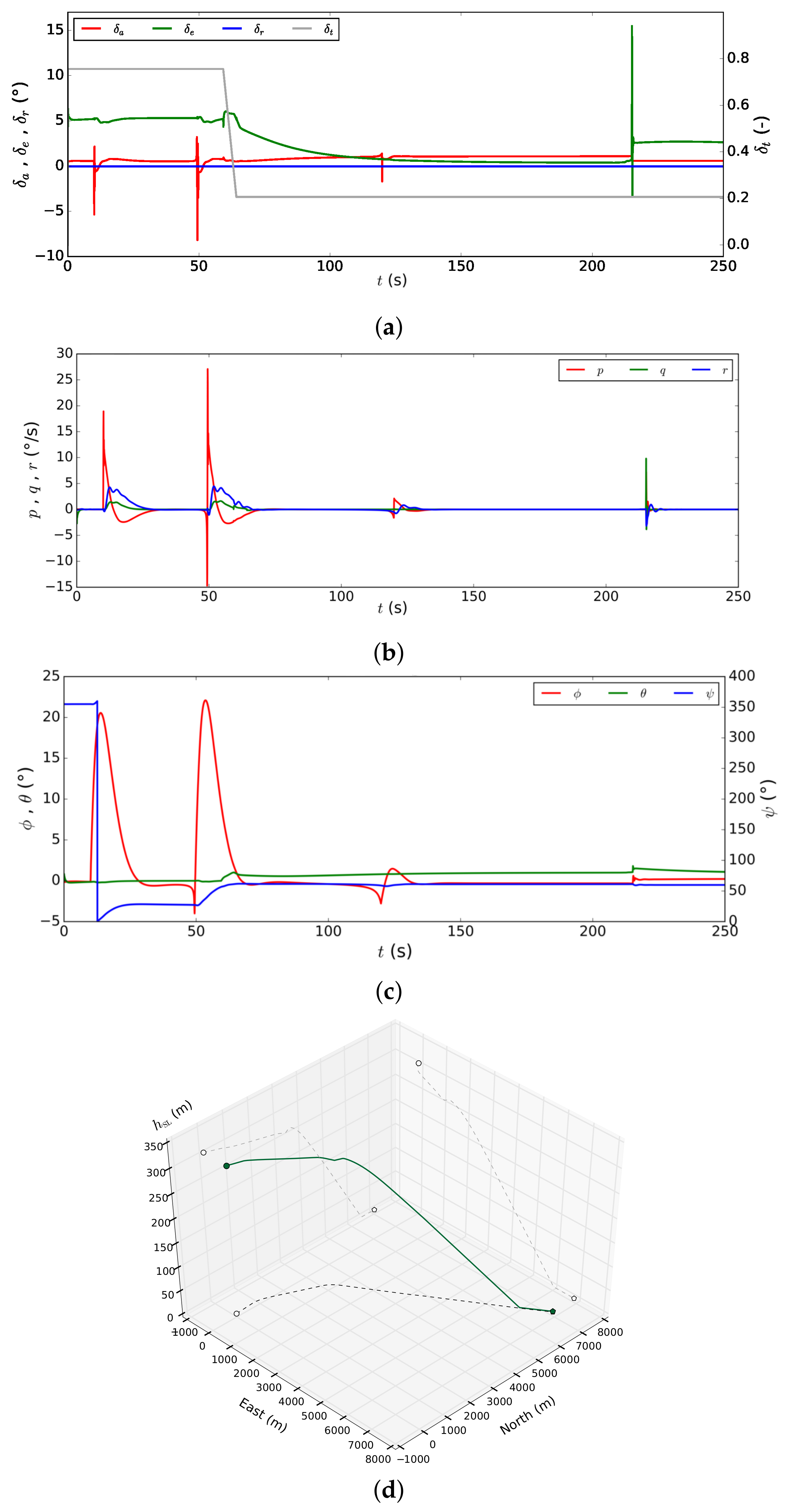
The automatic flight simulation utilities described above have been tested and validated in two phases. Initially, an alignment and landing maneuver at a specific geo-referenced runway was pursued. At this stage, focus is exclusively on 2D navigation, i.e., following a prescribed ground track, while the altitude profile was not controlled actively yet. Only one trajectory was generated from specified initial conditions, with pre-determined waypoints. The time history of control actions, together with angular rates, attitude angles and 3D trajectory, is shown in Figure 2. The three spikes along the line manifest the heading autopilot changing target. The line shows how the elevator dynamically adapts to its reference value during a turn, and then starts the descent. The final spike corresponds to touch down.
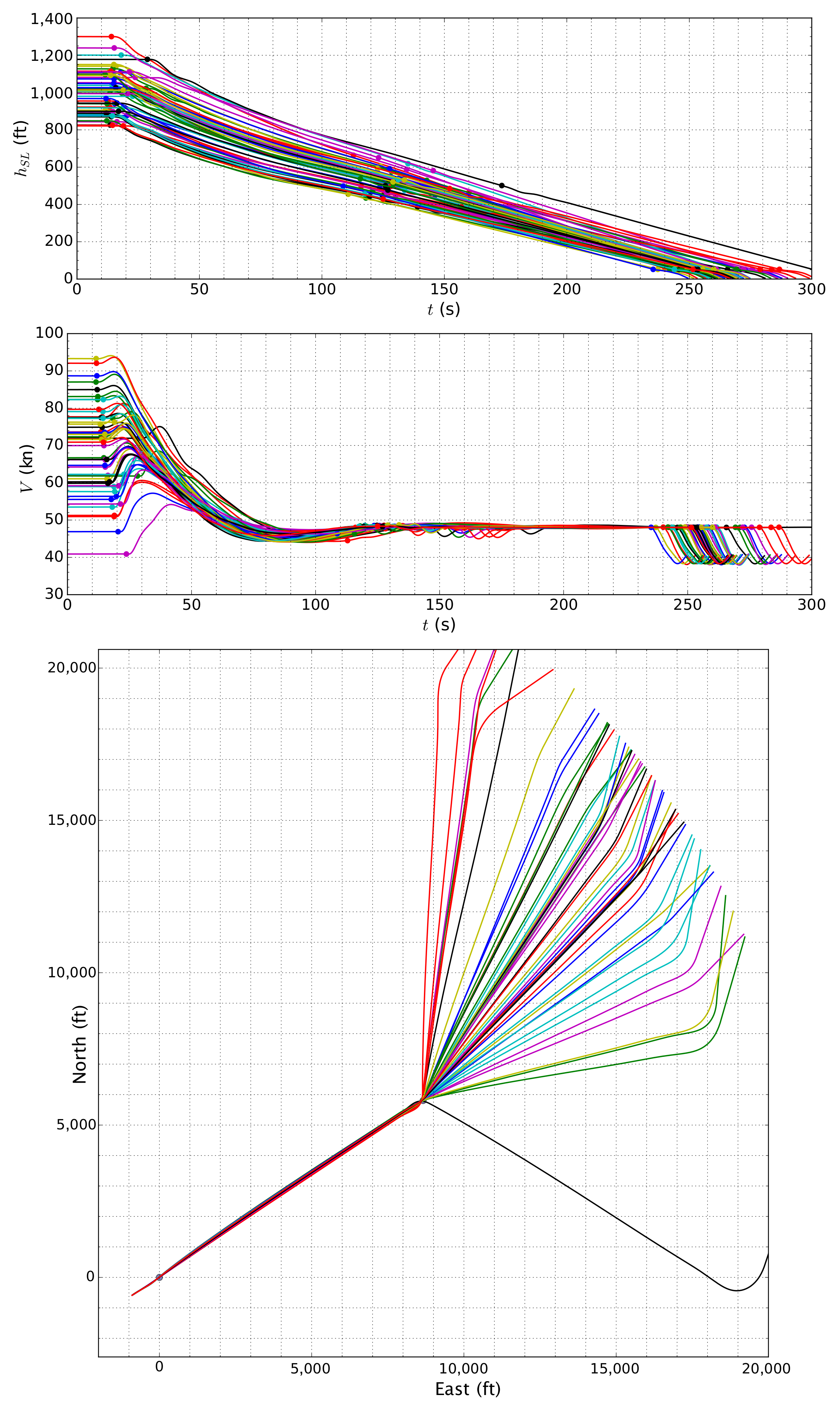
In the second phase, a very large set of simulations is generated randomly and run automatically. The way-point based navigation paradigm is again implemented, but it is now enforced with glide angle and speed control all along the trajectory. The descent and landing maneuvers are performed in a totally automatic way. The reference value for the glide angle autopilot is constantly updated since the aircraft gets below a threshold distance to the landing field; its error signal is used to control elevator deflection. In a similar fashion, speed is controlled with an auto-throttle system. Time histories for controlled altitude and speed are reported in Figure 3, together with the collection of resulting ground tracks. Markers indicate the moment the heading autopilot changes its target: first is at a distance threshold from the runway, second is for the alignment way-point, third is the field way-point. The final bump in the velocity chart manifests throttle down for counteracting ground-effect. Finally, simulation is automatically terminated at touch down. The initial position is assigned at a fixed distance to the field, with a a normally distributed azimuth angle with respect to the local North direction. For the sake of this test, the mean value was chosen to be 45, i.e., the northwest direction, and a standard deviation of 10. No matter what the random initial position is, every aircraft manages to achieve alignment with the runway and land correctly at the position . The same prescribed outcome for all simulations is achieved despite random initial conditions.
2.2. CFD Models
One of the main difficulties in direct numerical simulations with actual wind turbines geometry is represented by the different length scales of the problem. In order to resolve the full turbine geometry, ideally one would need to build a mesh with sub-millimeter resolution in the blade boundary layer inside a kilometer-scale computational box within which an entire wind-farm would fit. This issue persists also for averaging (e.g., Reynolds-Averaged Navier–Stokes, RANS) or filtered (e.g., Large Eddy Simulation, LES) techniques, where the usage of body force source terms remains the only viable simulation approach [33].
The Actuator Disk (ADM) and Actuator Line Models (ALM) [34,35] are commonly exploited to represent the wind turbine at a reduced computational cost, without resolving the full geometry of the blades. Rather, they are used to apply body forces to the flow field, in the shape of thrust and torque actions representative of the blade lift and drag forces. Both these models apply a thrust and torque on the flow, as real wind turbines actually do.
The ADM introduces a body force source in the momentum equation: this force is distributed on a permeable disk of zero thickness, and represents the rotor plane. In its simplest formulation, the actuator disc is uniformly loaded. The method has been implemented as first choice for its compatibility with a broader set of other in-house OpenFOAM libraries, expressly conceived for wind farm analysis and optimization. The most notable features include: (i) automatic meshing and mesh refining, even for complex terrain; (ii) inclusion of ground effect in the flow simulation and (iii) generation of realistic atmospheric boundary layer boundary conditions at inflow, potentially including temperature effects. The solution scheme exploits a modified version of the simpleFoam steady-state solver for incompressible and turbulent flow, i.e., for solving the RANS time-averaged equations with a modified turbulence model.
As with any axisymmetric method, the ADM is limited to averaged values of azimuthal variations on the disk surface and it is not able to simulate the wake of a single rotating blade. The number of blades and their actual rotation are, in fact, not taken into account at all. In [23,24,25], different analyses had already been carried out with this CFD approach, extracting reference data for a gust model based on current aeronautical prescriptions [14]. With this approach, the maximum angle of attack variation is related to the maximal oscillation of the velocity around its mean value at a specified distance behind the turbine. Although providing satisfying results within a model-based approach for the estimation of normal load factors due to wake encounters, this implementation of the ADM method has proven to not be sufficiently detailed to be integrated with a flight simulator for the same purpose.
For this reason, further investigations were oriented towards a more complex turbine model such as the ALM, which is able to include the transient effects present in the turbulent wake within the flight dynamics. This method exploits the same basic principle of operations of the ADM, but instead of substituting the whole rotor with a volume force distribution in the rotor disk, it represents the actual rotor blades, separately, with rotating actuator lines [36]. Volume forces are therefore distributed radially, along each one of these lines, and closely resemble the physics of a real wind turbine blade. The body forces acting on the actuator lines are computed using a blade element approach combined with tabulated two-dimensional, blade cross section, airfoil characteristics. The advantage of ALM over fully resolved geometry relies on the blades being described by span-wise distributed airfoil data, such that much fewer grid points are needed to capture the interaction of the blades with the wind field. The ALM, therefore, allows for a detailed study of the dynamics of different wake structures, such as tip and root vortices, using a reasonable number of grid nodes.
This method has been, thus, employed for the NREL 5 wind turbine model within an LES type flow simulation [37]. In the context of this research article, no detailed description of the solution techniques is reported, since these are used for the purposes of this work without any modification w.r.t. their specifications as for the highlighted literature. It features a three-bladed, upwind turbine with a rotor diameter and a nominal hub height . Its cut-in, rated and cut-out wind speeds are 3, 11.4 and 25 · respectively, and the corresponding cut-in and rated rotational speeds are 6.9 and 12.1 [38]. For each of the four experiments considered in this set of scenarios (, reported below), a 300 unsteady simulation has been run. The final time step has been then extracted and made available for the following campaign of flight simulations. For each wind speed, the appropriate rotor angular velocity has been chosen:
The cases with off-axis condition, i.e., , are considered to observe the effects of a different wake development and mixing on the flight loads of the airplane crossing behind the turbine. The computational domain extends by on the ground and 800 in altitude; it contains slightly more than 22 million cells. It features a minimum and maximum resolution of 16 and 2 , achieved with a series of three concentric cylindrical refinement regions aligned with the rotor axis and crossing the domain from side to side. Finally, the wind turbine is placed 400 inside the inflow boundary. No additional features, like complex terrain or hills and forests, were included in the domain: these would most likely increase the turbulence level downwind the turbine, but would also increase the complexity in the interpretation of the results.
Although achieving a much more detailed representation of the turbine wake in all of the above scenarios, the specific implementation of the ALM method presents some accuracy limitations, including lack of ground effect and atmospheric boundary layer, which would turn into a loss of symmetry of the wind turbine wake with respect to the its longitudinal axis, due to the vertical gradient of the wind speed. This would enhance the turbulent mixing in the near wake region, thus reducing the downwind distance where its value is maximum, see Figure 4. In this analysis, a uniform velocity profile at the inflow has been used instead. Despite the high computational cost and several approximations in the model, this method is able to capture and render the macroscopic variations of the vertical component of the flow velocity. These are interesting for they predominantly stress the most sensible aircraft flight dynamics behavior. For a verification and/or validation of the proposed simulation methodology, the reader is referred to [23,24,25,37].
2.3. Coupling, Geo-Referentiation and Wind Interpolation
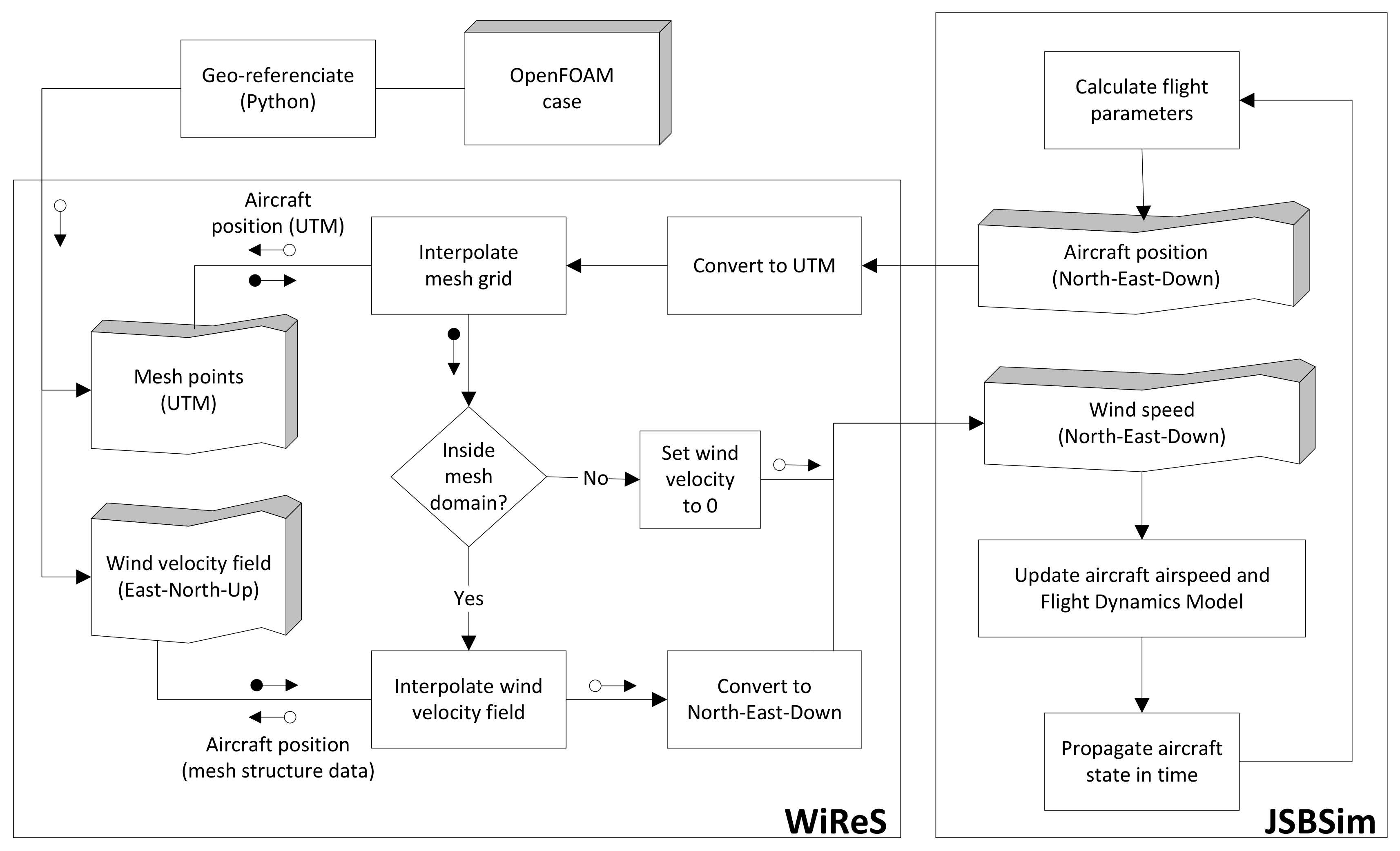
The WiReS application makes the flight and fluid dynamics sides of the simulations communicate with each other. It has been developed as an asynchronous server to work as a database and computational engine. The server is fed with the aircraft center of gravity position at every time frame of the flight dynamics simulation. It then uses this information to access the OpenFOAM mesh domain, retrieve the corresponding local wind velocity vector and send it back to the aircraft. The mesh domain and wind velocity field databases are statically loaded once and continuously accessed by the server. For this work, all of the meshes are structured and rectilinear with different local refinements regions, and it is assumed that mesh points’ coordinates are expressed in a Universal Transverse Mercator (UTM) coordinate system [39]. In order for the computational domain to represent an actual geo-referenced scenario on Earth, the mesh points must be translated according to the aircraft initial position.
The most relevant steps of the interactive process are here covered in detail. For each JSBSim instance, and for each time step in the flight dynamics simulation:
- JSBSim transmits the instantaneous aircraft position in a spherical, Earth-fixed reference frame;
- WiReS converts latitude and longitude coordinates to the UTM Cartesian coordinate system; altitude is untouched;
- WiReS uses this new form of the aircraft center of gravity position to directly access the mesh and interpolate the wind velocity vector field;
- WiReS transforms the wind velocity vector to the more common (for aeronautic applications) north-east-down reference frame and passes it back to the original instance of JSBSim;
- JSBSim acquires the wind velocity vector and uses it to update the aircraft velocity vector relative to the wind.
- Finally, all aerodynamic parameters are altered, thus taking into account the effects of the wind in that exact location on Earth, and the aircraft position is propagated to the next time frame.
The block scheme representing the whole process is represented in Figure 5. In short, along every flight trajectory, the local instantaneous wind velocity is used to alter the aircraft airspeed by interpolating the wind field at the position of the aircraft center of gravity. The wind field is considered frozen during all flight simulations and rotational effects are not included on the aircraft.
All the operations in the server scope are performed by WiReS in an asynchronous way. This turns out to be extremely useful when many JSBSim instances are launched in parallel, as the interpolation process depends on the dimension of the CFD domain and on the aircraft position relative to it.
3. Results
3.1. Scenarios Description
As explained in Section 2.2, four different CFD scenarios are well-suited to be interfaced with JSBSim. Two cases for a wind speed of 5 · and two for 12 ·, with axial and non-axial wind with respect to the turbine. The lower wind speed represents a common and realistic side wind condition in aviation; the larger serves the purpose of analyzing the effects of a completely developed wake for the turbine’s rated power condition. In all cases, wind is blowing eastwards, and its velocity distribution is considered frozen during each flight simulation. A wind axis is defined as running west to east and passing through the rotor center.
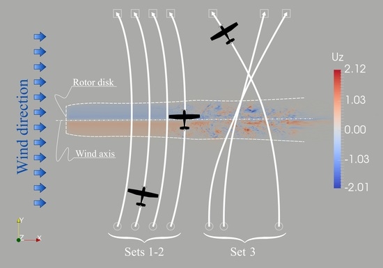
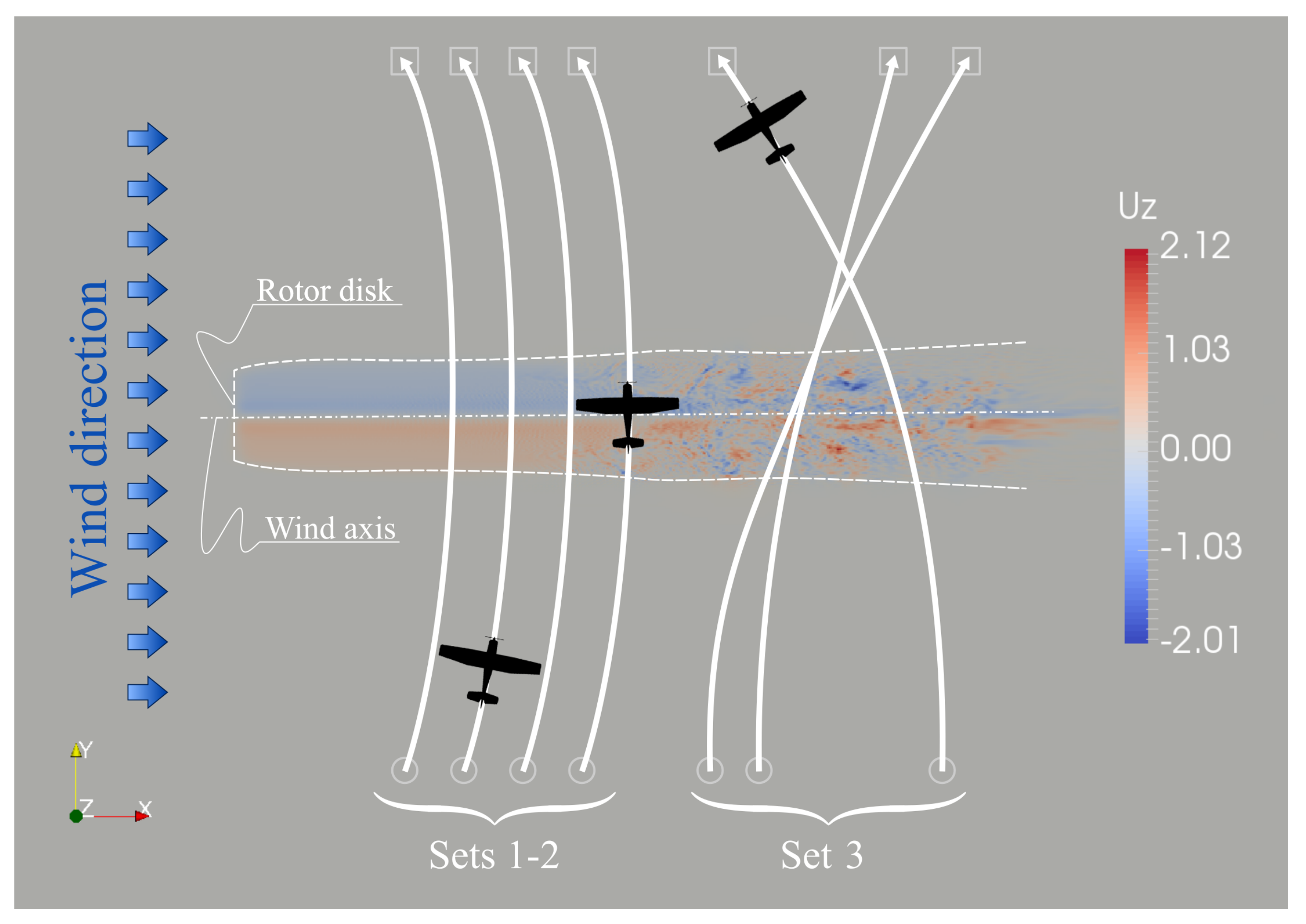
Three different templates for flight simulations were arranged for each of these CFD scenarios, for a total of twelve flight simulation families. In each template, the aircraft is positioned south of the wind axis and going north. The glide autopilot actively controls the flight path angle with elevator, while way-point navigation is implemented with ailerons. The aircraft is trimmed with flaps open in landing configuration, and in initial conditions that vary on the template case. The only part of the trajectory that is interesting for this research is the wake encounter, which typically happens midway in the flight path. JSBSim performs the trimming operation before the first time frame in the simulation, i.e., before starting the communication with WiReS, thus without any knowledge of the wind field at the initial position. As a consequence, the aircraft is exposed to an initial gust due to the wind speed at its mission starting point. In order for these undesired loads not to contaminate the effects due to gusts and turbulence of the actual wake encounter, it was necessary to set the aircraft initial position sufficiently far away from the rotor axis, thus giving the airplane the time needed to recover from the unwanted perturbed state. The key differences among the three templates are described as follows, while a representation scheme of the scenarios is reported in Figure 6.
- Set 1
- comprises 20 deterministic simulations associated with an initial aircraft speed of 50 kn (≈ 93 ·) and flight path angle equal to . Initial ground position is assigned manually with respect to the turbine disk so as to achieve crossing distances d at integer multiples of the rotor diameter, i.e., crossings at . Initial altitude is also assigned manually in order to achieve crossings exactly through the middle of the wake. Final position is symmetrical to the initial one with respect to the wind axis, and is marked by a way-point. With this set-up, the aircraft realizes an ideal wake encounter by crossing the wake at the exact wind axis and with a heading at crossing of 0 (i.e., north).
- Set 2
- resembles Set 1 in every aspect but the aircraft initial speed, which is now set to 100 kn. These first two sets are referred to as the deterministic ones, and were set-up for performing a controllable trend study on the effects of distance to the rotor and aircraft speed.
- Set 3
- is the Montecarlo set, consisting of 100 random simulations. With reference to Figure 6: (i) initial horizontal position is uniformly distributed within the region interested by the turbine wake, while vertical position is fixed at a prescribed distance from the wind axis; (ii) initial speed is also uniformly distributed between 50 and 100 kn; (iii) initial altitude is assigned as a Gaussian variable of and , where is the turbine hub height above ground; (iv) initial heading is always set to north; (v) initial flight path angle is set to ; (vi) final position way-point coordinates are assigned similarly to the initial ones; (vii) final altitude that commands the gliding autopilot at every instant is assigned to be 65 over the final way-point in all cases. In this way, the aircraft undergoes a more or less steep turn during the wake encounter, crosses the wake at different heights, incidence angle and at variable rates of descent. This attempt was meant to reproduce the natural variability lying under potential realistic wake encounter scenarios.
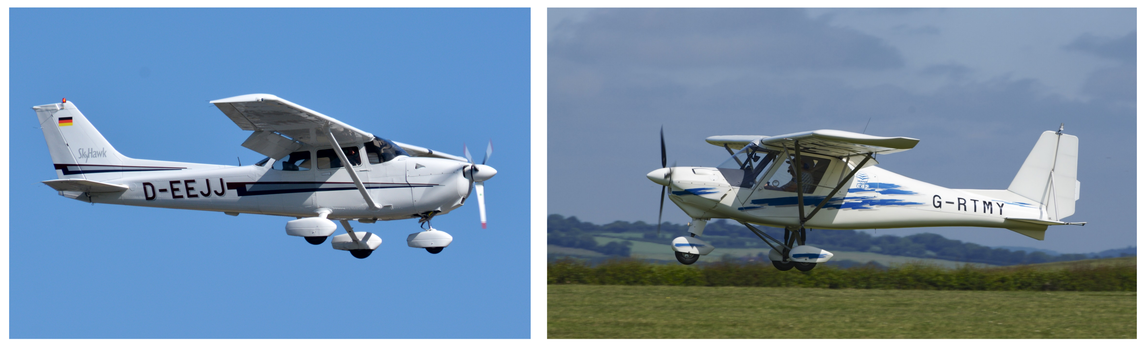
The aircraft flight dynamics model that has been implemented is a modified version of the Cessna 172 Skyhawk [40]. The original C172 implementation in JSBSim has been used since the early stages of the work, for its aerodynamic model is very consolidated, complex and reliable. The aerodynamic forces and moments acting on the aircraft are modeled by a number of build-up formulas, which are evaluated at every time-step of a flight simulation. The implementation involves the use of several look-up tables, which are entered with instantaneous values of flight parameters to evaluate all necessary quantities, such as aerodynamic, stability and control derivatives, or other effects of various types (e.g., ground effect factor). Attitude dynamics and unsteady effect on aerodynamics are not ignored: as in all the classical flight mechanics models, they are included in the form of the so called unsteady derivatives (e.g., , , etc.). For all of the coupled sets of simulation, though, the configuration model has been altered in the geometry, weight and inertia aspects, in order to better produce an acceptable representation of a lighter aircraft, namely inspired by the Ikarus C42 [41]. The previous study by the Fraunhofer IWES had already dealt with flight envelope protection of an Ikarus itself, making it reasonable to perform the simulation campaign with a vehicle from the same category of the latter [23,24,25]. Because the new aircraft is less than half as heavy as the C172, this scaling down procedure is expected to result in a worst case scenario, and is therefore supposed to provide more dramatic and interesting results. A visual comparison between the Skyhawk and Ikarus is presented in Figure 7, where it can be appreciated that they completely share the overall configuration layout and arrangement. For this reason, the JSBSim configuration file was not altered at all in the aerodynamic section, but only in the geometric and inertial ones. Two separate scaling processes have been undertaken in these two regards: they were carried out by comparing wing area and wing span for the former, and empty weight and maximum take-off weight for the latter. Two different scale factors were guessed on the basis of these comparisons and used to estimate the unknown parameters of the new aircraft. In particular, the new moments of inertia were calculated using Ikarus weight and the scaled down radius of gyration of the Cessna airplane. A recap of the main specifications of the two reference aircraft and the new modified model used within the simulations is presented in Table 1.
With being the chosen design cruise speed at sea-level altitude [14], Equation (1) prescribes that the limit positive gust load factor is for , which results in a value of for and for . In the same condition, Equation (3) is less conservative and prescribes a value of for , which means for and for . These results are summarised in Table 2. The two methods show good agreement, and in no case does the gust limit exceed the boundaries of the maneuvering limit prescribed by regulations.
3.2. Analysis of Results
Being practically homogeneous in the whole CFD domain, the macroscopic eastwards wind distribution does not strictly influence the wake encounter phase of the flight simulation. Together with the aircraft speed and flight path angle, it rather concerns some general characteristics of attitude and trajectory: ground track curvature for approaching the final way-point, pitch attitude, longer or shorter period of the initial excitation at trimming. All of these parameters are of no interest for this research, and their influence on the results of interest has been carefully neutralized by choosing the flight simulation scenarios set-up introduced in the previous section.
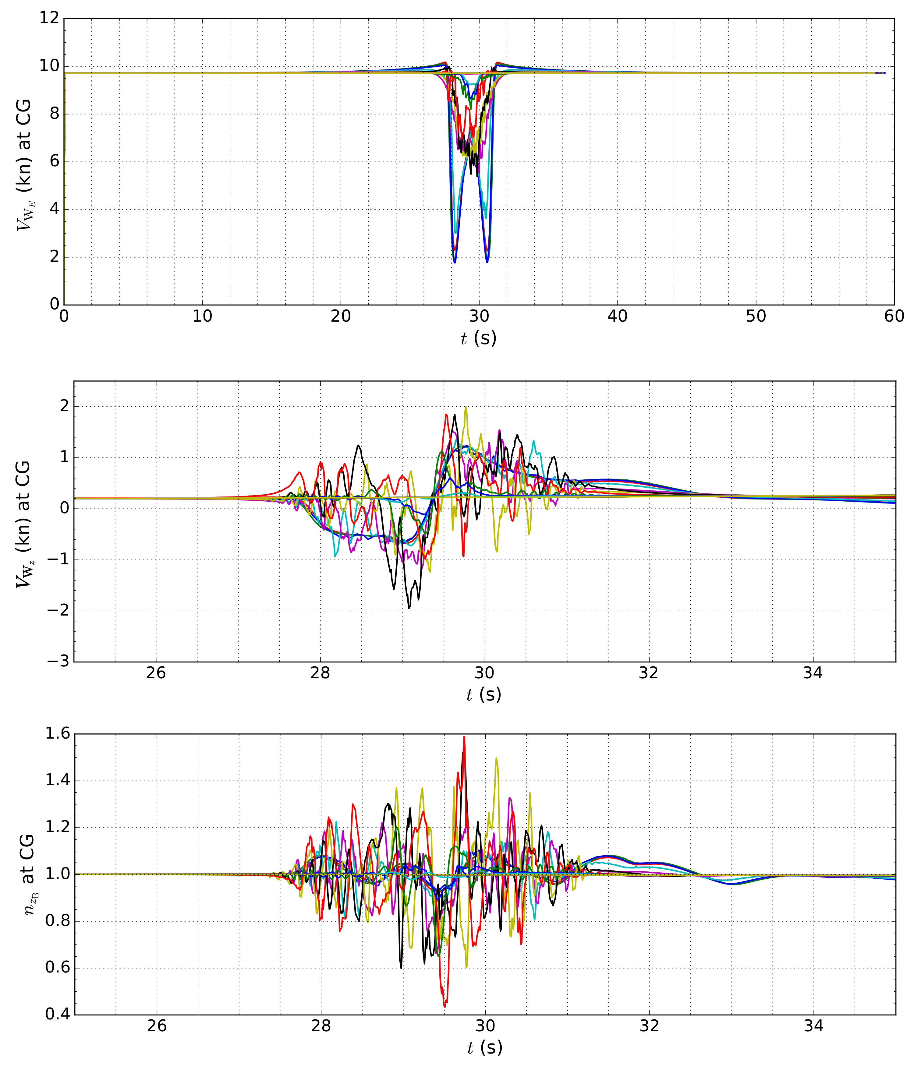
The turbine effect on the wind distribution and on the aircraft motion itself can be estimated by observing the time history of the three wind velocity field components along each one of the simulated trajectories, and in particular during the wake encounter phase. To identify the starting and ending point of the wake encounter phase for each trajectory, the axial velocity deficit downwind of the turbine rotor has been exploited. This is due to the turbine extracting kinetic energy from the wind and results in sudden decrease of axial wind speed in the area downwind the rotor (Figure 8 Top). This criterion is based on the analysis of the wind component along an Earth-fixed axis and does not depend on aircraft trajectory or attitude.
The main goal of this work is to understand in what measures rotor wake encounters affect comfort and safety of pilots of light aircraft. The focus lies on the most relevant parameters: the wind velocity component along the aircraft z-body axis , the aircraft normal load factor, along the same body axis, , and the wake encounter distance downwind the rotor. Both and are expressed in a reference frame that is fixed to the aircraft, and therefore their time history will be closely related to, and strongly dependent on, the airplane motion and attitude during the simulation.
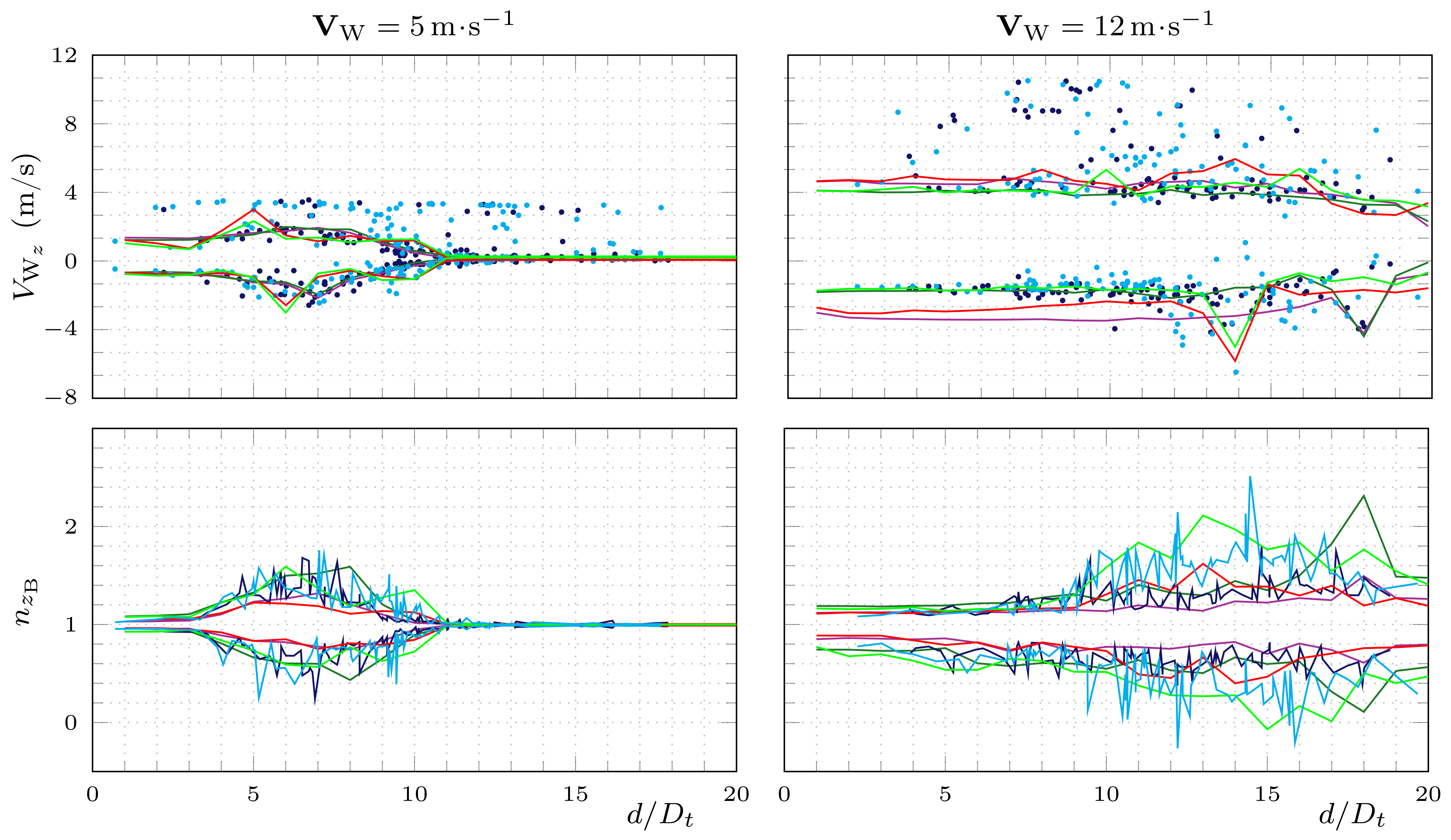
An example of the time histories of and in the wake encounter section of the trajectory is reported in Figure 8. As quantitative indicators to represent the phenomenon, the minimum and maximum of the time series have been selected. For ease of comparison among all the sets and scenarios, they are summarized in Figure 9 as a function of the normalized distance to turbine. Finally, in order to compare them with the engineering design limits imposed by regulations, and to quantitatively assess the safety level of the wake encounter, they are plotted within a realistic flight envelope diagram in Figure 10. The wind velocity vertical component is the most immediate cause that originates oscillations of the normal load factor and drives its evolution in time. In every case, there is a visible and remarkable divergence from the reference condition of . This appears both for the deterministic sets, where the aircraft is prescribed to fly exactly through the middle of the turbine wake, and for the random set, where altitude, speed and attitude at crossing are widely more fortuitous.
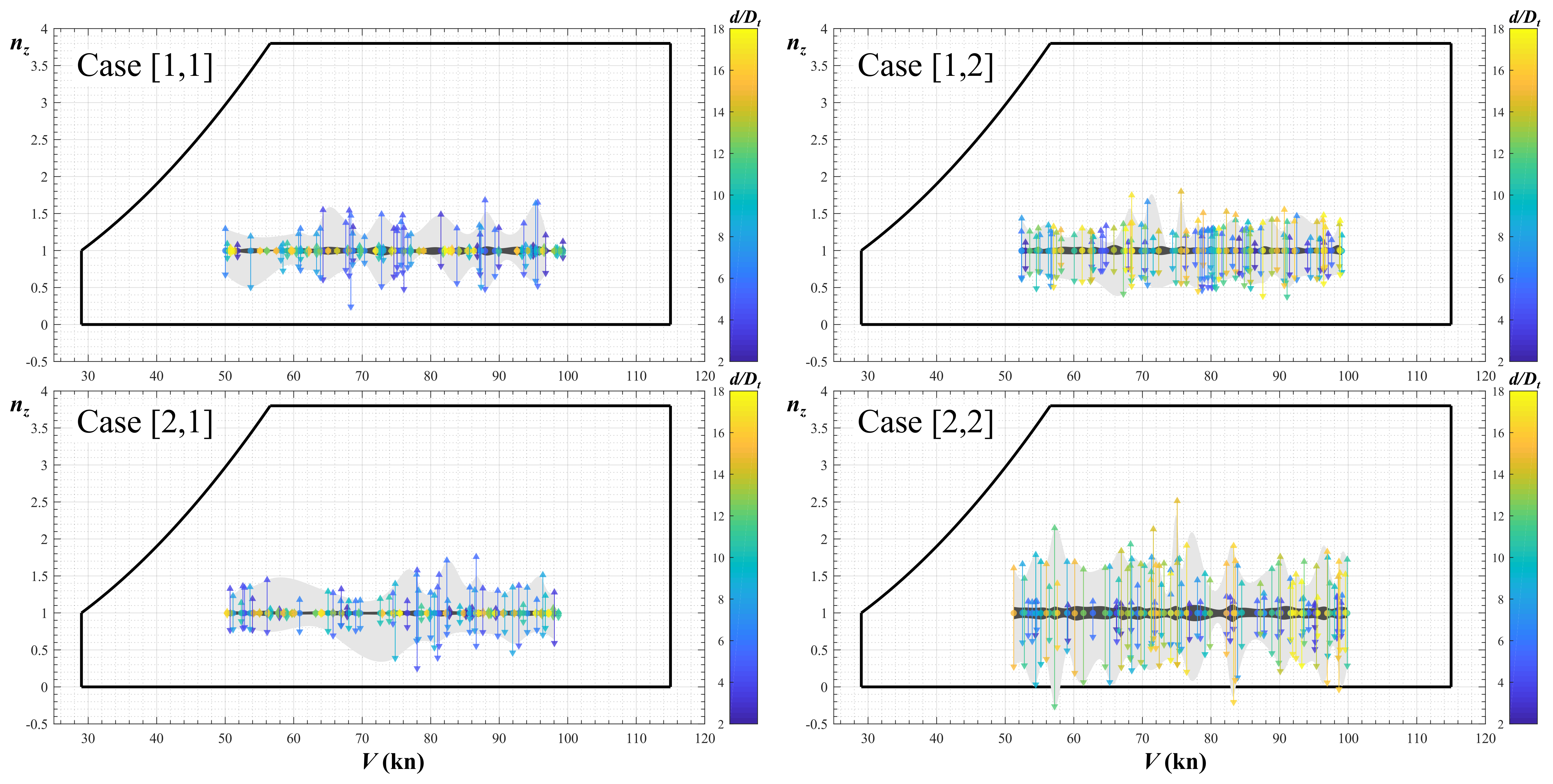
Although the extent of the normal load factor extreme values must be taken into consideration for reasons like pilot comfort and flight safety, the aircraft structural strength is not threatened at all. For the low wind speed case, the average maximum positive load factor of is equivalent to a “1-cos” natural gust of intensity encountered at aircraft speed ; for the high wind speed case, the average maximum positive load factor of corresponds to a similar encounter with ; as already reported in Section 1.2, regulations prescribe a critical value of [14].
Greater load factors almost never appear close to the turbine rotor, i.e., at a distance smaller than about depending on the wind speed. This debunks the previous conviction according to which the closer to the turbine, the more dangerous the wake encounter is for the aircraft. Instead, in all the studied cases, it appears that the region immediately downwind the rotor is characterized by only relatively small deviations of the load factor from the condition . These deviations significantly increase for crossings further away from the turbine, and seem to become maximum in amplitude in the region where the mixing between turbine wake and surrounding air is most intense and the turbulence is stronger.
The greater the aircraft speed, the more severe the wake encounter. This is manifest from the deterministic sets where, even if the wind velocity envelope is similar for the two aircraft velocity cases (or even worse for the slower one), the load factor envelope is far wider for the faster planes. This fact is easily interpreted considering that a higher speed causes a higher rate of change of the wind velocity along the trajectory, and therefore higher accelerations felt on board.
Out of axis wind conditions promote mixing and generate more turbulence, but their net effect also depends on wind speed. For the lower wind speed , the turbine wake gets easily washed out with increasing distance from the rotor, as it is not very stable even for axial wind conditions. The net effect of the misalignment is therefore less evident. For the higher wind speed of , on the other hand, it is clear how the asymmetry in the set-up of the scenario determines a very significant increase in the average spread between extreme values of the load factor, together with a notable decrease in the lowest distance at which this phenomenon happens. Out of axis conditions, therefore, make the wake encounter more concerning for a larger space interval downwind the rotor.
4. Conclusions
A neutral server platform has been developed to interface advanced open source applications for flight dynamics and CFD simulations. This software framework has been used to generate and control several populations of flight trajectories in the presence of assigned wind and turbulence fields. The purpose is a simulation-based quantification of the flight parameters involved in a wind turbine wake encounter by very-light aircraft. The flow distribution due to a modern, large horizontal axis wind turbine has been simulated in different operating conditions using the Actuator Line Model. The local instantaneous wind velocity vector and aircraft normal load factor have been monitored along every flight trajectory within several flight scenarios. The extreme values of the wind velocity and aircraft load factor components along the aircraft vertical body axis have been represented as a function of the aircraft distance downwind the rotor.
As it emerges from the results presented in the previous chapter, the instantaneous maximum and minimum values of the normal load factor increase in magnitude in the area of most intense wake mixing, at some variable distance downwind the rotor, depending on the macroscopic wind speed and direction. From 1 to 3 diameters downstream for low wind speed, and 1 to 7 diameters downstream for high wind speed, the turbine wake can still be considered stable. Although normal load factors increase with increasing aircraft speed during the wake encounter, in none of the investigated cases is the aircraft structural strength threatened at all and the flight envelope diagram is far away from the stall limits. However, the current model has a number of limitations including a very simplified model of the impact of turbulence on the aerodynamic derivatives and it does not include changes to the center of pressure during a wake encounter. Future work may want to focus on incorporating empirical flight data into the aerodynamic derivatives that can capture these dynamics since it would be very complex and prohibitive to model using CFD. The simulation platform in this paper could readily be extended to include these updates once flight data is available as well as utilizing more realistic inflow turbulent conditions.
The wake encounter dynamics are completely different whether it happens in the near or in the far wake region. This must be kept in mind as far as maneuverability and comfort on board are concerned. In the former case, the aircraft path would encounter two stable, neatly separated gusts: the first blowing upwards and the second downwards, or vice versa, depending on the turbine sense of rotation. In the latter case, the turbulent field is more chaotic, complex and distributed in space. A possible quantitative indicator to distinguish between the two phenomenons is the frequency of the wind component and normal load factors signals, as functions of time or distance traveled along the trajectory. Near-wake encounters present lower frequencies, whereas far-wake encounters present much higher ones, resulting more in continuous vibrations rather than an isolated doublet. A real world flight or a simulation test involving a pilot can provide feedback in the sense of establishing which situation is the most undesirable for human-piloted encounters. To elaborate more deeply on the effects of wake encounters on aircraft, a study of the phenomenon in the frequency domain would be an interesting challenge as well.
Acknowledgments
The simulations were performed at the HPC Cluster EDDY [44], located at the University of Oldenburg, Germany.
Author Contributions
Elia Daniele, Agostino De Marco and Bernhard Stoevesandt conceived the research. Elia Daniele, Agostino De Marco and Jonas Schmidt designed the work flow. Camine Varriale and Agostino De Marco implemented the automatic flight routines. Camine Varriale implemented the WiReS application and ran the simulations. Camine Varriale and Elia Daniele wrote the paper. Agostino De Marco, Jonas Schmidt and Bernhard Stoevesandt reviewed the paper. Bernhard Stoevesandt managed the research funding.
Conflicts of Interest
The authors declare no conflict of interest.
Nomenclature
| Angle of attack | |
| Aileron, elevator, rudder deflection | |
| Normalized throttle | |
| Mean value and standard deviation of a Gaussian distributed variable | |
| Aircraft mass factor for the computation of the limit gust load factor | |
| Air density | |
| Bank, elevation, heading angles | |
| Azimuth angle of the main wind velocity vector | |
| Azimuth angle between main wind velocity and turbine axis | |
| Shaft power | |
| a | Inertial acceleration |
| Wing span | |
| Mean aerodynamic chord length | |
| d | Downwind distance from wind turbine rotor plane |
| g | Gravitational acceleration |
| Turbine hub height | |
| Altitude above Sea Level | |
| Horizontal tail arm, | |
| Vertical tail arm, | |
| n | Normal load factor |
| Roll, pitch, yaw angular velocities | |
| t | Time |
| Position of the aerodynamic center of the horizontal tail along the x-axis in the body reference frame | |
| Position of the aerodynamic center of the vertical tail along the x-axis in the body reference frame | |
| Body reference frame | |
| Position of the center of gravity along the x-axis in the body reference frame | |
| Wind reference frame | |
| Reference gust speed | |
| Gust speed | |
| Lift coefficient | |
| Lift coefficient slope | |
| Lift coefficient derivative w.r.t. time derivative of the angle of attack | |
| Pitching moment coefficient derivative w.r.t. pitch angular velocity | |
| Turbine diameter | |
| Empirical factor for the computation of the limit gust normal load factor | |
| Central moments of inertia | |
| Turbine rotor radius | |
| S | Aircraft reference area |
| Horizontal tail area | |
| Vertical tail area | |
| Wing area | |
| V | Aircraft velocity vector |
| V | Aircraft velocity magnitude |
| Aircraft design cruise speed, design dive speed and design stall speed | |
| Aircraft vertical speed | |
| Wind velocity magnitude | |
| Wind velocity component along the axis | |
| Wind velocity component along the East direction | |
| W | Aircraft weight |
| Aircraft empty weight | |
| Aircraft maximum take-off weight | |
| B | Subscript for body reference frame |
| L | Subscript for aerodynamic lift |
| W | Subscript for wind reference frame and wind parameters |
References
- Global Wind Energy Council. Global Wind Report: Annual Market Update 2015; Global Wind Energy Council: Brussels, Belgium, 2016. [Google Scholar]
- Federal Agency for Wind Energy. Windenergieprojekte unter Berücksichtigung von Luftverkehr und Radaranlagen; Wind Energy Projects under Limitations of Aviation and Radar Facilities; Bundesverband WindEnergie e.V., Federal Agency for Wind Energy: Berlin, Germany, 2017. (In German)
- Airspace & Safety Initiative Windfarm Working Group. Managing the Impact of Wind Turbines on Aviation; Airspace & Safety Initiative Windfarm Working Group: Hampshire, UK, 2013. [Google Scholar]
- U.S. Department of Transportation—Federal Aviation Administration. Recommended Standard Traffic Patterns and Practices for Aeronautical Operations at Airports without Operating Control Towers; U.S. Department of Transportation: Washington, DC, USA, 1993.
- Keränen, R.; Pettazzi, A.; Alku Catalina, L.; Salsón, S. Weather Radar and Abundant Wind Farmin—Impacts on Data Quality and Mitigation by Doppler Dual-Polarization. In Proceedings of the ERAD2014 8th European Conference on Radar in Meteorology and Hydrology, Garmisch-Partenkirchen, Germany, 1–5 September 2014. [Google Scholar]
- Gilman, P.; Husser, L.; Miller, B.; Peterson, L. Federal Interagency Wind Turbine Radar Interference Mitigation Strategy; Report for U.S. Department of Energy; U.S. Department of Energy: Washington, DC, USA, 2016.
- Hall, W.; Rico-Ramirez, M.A.; Krämer, S. Offshore wind turbine clutter characteristics and identification in operational C–band weather radar measurements. Q. J. R. Metereol. Soc. 2017, 143, 720–730. [Google Scholar] [CrossRef]
- European Aviation Safety Agency (EASA). Annual Aviation Safety Review; EASA: Cologne, Germany, 2017. [Google Scholar]
- Bureau of Aircraft Accidents Archives (B3A). Available online: http://www.baaa-acro.com (accessed on 5 April 2018).
- Glabeke, G. The Influence of Wind Turbine Induced Turbulence on Ultralight Aircraft, a CFD Analysis. Ph.D. Thesis, VIVES University of Applied Sciences, Oostende, Belgium, 2011. [Google Scholar]
- Van der Wall, B.; Fischenberg, D.; Lehmann, P.; van der Wall, L. Impact of Wind Energy Rotor Wakes on Fixed-Wing Aircraft and Helicopters. In Proceedings of the 42nd European Rotorcraft Forum, Lille, France, 5–8 September 2016. [Google Scholar]
- Mulinazzi, T.E.; Zheng, Z. Wind Farm Turbulence Impacts on General Aviation Airports in Kansas; Kansas Department of Transportation: Topeka, KS, USA, 2014.
- Wang, Y.; White, M.; Barakos, G. Wind Turbine Wake Encounter Study; Civil Aviation Authority: London, UK, 2015.
- European Aviation Safety Agency. EASA Certification Specifications for Very Light Aeroplanes; EASA: Cologne, Germany, 2003. [Google Scholar]
- Sanderse, B.; van der Pijl, S.; Koren, B. Review of computational fluid dynamics for wind turbine wake aerodynamics. Wind Energy 2011, 14, 799–819. [Google Scholar] [CrossRef]
- Carrión, M.; Woodgate, M.; Steijl, R.; Barakos, G.N.; Gomez-Iradi, S.; Munduate, X. Understanding wind-turbine wake breakdown using computational fluid dynamics. AIAA J. 2015, 53, 588–602. [Google Scholar] [CrossRef]
- Troldborg, N.; Zahle, F.; Sørensen, N.; Réthoré, P. Comparison of wind turbine wake properties in non-uniform inflow predicted by different rotor models. J. Phys. Conf. Ser. 2014, 555, 012100. [Google Scholar] [CrossRef]
- Kalvig, S.; Manger, E.; Hjertager, B. Comparing different CFD wind turbine modelling approaches with wind tunnel measurements. J. Phys. Conf. Ser. 2014, 555. [Google Scholar] [CrossRef]
- Martínez-Tossas, L.A.; Churchfield, M.J.; Leonardi, S. Large Eddy Simulations of the flow past wind turbines: Actuator line and disk modeling. Wind Energy Wiley Online Libr. 2015, 8, 1047–1060. [Google Scholar] [CrossRef]
- Martinez, L.; Leonardi, S.; Churchfield, M.; Moriarty, P. A Comparison of Actuator Disk and Actuator Line wind turbine models and best practices for their use. In Proceedings of the 50th AIAA Aerospace Sciences Meeting including the New Horizons Forum and Aerospace Exposition, Nashville, TN, USA, 9–12 January 2012. [Google Scholar]
- Hardin, J. The velocity field induced by a helical vortex filament. Phys. Fluids 1982, 25. [Google Scholar] [CrossRef]
- Kocurek, D. Lifting Surface Performance Analysis for Horizontal Axis Wind Turbines; Solar Energy Research Institute: Golden, CO, USA, 1987. [Google Scholar]
- Schmidt, J.; Daniele, E.; Stoevesandt, B. Böenbelastung von UL-Flugzeugen durch den Turbulenten Nachlauf von Windenergieanlagen; Internal Report; Fraunhofer-Institute for Wind Energy Systems (IWES): Oldenburg, Germany, 2015. (In German) [Google Scholar]
- Schmidt, J.; Daniele, E.; Stoevesandt, B. Ergänzende Ergebnisauswertung zur Gefährdung von ULF durch WEA für den Standort Linnich-Boslar; Internal Report; Fraunhofer-Institute for Wind Energy Systems (IWES): Oldenburg, Germany, 2015. (In German) [Google Scholar]
- Schmidt, J.; Daniele, E.; Stoevesandt, B. Preliminary Assessment of the Impact of the Fairview Wind Project on Small Aircrafts at the Stayner Aerodrome; Internal Report; Fraunhofer-Institute for Wind Energy Systems (IWES): Oldenburg, Germany, 2016. [Google Scholar]
- Padfield, G.; Manimala, B.; Turner, G. A Severity Analysis for Rotorcraft Encounters with Vortex Wakes. J. Am. Helicopter Soc. 2004, 49, 445–456. [Google Scholar] [CrossRef]
- De Marco, A.; D’Auria, J. Collision Risk Studies with 6DOF Flight Simulations when Aerodrome Obstacle Standards Cannot Be Met. In Proceedings of the 29th Congress of the International Council of the Aeronautical Sciences (ICAS 2014), St. Petersburg, Russia, 7–12 September 2014. [Google Scholar]
- JSBSim: An Open Source, Platform-Independent, Flight Dynamics & Control Software Library in C++. Available online: http://jsbsim.sourceforge.net/ (accessed on 10 April 2018).
- OpenFOAM, Free CFD Software, The OpenFOAM Foundation. Available online: https://openfoam.org/ (accessed on 10 April 2018).
- Project Jupyter. Available online: http://jupyter.org/ (accessed on 10 April 2018).
- GitHub of the Aircraft Design Group of the University of Naples Federico II. Available online: https://github.com/Aircraft-Design-UniNa/WiReS (accessed on 10 April 2018).
- Ziegler, J.G.; Nichols, N.B.; Rochester, N.Y. Optimum Settings for Automatic Controllers. Trans. ASME 1942, 64, 759–765. [Google Scholar] [CrossRef]
- Vollmer, L.; van Dooren, M.; Trabucchi, D.; Schneemann, J.; Steinfeld, G.; Witha, B.; Trujillo, J.; Kühn, M. First comparison of LES of an offshore wind turbine wake with dual-Doppler lidar measurements in a German offshore wind farm. J. Phys. Conf. Ser. 2015, 625. [Google Scholar] [CrossRef]
- Mikkelsen, R. Actuator Disc Methods Applied to Wind Turbines. Ph.D. Thesis, Technical University of Denmark, Kongens Lyngby, Denmark, 2004. [Google Scholar]
- Jha, P.K.; Churchfield, M.J.; Moriarty, P.J.; Schmitz, S. Guidelines for Volume Force Distributions within Actuator Line Modeling of Wind Turbines on Large-Eddy Simulation-Type Grids. J. Sol. Energy Eng. 2014, 136, 031003. [Google Scholar] [CrossRef]
- Troldborg, N.; Sørensen, J.; Mikkelsen, R. Actuator Line Modeling of Wind Turbine Wakes. Ph.D. Thesis, Technical University of Denmark, Kongens Lyngby, Denmark, 2009. [Google Scholar]
- Rahimi, H.; Garcia, A.M.; Stoevesandt, B.; Peinke, J.; Schepers, G. An engineering model for wind turbines under yawed conditions derived from high fidelity models. Wind Energy 2018. [Google Scholar] [CrossRef]
- Jonkman, J.; Butterfield, S.; Musial, W.; Scott, G. Definition of a 5-MW Reference Wind Turbine for Offshore System Development; NREL/TP-500-38060; National Renewable Energy Laboratory: Golden, CO, USA, 2009.
- Snyder, J. Map Projections—A Working Manual; United States Governmental Printing Office: Washington, DC, USA, 1983.
- Cessna C172 Skyhawk Specifications. Available online: http://cessna.txtav.com/en/piston/cessna-skyhawk (accessed on 10 April 2018).
- Comco Ikarus C42 Specifications. Available online: http://www.comco-ikarus.de/Pages/produkte-comco/c42a.php (accessed on 10 April 2018).
- Foto by Frank Schwichtenberg (CC BY-SA 3.0). Available online: https://commons.wikimedia.org/wiki/File%3ACessna_172R_Skyhawk_(D-EEJJ)_04.jpg (accessed on 10 April 2018).
- Foto by Ian Kirk from Broadstone, Dorset, UK (CC BY 2.0). Available online: https://commons.wikimedia.org/wiki/File%3AIkarus_C42_Compton_Abbas_30th_June_2013_(9218593234).jpg (accessed on 10 April 2018).
- HPC Cluster EDDY. Available online: www.uni-oldenburg.de/fk5/wr/hochleistungsrechnen/hpc-facilities/eddy/ (accessed on 10 April 2018).
Figure 1.
Qualitative V-n diagram for light and very light aircraft. Only positive load factors are represented. If the maximum load factor arising during a turbine wake encounter falls in the area within the red hatching, the encounter can be considered safe.
Figure 1.
Qualitative V-n diagram for light and very light aircraft. Only positive load factors are represented. If the maximum load factor arising during a turbine wake encounter falls in the area within the red hatching, the encounter can be considered safe.

Figure 2.
(a) time histories of the total actions on the aircraft four main control devices: ![Aerospace 05 00042 i001]() aileron ,
aileron , ![Aerospace 05 00042 i002]() elevator ,
elevator , ![Aerospace 05 00042 i003]() rudder and
rudder and ![Aerospace 05 00042 i004]() throttle , on the right vertical axis. These are the superposition of the initial trim command and autopilots actions; (b) time histories of the angular speed components in body axes:
throttle , on the right vertical axis. These are the superposition of the initial trim command and autopilots actions; (b) time histories of the angular speed components in body axes: ![Aerospace 05 00042 i001]() roll rate p,
roll rate p, ![Aerospace 05 00042 i002]() pitch rate q and
pitch rate q and ![Aerospace 05 00042 i003]() yaw rate r; (c) time histories of the Euler angles:
yaw rate r; (c) time histories of the Euler angles: ![Aerospace 05 00042 i001]() bank angle ,
bank angle , ![Aerospace 05 00042 i002]() elevation-angle and
elevation-angle and ![Aerospace 05 00042 i003]() heading angle on the right vertical axis; and (d) 3D representation of the trajectory, with ground track and side-view projections. Altitude is not to scale.
heading angle on the right vertical axis; and (d) 3D representation of the trajectory, with ground track and side-view projections. Altitude is not to scale.
 aileron ,
  elevator ,
  rudder and
  throttle , on the right vertical axis. These are the superposition of the initial trim command and autopilots actions; (b) time histories of the angular speed components in body axes: roll rate p, pitch rate q and yaw rate r; (c) time histories of the Euler angles: bank angle , elevation-angle and heading angle on the right vertical axis; and (d) 3D representation of the trajectory, with ground track and side-view projections. Altitude is not to scale.
Figure 2.
(a) time histories of the total actions on the aircraft four main control devices: ![Aerospace 05 00042 i001]() aileron ,
aileron , ![Aerospace 05 00042 i002]() elevator ,
elevator , ![Aerospace 05 00042 i003]() rudder and
rudder and ![Aerospace 05 00042 i004]() throttle , on the right vertical axis. These are the superposition of the initial trim command and autopilots actions; (b) time histories of the angular speed components in body axes:
throttle , on the right vertical axis. These are the superposition of the initial trim command and autopilots actions; (b) time histories of the angular speed components in body axes: ![Aerospace 05 00042 i001]() roll rate p,
roll rate p, ![Aerospace 05 00042 i002]() pitch rate q and
pitch rate q and ![Aerospace 05 00042 i003]() yaw rate r; (c) time histories of the Euler angles:
yaw rate r; (c) time histories of the Euler angles: ![Aerospace 05 00042 i001]() bank angle ,
bank angle , ![Aerospace 05 00042 i002]() elevation-angle and
elevation-angle and ![Aerospace 05 00042 i003]() heading angle on the right vertical axis; and (d) 3D representation of the trajectory, with ground track and side-view projections. Altitude is not to scale.
heading angle on the right vertical axis; and (d) 3D representation of the trajectory, with ground track and side-view projections. Altitude is not to scale.
aileron , elevator , rudder and throttle , on the right vertical axis. These are the superposition of the initial trim command and autopilots actions; (b) time histories of the angular speed components in body axes: roll rate p, pitch rate q and yaw rate r; (c) time histories of the Euler angles: bank angle , elevation-angle and heading angle on the right vertical axis; and (d) 3D representation of the trajectory, with ground track and side-view projections. Altitude is not to scale.
Figure 3.
Time histories of altitude above Mean Sea Level (Top) and of velocity magnitude (Middle) for a set of 50 flight simulations. Although starting with random initial conditions, all aircraft arrive at the landing field with a final altitude of exactly 50 (i.e., the prescribed obstacle height) and the same prescribed speed; (Bottom) ground tracks for the same set of 50 flight simulations. Despite the random intial position, all aircraft correctly pass through the alignment checkpoint and land at (0,0) position.

Figure 4.
Velocity color plots for the Actuator Line Model (ALM), top views. Wind blows eastwards, while rotor axis is rotated 15 north with respect to West direction (left-hand side of the pictures). (Top) Magnitude of flow velocity for the case ; (Bottom) Vertical component of flow velocity for the case : the two opposite contributions of the ascending and descending blade are relevant and evident. The downstream distance normalized with the rotor diameter is reported on the x-axes.

Figure 5.
Block scheme representing the interaction among JSBSim, WiReS and OpenFOAM.

Figure 6.
Scenarios scheme for a comparison of the three simulation families. The background image shows the wind velocity’s vertical component field for the OpenFOAM case . Aircraft silhouette is not to scale and all of the three sets investigate the aircraft behaviour on the whole extension of the wake downwind of the turbine.


Figure 8.
Time histories for case and Set 2. (Top) wind velocity component along the east direction, which is not dependent on the aircraft attitude. The whole trajectory, from start to end, is covered in the plots. The wake encounter phase is clearly rendered by the pronounced decrease in magnitude, about midway through the trajectory. For a few trajectories closer to the rotor disk, it is possible to distinguish the two separate wakes due to the actual blades; (Middle and Bottom) wind velocity component and aircraft normal load factor along the body-fixed axis. These quantities depend on the actual attitude of the aircraft and only the wake encounter section of the trajectory is reported. The trajectories that are closer to the wind turbine are characterized by a lower frequency in the oscillations of both and , due to the stability of the near wake.

Figure 9.
Maximum and minimum values of the wind velocity components along the aircraft axis and the consequently arisen normal load factor , presented as a function of the normalized distance from the turbine rotor along the wind axis. Wrap of the deterministic Sets 1, 2 and the random Set 3 for all cases. Legend for all diagrams: ![Aerospace 05 00042 i005]() 50 kn in-axis;
50 kn in-axis; ![Aerospace 05 00042 i002]() 100 kn in-axis;
100 kn in-axis; ![Aerospace 05 00042 i001]() 50 kn off-axis;
50 kn off-axis; ![Aerospace 05 00042 i006]() 100 kn off-axis;
100 kn off-axis; ![Aerospace 05 00042 i007]() Sets 3 in-axis;
Sets 3 in-axis; ![Aerospace 05 00042 i008]() Sets 3 off-axis.
Sets 3 off-axis.
 50 kn in-axis; 100 kn in-axis; 50 kn off-axis;
  100 kn off-axis;
  Sets 3 in-axis;
  Sets 3 off-axis.
Figure 9.
Maximum and minimum values of the wind velocity components along the aircraft axis and the consequently arisen normal load factor , presented as a function of the normalized distance from the turbine rotor along the wind axis. Wrap of the deterministic Sets 1, 2 and the random Set 3 for all cases. Legend for all diagrams: ![Aerospace 05 00042 i005]() 50 kn in-axis;
50 kn in-axis; ![Aerospace 05 00042 i002]() 100 kn in-axis;
100 kn in-axis; ![Aerospace 05 00042 i001]() 50 kn off-axis;
50 kn off-axis; ![Aerospace 05 00042 i006]() 100 kn off-axis;
100 kn off-axis; ![Aerospace 05 00042 i007]() Sets 3 in-axis;
Sets 3 in-axis; ![Aerospace 05 00042 i008]() Sets 3 off-axis.
Sets 3 off-axis.
50 kn in-axis; 100 kn in-axis; 50 kn off-axis; 100 kn off-axis; Sets 3 in-axis; Sets 3 off-axis.
Figure 10.
V-n diagram in the positive load factor semi-plane for the custom modelled aircraft. Design stall speed in clean configuration is kn, design cruise speed is kn and dive speed is kn. The positive limit maneuvering load factor is . The maximum (), minimum () and average () values of the aircraft normal load factor are plotted at the corresponding wake encounter speed for the random Set 3 of each of the four cases. The color grading indicates the normalized distance downwind the turbine at which the crossing has taken place. The light grey background highlights the clusters of data that presents positive or negative peak values. The dark grey area along the line envelopes the load factor values contained within the interval . From this visualization, it is more clear that the wake encounter as simulated in this work poses no threat for the control and structural safety of the aircraft.


Table 1.
Main specifications of the reference aircraft and the custom version used for the simulation campaign. Geometric data is estimated via a scale factor based on and ; weights and inertia are estimated via a different scale factor based on and .
Table 1.
Main specifications of the reference aircraft and the custom version used for the simulation campaign. Geometric data is estimated via a scale factor based on and ; weights and inertia are estimated via a different scale factor based on and .
| Cessna 172 | Ikarus C42 | Custom | Units | |||||
|---|---|---|---|---|---|---|---|---|
| Seats | 4 | 2 | 2 | – | ||||
| 174 | (16.2) | 135 | (12.5) | 142 | (13.2) | () | ||
| 36.1 | (11) | 31.0 | (9.45) | 29.5 | (9.00) | () | ||
| 4.9 | (1.5) | – | 4.0 | (1.2) | () | |||
| 21.9 | (2.03) | – | 17.9 | (1.66) | () | |||
| 15.7 | (4.78) | – | 12.9 | (3.93) | () | |||
| 16.5 | (1.53) | – | 13.5 | (1.25) | () | |||
| 15.7 | (4.78) | – | 12.9 | (3.93) | () | |||
| 1640 | (744) | 583 | (264) | 596 | (270) | () | ||
| 2550 | (1157) | 1041 | (472) | – | () | |||
| 948 | (1285) | – | 261 | (353) | () | |||
| 1346 | (1825) | – | 371 | (503) | () | |||
| 1967 | (2667) | – | 542 | (735) | () | |||
| 180 | (134) | 100 | (75) | 100 | (75) | () | ||
© 2018 by the authors. Licensee MDPI, Basel, Switzerland. This article is an open access article distributed under the terms and conditions of the Creative Commons Attribution (CC BY) license (http://creativecommons.org/licenses/by/4.0/).
Share and Cite
MDPI and ACS Style
Varriale, C.; De Marco, A.; Daniele, E.; Schmidt, J.; Stoevesandt, B. Flight Load Assessment for Light Aircraft Landing Trajectories in Windy Atmosphere and Near Wind Farms. Aerospace 2018, 5, 42. https://doi.org/10.3390/aerospace5020042
AMA Style
Varriale C, De Marco A, Daniele E, Schmidt J, Stoevesandt B. Flight Load Assessment for Light Aircraft Landing Trajectories in Windy Atmosphere and Near Wind Farms. Aerospace. 2018; 5(2):42. https://doi.org/10.3390/aerospace5020042
Chicago/Turabian StyleVarriale, Carmine, Agostino De Marco, Elia Daniele, Jonas Schmidt, and Bernhard Stoevesandt. 2018. "Flight Load Assessment for Light Aircraft Landing Trajectories in Windy Atmosphere and Near Wind Farms" Aerospace 5, no. 2: 42. https://doi.org/10.3390/aerospace5020042
Note that from the first issue of 2016, this journal uses article numbers instead of page numbers. See further details here.