Simulation and Modeling of Rigid Aircraft Aerodynamic Responses to Arbitrary Gust Distributions


1
High Performance Computing Research Center, U.S. Air Force Academy, Air Force Academy, CO 80840, USA
2
Department of Mechanical and Aerospace Engineering, University of Colorado at Colorado Springs, Colorado Springs, CO 80918, USA
*
Author to whom correspondence should be addressed.
Aerospace 2018, 5(2), 43; https://doi.org/10.3390/aerospace5020043
Submission received: 19 March 2018
/
Revised: 9 April 2018
/
Accepted: 14 April 2018
/
Published: 18 April 2018
(This article belongs to the Special Issue Computational Aerodynamic Modeling of Aerospace Vehicles)
Abstract
:The stresses resulting from wind gusts can exceed the limit value and may cause large-scale structural deformation or even failure. All certified airplanes should therefore withstand the increased loads from gusts of considerable intensity. A large factor of safety will make the structure heavy and less economical. Thus, the need for accurate prediction of aerodynamic gust responses is motivated by both safety and economic concerns. This article presents the efforts to simulate and model air vehicle aerodynamic responses to various gust profiles. The computational methods developed and the research outcome will play an important role in the airplane’s structural design and certification. Cobalt is used as the flow solver to simulate aerodynamic responses to wind gusts. The code has a user-defined boundary condition capability that was tested for the first time in the present study to model any gust profile (intensity, direction, and duration) on any arbitrary configuration. Gust profiles considered include sharp edge, one minus cosine, a ramp, and a 1-cosine using tabulated data consisting of gust intensity values at discrete time instants. Test cases considered are a flat plate, a two-dimensional NACA0012 airfoil, and the high Reynolds number aero-structural dynamics (HIRENASD) configuration, which resembles a typical large passenger transport aircraft. Test cases are assumed to be rigid, and only longitudinal gust profiles are considered, though the developed codes can model any gust angle. Time-accurate simulation results show the aerodynamic responses to different gust profiles including transient solutions. Simulation results show that sharp edge responses of the flat plate agree well with the Küssner approximate function, but trends of other test cases do not match because of the thin airfoil assumptions made to derive the analytical function. Reduced order aerodynamic models are then created from the convolution integral of gust amplitude and the time-accurate responses to sharp-edge gusts. Convolution models are next used to predict aerodynamic responses to arbitrary gust profiles without the need of running time-accurate simulations for every gust shape. The results show very good agreement between developed models and simulation data.
1. Introduction
Currently, the use of computational fluid dynamic (CFD) solutions is considered the state of the art in modeling unsteady nonlinear flow physics and offers an early and improved understanding of vehicle aerodynamics. In addition, these predictions can improve the accuracy of the structural analysis, performance predictions, and flight control design. This translates into reduced project risk and enhanced analysis of system performance prior to prototyping and first flight. The use of high fidelity aerodynamic simulations reduces the number of physical models and wind tunnel tests required until the design process converges to a design that optimizes an objective function, satisfies all mission requirements, and meets airworthiness standards. Specifically, the aircraft design should ensure the structural integrity in the presence of wind gusts of considerable intensity.
Calm atmospheric conditions rarely exist because of the continuous presence of random fluctuations in wind speed and direction. Wind gusts, in general, have continuous and random distributions and can occur in different directions. These gust profiles are described with the power spectral density technique. Sometimes, gust distributions can be represented as a discrete single function such as “one minus cosine”. The impacts of these gusts (continuous and discrete) on the aerodynamics and structure of airplanes should be understood in order to improve the safety and functionality of designs economically. In particular, the aerodynamic responses to wind gusts are important for low-altitude and high-speed flight conditions or for large-size flexible aircraft with small natural frequencies [1]. FAR 25 (Federal Aviation Regulations, Part 25) requires that transport airplane structures should withstand the presence of static loads due to discrete gusts of 1-cosine with a length of 12.5 wing chord and a prescribed velocity at different flight envelope conditions [2]. In addition, the airplane should be certified when dynamic gust loads described by the power spectral density technique are encountered. A large factor of safety will make the structure heavy and less economical. Thus, the need for accurate prediction of aerodynamic gust responses is motivated by both safety and economic concerns.
Limited analytical solutions are available for gust predictions of two-dimensional test cases. Küssner [3] was the first to calculate the indicial lift response of a flat plate to a vertical sharp-edge gust in incompressible flow; his solution is known as the Küssner function. The Küssner function can be approximated by an exponential series as reported by Jones [4] for incompressible flow or by Mazelsky and Drischle [5] for compressible flow. As another example, Von Karman & Sears [6] derived the frequency response to a sinusoidal gust. Note that these theories are limited only to potential flow and a thin airfoil traversing gusts of low intensity. Techniques for gust generation in wind tunnels are complicated; initial efforts were made to generate an oscillating gust in the wind tunnel using a two-dimensional plunging airfoil mounted upstream of the test section [7]. Bennett and Gilman [1] described a gust generation method tested in the NASA Langley Transonic Dynamics Tunnel that used deflecting vanes. Compte-Bellot and Corrsin [8] used a hot wire technique to generate isotropic homogeneous turbulence in a wind tunnel. All these techniques are limited on the length scale of generated turbulence [9]. In addition, wind tunnel and flight testing are quite expensive and typically available late in the aircraft design stage. An alternative is the simulation of wind gust using computational methods with even further cost savings noticed by using a reduced order model.
The common industrial practice in computing the impacts of wind gusts on the aircraft structure is to use the double lattice method or strip theory [10]. However, these methods are not accurate in modeling nonlinear aerodynamics, e.g., the transonic regime, or when the viscosity effects are important. There are limited studies of wind gusts using solutions of the unsteady Reynolds-averaged Navier–Stokes (URANS) equations. This is because wind gust modeling is not typically available in most commercial CFD codes. A few methods of time-accurate simulations of wind gust are described in [11,12,13,14,15,16,17,18]. One approach is to add an artificial local gust velocity to each cell flow velocity [18,19]. The method can model any gust shape and the gust simulations can begin from the time that gust hits the most forward point of the vehicle. However, the technique is not available in commercial codes. Similar to analytical solutions, the method does not consider any effect of the vehicle on the gust profile. Another common approach to model gust in CFD is to impose the gust velocities at the inflow boundary of the computational domain. The main drawbacks include (1) the simulation time and cost needed to transport the gust from the inflow boundary to the vehicle and (2) the need of fine grid cells between the body and the upstream boundary. The second drawback can be mitigated by lowering the numerical dissipation in the code. Another method of modeling gust in CFD has been reported by Jirásek [13], who tried to mimic the experimental gust generators by using a source-based method in CFD to simulate a gust function of 1-cosine. The imposed gust velocity at the inflow boundary is the method used in this article. This method is simple to apply and capable of modeling body and gust interactions.
In more detail, the unstructured flow solver of Cobalt is tested for simulating and modeling wind gusts. This code has been used at the U.S. Air Force Academy (USAFA) for flow field simulation of a variety of aerospace vehicles and for modeling nonlinear unsteady aerodynamics of maneuvering aircraft [20,21,22,23,24,25]. The code development began in February 1990 and has proven to be very robust and accurate since then. Cobalt uses an arbitrary Lagrangian–Eulerian formulation and hence allows all translational and rotational degrees of freedom. This feature has been used to simulate aerodynamic behavior of a maneuvering aircraft [26] and to calculate the vehicle responses to a step change in the angle of attack and pitch rate for creating indicial response aerodynamic models [27,28,29]. Additionally, Cobalt uses an overset grid method that allows the independent translation and rotation of each grid around a fixed or moving hinge line. This feature allows simulation of control surface deflections and calculation of aerodynamic indicial responses to a step change in the control surface deflection angle [30]. Once these indicial responses are calculated, a linear reduced order model (ROM) can be created to predict aerodynamic responses to arbitrary changes in the angle of attack, pitch rate, and control surface deflections through the superposition of indicial responses using Duhamel’s integral. The model predictions are on the order of a few seconds and eliminate the need to run CFD for each new maneuver. Likewise, ROMs can be created using the vehicle responses to a sharp-edge gust in order to predict the aerodynamic responses to new gust profiles. This work is the first effort to demonstrate the Cobalt capability in simulating and modeling aerodynamic responses of arbitrary configurations encountered wind gusts.
Test cases considered include a flat plate, a two-dimensional NACA0012 airfoil, and the high Reynolds number aero-structural dynamics (HIRENASD) [31,32] configuration, which resembles a typical large passenger transport aircraft. Test cases are assumed to be rigid and only longitudinal (upward) gust profiles are considered, though the developed codes can model any flow field and gust angled to a body. Gust profiles considered include a sharp edge, 1-cosine, a ramp up, and a 1-cosine using tabulated data consisting of gust intensity values at discrete time instants. Gust responses of two-dimensional test cases are calculated at Mach numbers in the range of 0.1–0.7. The lift responses to sharp-edge gusts are then compared with an analytical solution of Küssner. The effects of the Mach number on the gust responses are investigated for the two-dimensional cases as well. For the HIRENASD configuration, flow-field simulations are first validated with measurements corresponding to Mach 0.7 and Reynolds per length of 7 million. The sharp edge and 1-cosine gust responses of this vehicle are then calculated at Mach numbers of 0.1 and 0.7.
Reduced order aerodynamic models are created using the convolution integral and simulated vehicle indicial responses to a step change in the gust velocity (sharp-edge gust). These models are then used to predict responses to arbitrary gust distributions, e.g., 1-cosine. The ROM predictions are compared with time-accurate simulations of gust response (full-order models) to assess the accuracy of models. Finally, the computational costs of creating models are compared with the costs of time-accurate CFD solutions of gust responses. This article is organized as follows: First, gust modeling techniques are presented. Test cases and the flow solver are described next. The simulation and modeling results of gusts are then given followed by a discussion of the computational cost and concluding remarks.
2. Gust Modeling Methods
A wind gust is formed by “random fluctuations in the wind speed and direction caused by a swirling or eddy motion of the air” [33]. The random character of gust loads causes passenger inconvenience and discomfort. Gust-induced loads can significantly impact the aircraft stability and control (e.g., uncontrollable rolling moment) and structural integrity as well. Accurate predictions of gust loads is needed to assess the structural integrity and to estimate the aircraft stability and control characteristics. Additionally, the development of a gust alleviation system will benefit from accurate prediction of wind gusts [34].
Wind gusts can be characterized as vertical and horizontal. The horizontal gust can be divided into lateral and head-on gust types. Vertical gusts increases stress on the wing, fuselage, and horizontal tail structure. Horizontal lateral gusts change the loads acting on the fuselage, vertical tail, and pylon structure; finally, the horizontal head-on gust impacts the loads acting on the flap structure. For a transport aircraft, gusts are one of the largest source of structure fatigue. For a fighter aircraft, structure parts such as thin-outer wing or pylons should take into account gust loads in their designs.
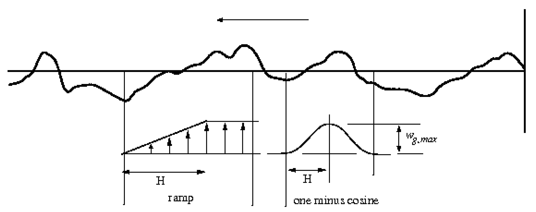
Jones [35] have reviewed the history of gust modeling approaches. Typically, wind gust distributions have two trends: those which can be singled out as discrete gust profiles and those that occur in random pattern (turbulence). The random behaving gusts are described using Fourier’s transform and power spectral density method. Earlier gust studies were limited to fixed and simple discrete gust distributions such as ramp and 1-cosine; these gust profiles are shown in Figure 1. These gusts are characterized by the gust gradient distance (H) and the gust maximum intensity (). According to Jones [35], gust gradient distance is generally assumed to be 100 feet (in the United Kingdom) or 12.5 wing chords (in the United States). A 1-cosine gust profile is described with the following equation:
where is the maximum gust velocity, x is the gust penetration distance, and H denotes the gust gradient distance. The gust penetration distance is time-dependent and depends on the gust-front speed (which equals aircraft speed in this work). For the purposes of this study, is assumed to have a frequency of 1 Hz multiplied by the simulation time.
Though a step gust (sharp edge) is not a realistic gust and is very difficult (if not impossible) to being generated in a wind tunnel, the simulation of this gust gives valuable insight into the general characteristics of the aircraft response to arbitrary gust distributions. Assuming an airplane with quasi-steady aerodynamics and zero vertical motion encounters a sharp edge gust of intensity , the incremental lift coefficient due to the gust is given by Fuller [37] as
where is the lift curve slope, and is the angle of attack in radians due to gust. The vertical acceleration increment, in units of g, due to this gust is
where is the wing loading. According to this equation, the gust loads become important for aircraft with small wing loading and high flying speeds. This led to the first gust load regulations in 1934, which reduced the maneuver load factors in all passenger aircraft to the range of 2.5–4.0 g in order to take into account the incremental load factor when the airplane encounters a gust. Later, a factor of K was added to the sharp-edge gust equation to model the unsteady aerodynamic effects due to gust [37].
The exact unsteady lift response of a flat plate in incompressible flow to a unit step gust was calculated by Hans Georg Küssner [3]. His solution is named Küssner function. The Küssner function can be approximated by an exponential series in the form of [4]:
where is the lift response of the flat plate encountering a step gust, and is the normalized time. The sharp-edge gust hits the plate leading edge at time zero. The lift-gust-curve slope is defined as follows:
In this work, a convolution model is considered to predict linear aerodynamic responses to an arbitrary gust distribution. The model for predicting incremental lift coefficient responses to a gust takes the form of
where is the forcing gust function (i.e., the 1-cosine) as a function of non-dimensionalized time and is the time-dependent lift-gust curve slope due to a sharp-edged gust excitation; can either being replaced with the Küssner approximation function or CFD data from the sharp edge wind gust simulation.
The following steps are to be taken to calculate sharp edge gust response in Cobalt. Steady-state CFD data are first calculated for the calm case (zero gust velocities) at the desired Mach and Reynolds numbers. The gust response is then calculated by imposing a step change in the upward gust velocity at the inflow boundary. The gust will then travel with user-specified gust-front speed from a user-specified initial position outside the gridded domain. The gust travels over the airfoil/aircraft until a solution converges to its new steady conditions. The response function, , is then computed by taking the differences between time-varying responses occurring after encountering the gust and the steady-state solution at calm conditions, and dividing it by the step magnitude of the gust velocity.
3. Flow Solver
The flow solver used for this study is the Cobalt code [38] that solves the unsteady, three-dimensional, and compressible Navier–Stokes equations in an inertial reference frame. In Cobalt, the Navier–Stokes equations are discretized on arbitrary grid topologies using a cell-centered finite volume method. Second-order accuracy in space is achieved using the exact Riemann solver of Gottlieb and Groth [39], and least squares gradient calculations are achieved using QR factorization. To accelerate the solution of the discretized system, a point-implicit method using analytic first-order inviscid and viscous Jacobians is used. A Newtonian sub-iteration method is used to improve the time accuracy of the point-implicit method. Tomaro et al. [40] converted the code from explicit to implicit, enabling Courant–Friedrichs–Lewy (CFL) numbers as high as 10. Some available turbulence models are the Spalart–Allmaras (SA) model [41], the Spalart–Allmaras with rotation/curvature correction (SARC) [41], Wilcox’s k- model [42], and Mentor’s SST (Shear Stress Transport) model [43].
To model an arbitrary wind gust, the “user-defined” boundary condition capability of Cobalt is used. Note that this capability allows gust simulation for any configuration of interest (two- or three-dimensional cases). The user should then provide a subroutine (written in Fortran 90) to treat any boundary condition of the computational grid with customized functions. As an example, in normal (no gust) simulation of the flow around an airfoil, boundary conditions of far-field and no-slip wall available in Cobalt are selected. The far-field conditions of Cobalt use Riemann invariants which enforce the specified flow values at an inflow boundary, but no flow value is enforced at the outflow boundary. For the gust simulation purposes, the far-field boundary condition is replaced with a user-defined one. A subroutine should therefore be provided that defines inflow conditions. The subroutine should have free-stream conditions (Mach, pressure, temperature, etc.) for both the calm and gust conditions. In the calm case, the flow velocity components, pressure, and temperature are specified and are invariant in time. The gust velocities are set to zero as well. These data correspond to the desired Mach and Reynolds numbers. In order to verify the accuracy of scripts, the calm conditions can be compared with normal Cobalt simulations using Riemann invariants at the free-stream. For the similar Mach and Reynolds numbers and flow angles, the user-defined solutions (e.g., integrated forces and moments) should exactly match those calculated using far-field boundary condition.
In the case of a gust, the gust conditions are specified in a time-varying manner appropriate for the type of gust to be modeled, i.e., step-function, cosine, or any arbitrary form. For a step-function gust simulation, the vertical gust component is specified that corresponds to the magnitude of the gust of interest. The gust will travel with user-specified gust-front speed from a user-specified initial position outside the gridded domain. Currently, the gust must start outside of the flow domain to ensure proper gust front formulation. The gust script was originally written by William Strang of Cobalt Solutions, LLC., Springfield, OH, USA, but has been built upon to simulate various gust profiles. Arbitrary gust profiles can be modeled using tabulated data in which gust intensity at different time/positions are listed. In order to assess the scripts, 1-cosine gust profile is considered and is modeled using Equation (1) and tables. The cosine gust is defined by using the number of gust cycles, the frequency of the gust, and the phase. All values in the script are non-dimensionalized using the speed of sound before applying Salas’ farfield boundary condition [44] as well. The position of the gust front during the simulation depends on time and velocity, both of which depend upon where the gust begins and propagates to. Finally, the gust responses using Equation (1) and tabulated data are then compared.
4. Test Cases
4.1. Two-Dimensional NACA0012 Airfoil
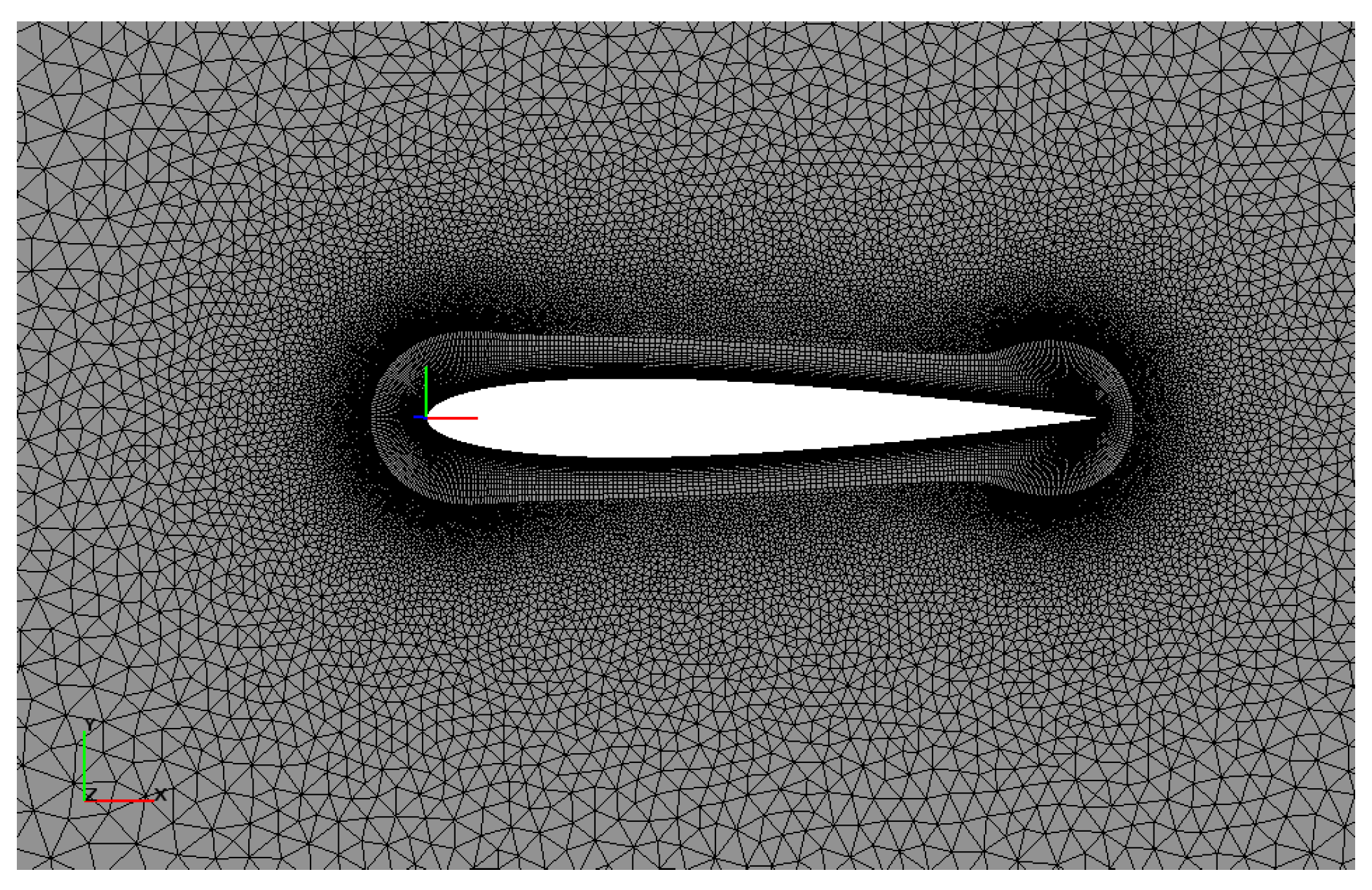
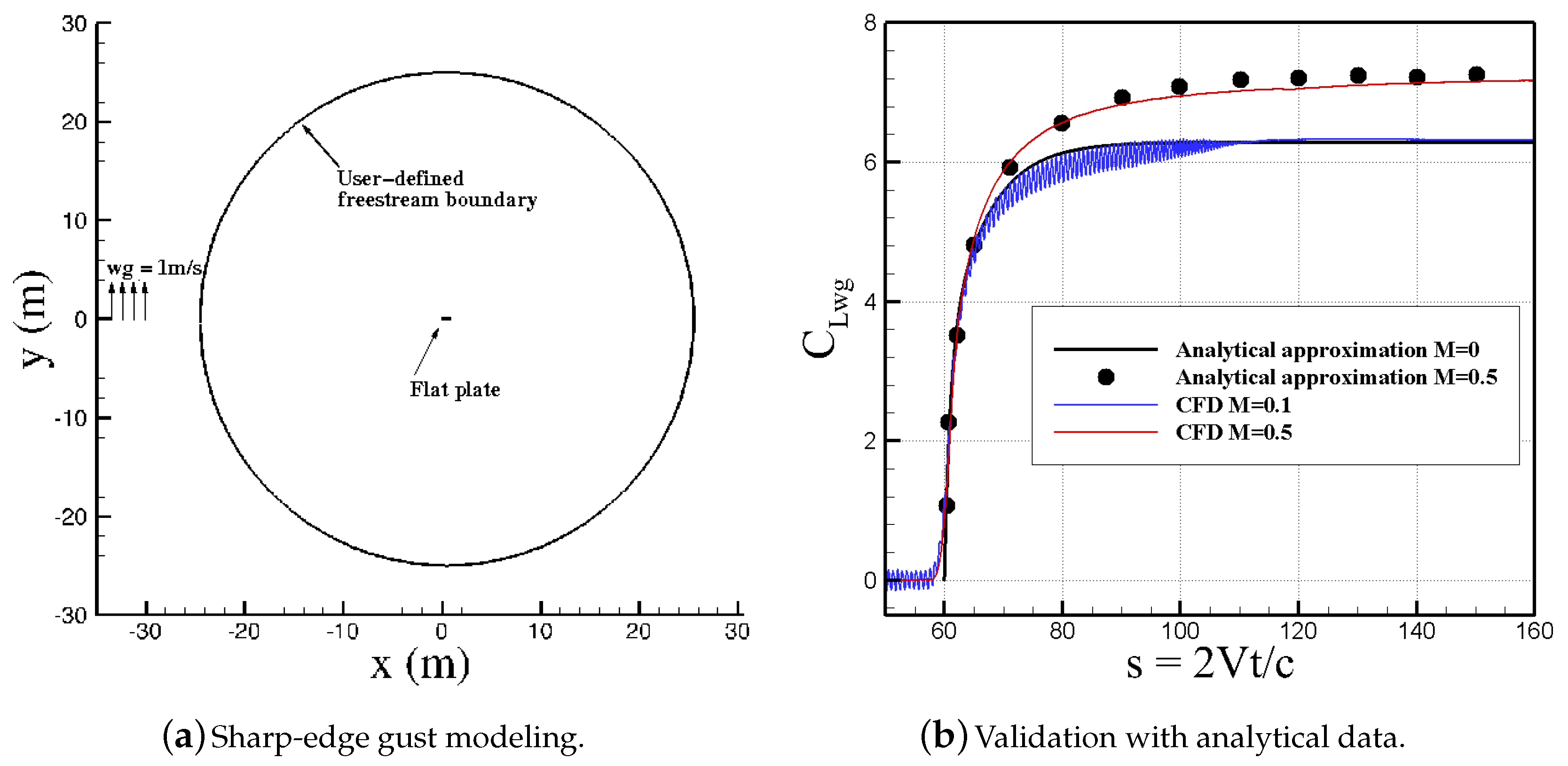
This airfoil is selected because of the available static and dynamic experimental data. The solution of a sharp-edge gust traveling over this airfoil is compared with the Küssner approximation function and might also be compared with a flat plate response. The computational grid of this airfoil was generated using Pointwise. The grid has 72,852 cells with a circular free-stream region with a radius of 50c. The grid cells around the airfoil surface can be seen in Figure 2. Boundary conditions are user-defined for the free-stream, and no-slip wall for the airfoil. The chord length of the NACA0012 airfoil is 1 m. The pitch axis and moment reference point is 0.25 m past the leading edge.
The computational grid had been previously validated with static and dynamic experimental data in [27]. The Spalart–Allamaras turbulence model is used for all two-dimensional simulations.
4.2. The HIRENASD Model
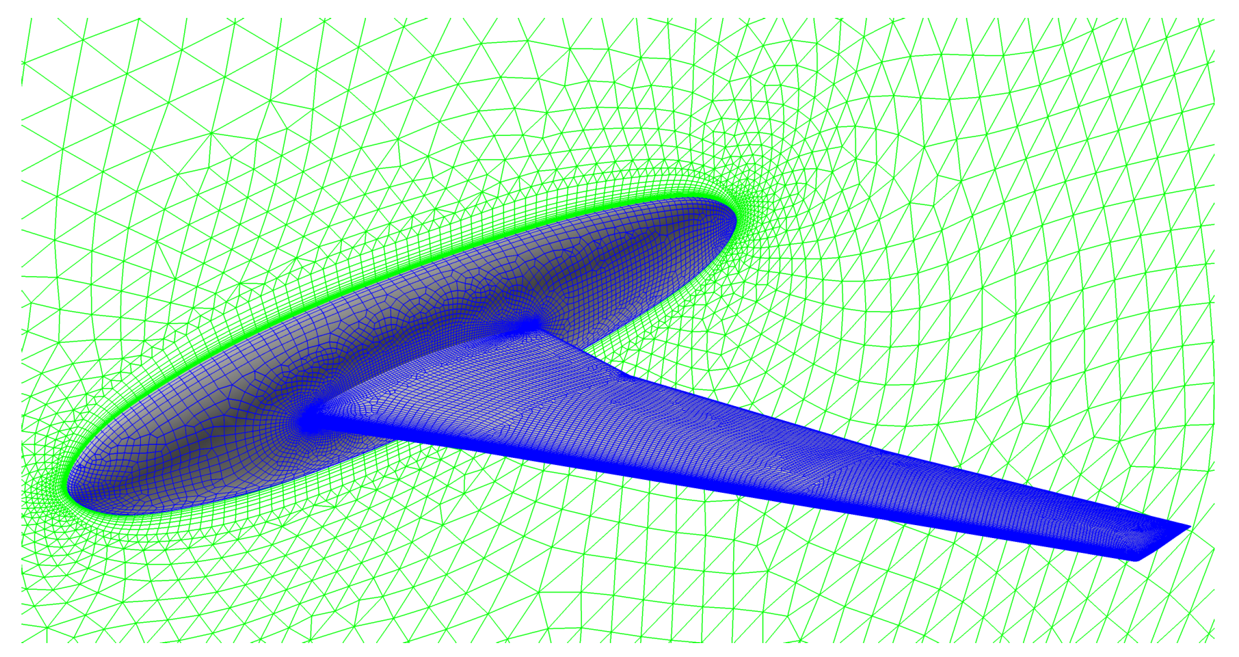
After the two-dimensional testing were completed, a three-dimensional test case was chosen to be accomplished using the HIRENASD configuration, a configuration funded by the German Aerospace Center (DLR) [32]. The HIRENASD configuration resembles a typical large passenger transport aircraft wing with a leading sweep angle of 34 with a supercritical wing profile of BAC 3-11. The wind tunnel model has a half span of 1.28571 m, a mean aerodynamic chord of 0.3445 m, and a wing reference area of 0.3925 m. The computational grid used can be seen in Figure 3 and has approximately 4 million cells. The Spalart–Allmaras with the rotational correction (SARC) turbulence model was selected for the three-dimensional computational case tested.
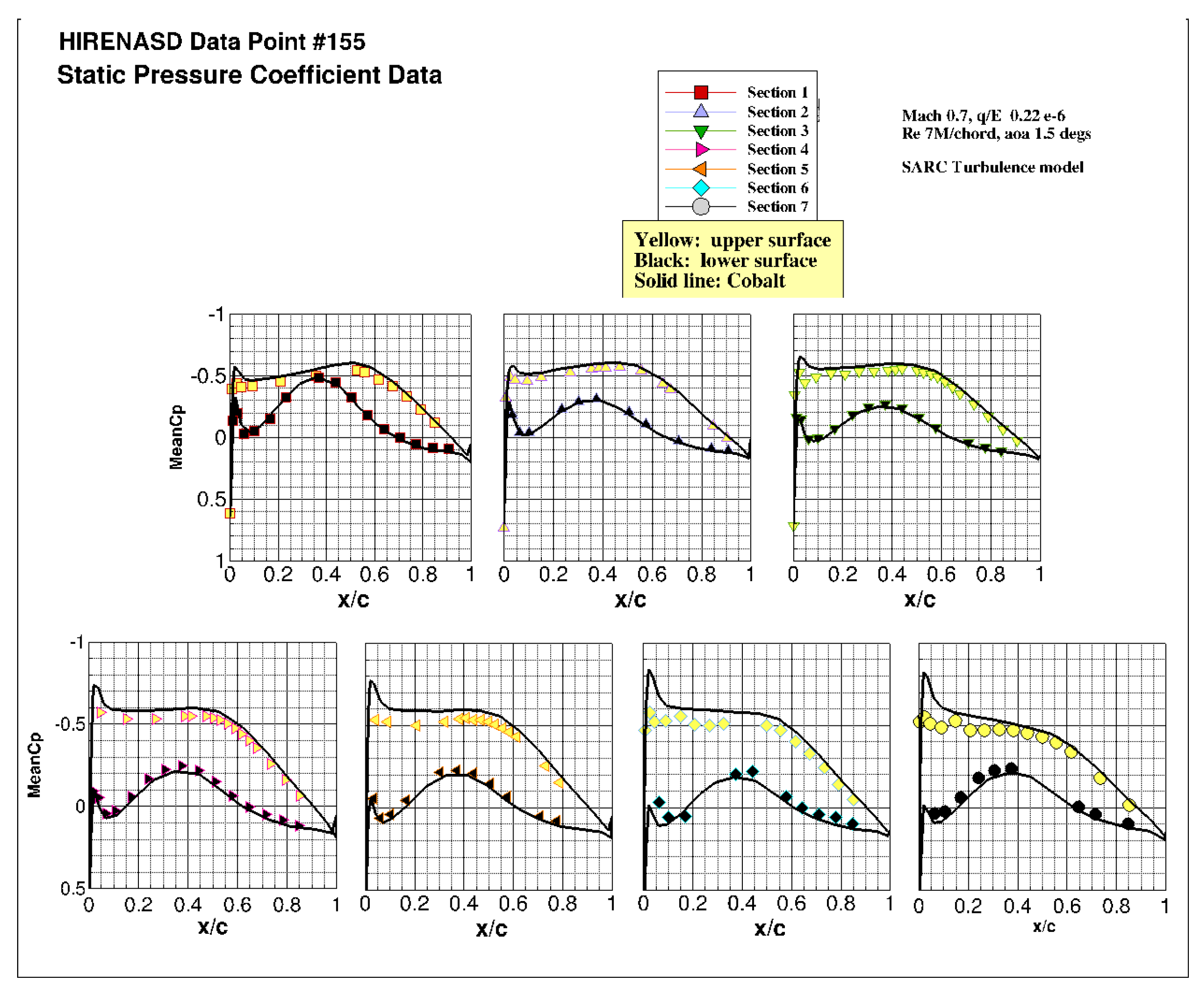
Experimental data of the HIRENASD configuration is available from the European Transonic Wind tunnel (ETW), which is a cryogenic facility with a closed circuit with nitrogen gas as a fluid. The measurements include a pressure coefficient data at different span wise positions given in [32]. These measurements correspond to Mach 0.7 and a Reynolds per length of 7 million and is considered in this work as validation for the computational results.
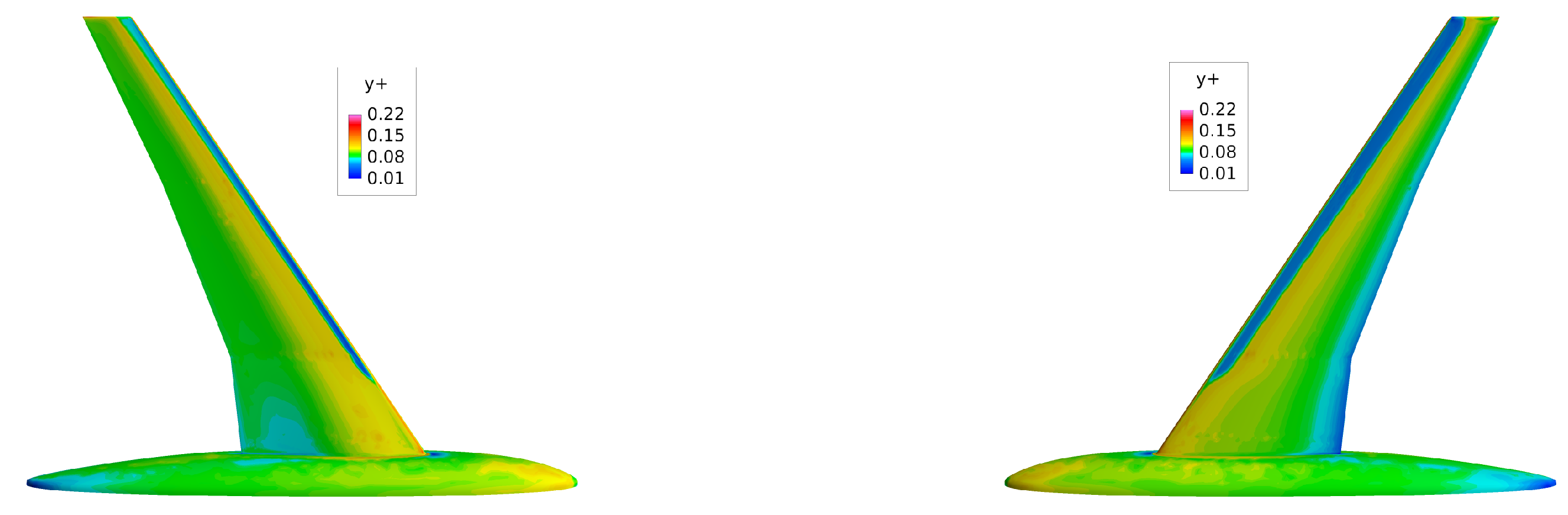
A viscous grid is generated around this configuration. The grid has three boundary conditions: far-field, symmetry, and no-slip wall. The grid is shown in Figure 3 has prism layers around the walls and tetrahedra cells elsewhere. This grid has around 4 million cells. Figure 4 shows the grid calculated values at the upper and lower surfaces at Mach 0.7. Figure 5 compares Cobalt predictions of pressure coefficient data with experimental data measured at tap positions. The simulations use the SARC turbulence model and run for Mach 0.7, a Reynolds per length of 7 million, and an angle of attack of 1.5. Figure 5 shows that the CFD data agree well with the experimental data at most locations, in particular at the lower surfaces. The biggest discrepancy is seen at the upper surface, at positions near the wing tip, and at the wing’s leading edge, where CFD predictions over-estimate experimental pressure data. Note that, in simulations, the body is rigid, while this is considered a flexible model in the wind tunnel. Overall, these results confirm the validity and accuracy of computational methods used in this work for the HIRENASD configuration and any further results using this configuration.
5. Results and Discussions
Computational resources were provided by the DoD’s High Performance Computing Modernization Program. All airfoil simulations are run on the U.S. Air Force Research Laboratory (AFRL) ‘Lightning’ Cray XC30 system (2370 computing nodes with 24 cores per node running two Intel Xeon E5-2697v2 processors at a base core speed of 2.7 GHz with 63 GBytes of RAM available per node). HIRENASD simulations were run on the Engineering Research Development Center’s (ERDC’s) ‘Topaz’ SGI ICE X System (3456 computing nodes with 36 cores per node running two Intel Xeon E5-2699v3 processors at a base core speed of 2.3 GHz with 117 GBytes of RAM available per node). All gust simulations resumed from a calm condition solved with 2500 time steps to allow the flow around the vehicle to become steady. Second-order accuracy in time and three Newton sub-iterations are used as well. NACA0012 airfoil simulations used SA turbulence model and a time step of 1 × s, while the HIRENASD configuration used the SARC turbulence model and a time step of 1 × s.
5.1. Validation and Verification of User-Defined Codes
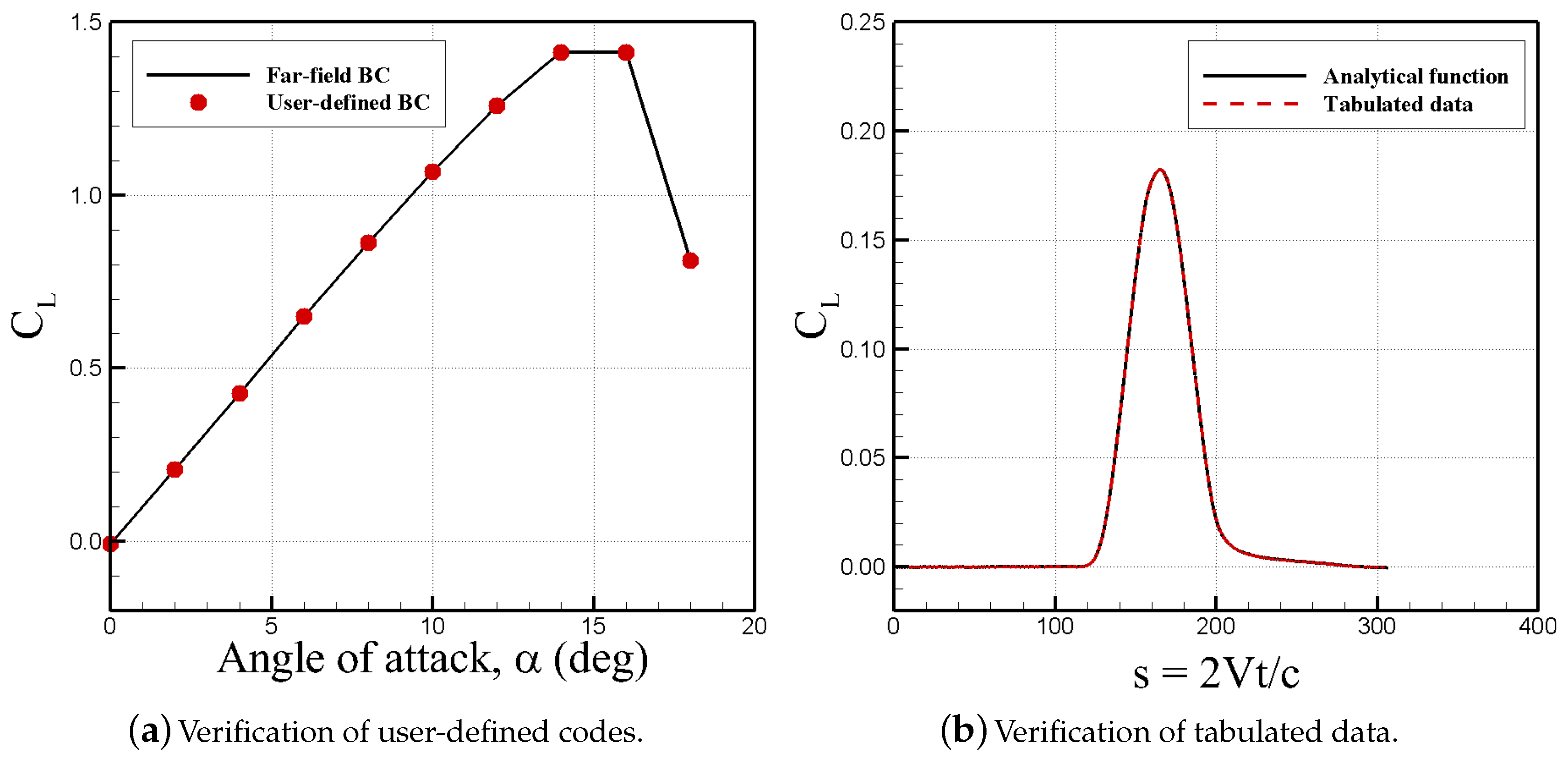
The first set of results presents the verification plots for the codes developed by the authors. In Cobalt, the free-stream region is modeled with Riemann invariants that are integrated into the solver. In this work, however, the free-stream boundary of the computational grid is represented by a user-defined code. This code was scripted for modeling calm and gust simulations over any arbitrary configuration. In order to verify the scripts, Figure 6a shows the lift coefficient of NACA0012 airfoil calculated from (1) the far-field boundary condition (2) and the user-defined codes run for calm conditions. In the first method, the free-stream angle of attack, Mach number, pressure, and temperature are defined in the Cobalt main input file. Simulations shown in Figure 6a correspond to Mach number of 0.1 and the static pressure and temperature values in order to have a Reynolds number of 5.93 × 10. The angle of attack changes from zero to 20. In the second method, the free-stream data of the main input file are discarded; instead, they are given in the user-developed script. Flow velocity components are specified to have a Mach number of 0.1 and an angle of attack in the range of zero to 20. Static pressure and temperature are defined to have a Reynolds number of 5.93 × 10. For the calm conditions, gust velocities are set to zero as well. Figure 6a shows that the calculated lift coefficient values from the used-defined code perfectly match with those obtained from simulations using the far-field boundary condition.
For modeling an arbitrary gust distribution, the script written by the authors defines the gust data in tabular format. The table consists of gust velocity values at specific time instants. Figure 6b shows NACA0012 airfoil lift coefficient responses against a 1-cosine gust profile. The responses are from (1) an analytical function scripted and (2) tabulated data of the 1-cosine function. The gust profile has one cycle, amplitude of 1 m/s, and a gradient distance (H) of about 17c. Figure 6b shows that solutions from both methods of defining the gust perfectly match, confirming the capability of the code to model any gust profile. Notice that, in Figure 6b, gust should travel 60 m with a speed of about 34 m/s before it hits the airfoil leading edge. One cost associated with modeling wind gusts with imposing the gust velocities at the inflow boundary is the computational costs needed to propagate the wind across the flow domain until it has interacted with the object.
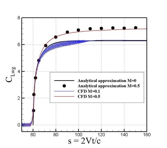
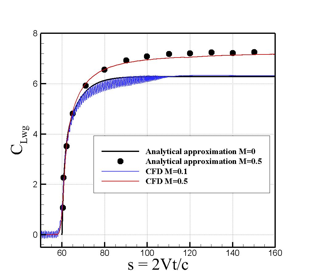
Finally, the sharp-edge predictions from Cobalt at inflow Mach numbers of 0.1 and 0.5 are compared with analytical solutions of a thin airfoil at zero Mach number and Mach 0.5 in Figure 7. In both runs, the gust velocity is 1 m/s, and the gust travels from . Analytical approximation data correspond to Jones [4] for zero Mach number and Mazelsky and Drischle [5] for . In order to have a fair comparison, a flat plate of 1 m long was modeled in the solver. The computational domain has a circular free-stream around the plate with a radius of 25 m as shown in Figure 7a.
Overall, the calculated CFD trends and values (normalized by gust intensity and free-stream velocity) match very well with analytical solutions. However, CFD simulations at Mach 0.1 show oscillating behavior as the gust approaches the plate and crosses over it. This is possibly due to the strong interactions between the plate and the gust at small Mach numbers or the large ratios of gust to free-stream velocity. Another interesting observation is that the analytical solutions show zero lift increment until the time that gust hits the most forward point of the plate. In contrast, CFD lift data begin to rise before the gust hits the plate. Figure 7 shows that the sharp edge responses reach different steady-state values depending on the Mach number; this value increases by increasing the Mach number due to compressibility effects. In addition, the response trend shows a longer transient behavior to reach its steady-state value than .
5.2. Simulation Results of NACA0012 Airfoil
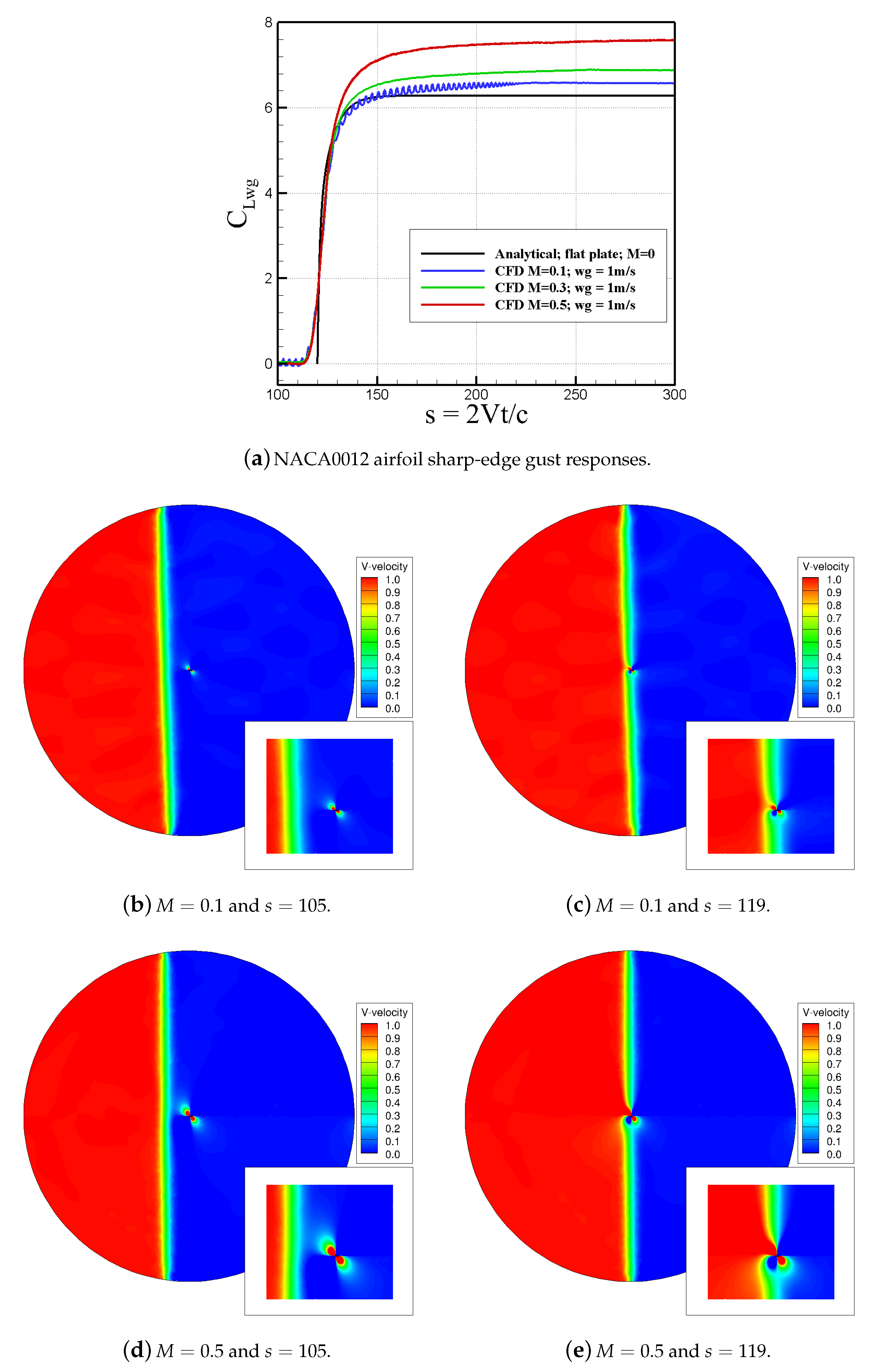
Firstly, the NACA0012 airfoil was used to simulate unit sharp edge gust responses across the flow domain for Mach numbers 0.1, 0.3, and 0.5. The calculated (lift-gust curve slope) values at these Mach numbers can be seen in Figure 8 and are shown with the analytical approximation function at a zero Mach number. Figure 8 shows that the airfoil response at does not match with the analytical solution as it is valid only for thin airfoils. The responses reach larger steady-state values, as the Mach number increases due to compressibility effects. In addition, Figure 8 shows that the gust effects on airfoil could be seen even before the gust hits the airfoil leading edge. Oscillating behavior could be seen for the airfoil response at as well.
Figure 8b–e show the flow solutions of a unit sharp edge gust traveling over the airfoil at a Mach number of 0.1 and 0.5. In these figures, gust travels from left to right. Inspecting velocity data shows that the sharp edge gust is not a very exact representative of the mathematical model because there is no visible gust front where, at its right side, vertical velocity is zero and then becomes 1 m/s. Instead, the vertical velocity changes from zero to 1 m/s over a small distance. Note that modeling an exact sharp edge in CFD is not possible because of discontinuity in the flow field. This might explain why airfoil responds sooner to gusts than do analytical solutions. Additionally, Figure 8b–e show that the gust profile will be affected as it approaches and crosses over the airfoil. However, the interaction time between airfoil and gust is much shorter for larger Mach numbers. These interactions cause the oscillation behavior seen at small Mach number plots.
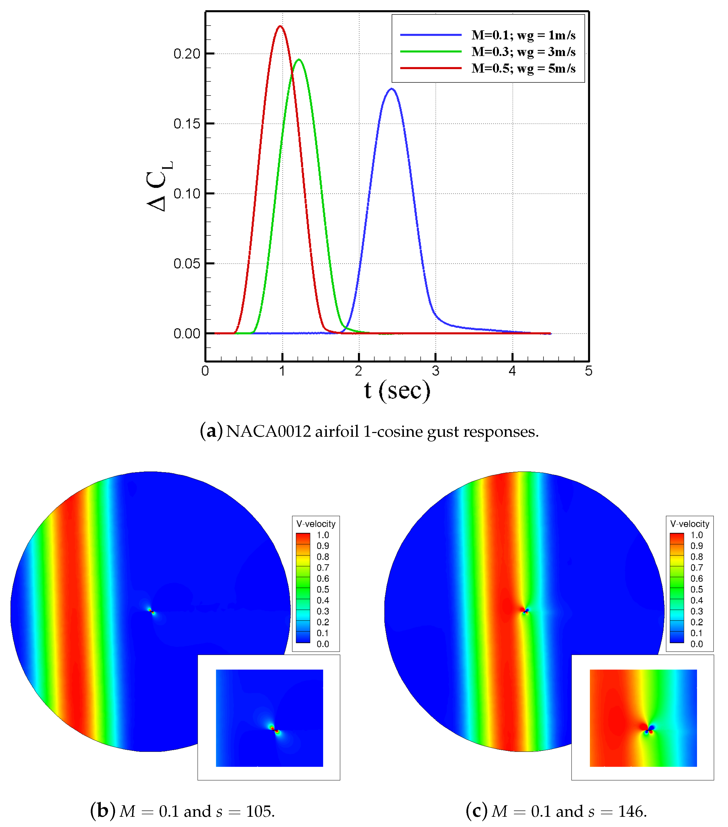
Figure 9 shows 1-cosine gust responses using an analytical equation. Figure 9a presents lift coefficient increments from calm conditions, , for Mach numbers 0.1, 0.3, and 0.5 at wind gust speeds of 1 m/s, 3 m/s, and 5 m/s, respectively. In all simulations, the gust front travels from , which is outside the inflow boundary towards the airfoil with free-stream velocity, V, at a zero angle of attack. Though is similar in these runs, but the increments are bigger for larger Mach number again due to compressibility effects. Notice that gust hits the airfoil at different times because of different gust front speeds, such that the larger the Mach number is, the sooner the gust impacts the airfoil. Figure 9b–c show the wind gust as it propagates over the flow domain until it reaches the airfoil. The vertical velocity data show the 1-cosine gust profile with a centered maximum velocity. Figure 9c shows that gust profile changes due to its interaction with the airfoil flow field.
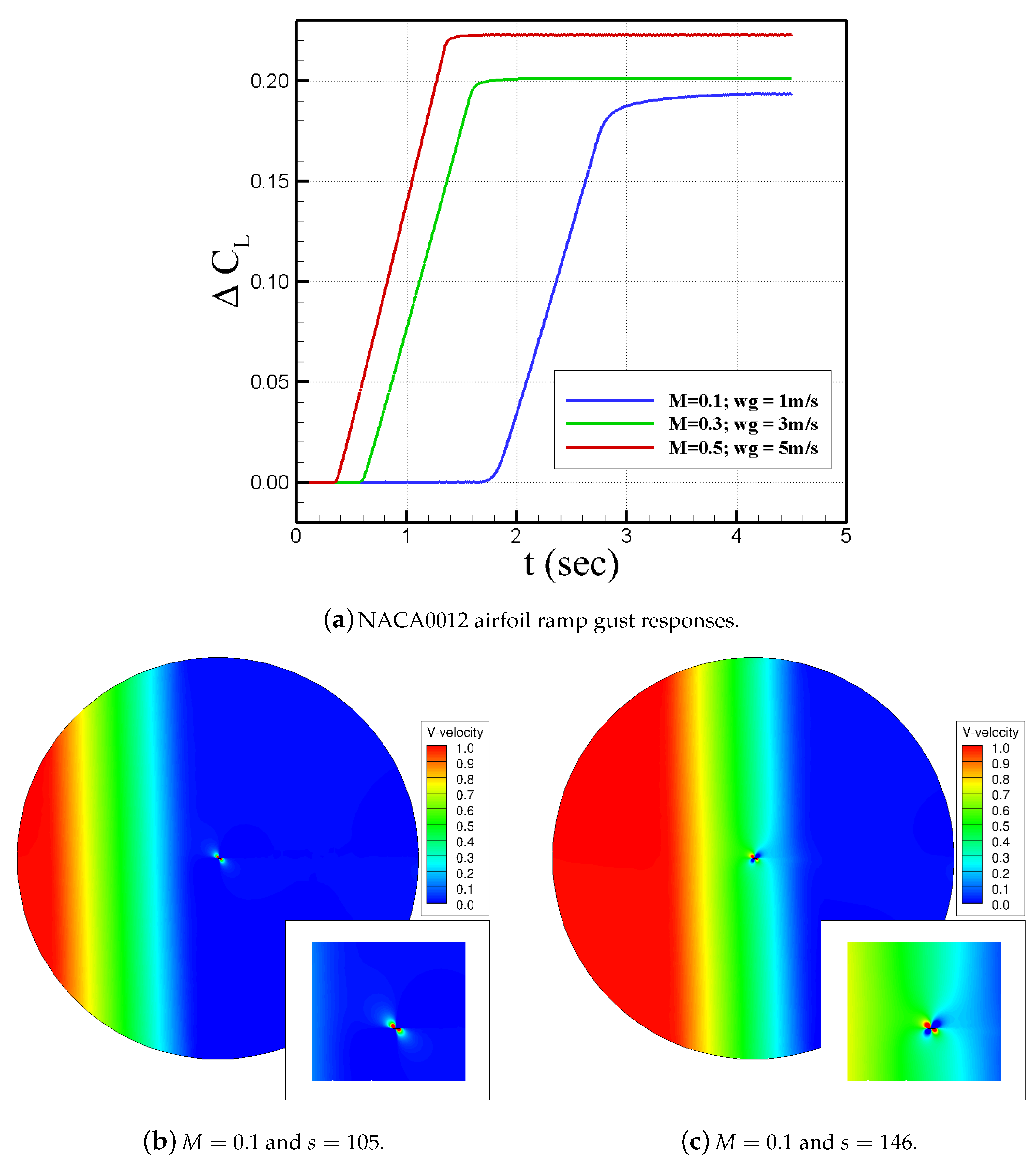
The ramp gusts can be seen in Figure 10, with Figure 10a displaying the (lift coefficient increments from calm conditions) for Mach numbers 0.1, 0.3, and 0.5 at wind gust speeds of 1 m/s, 3 m/s, and 5 m/s, respectively. In Figure 10b–c, the ramp wind gust is seen to propagate nicely over the flow domain until it reaches the airfoil.
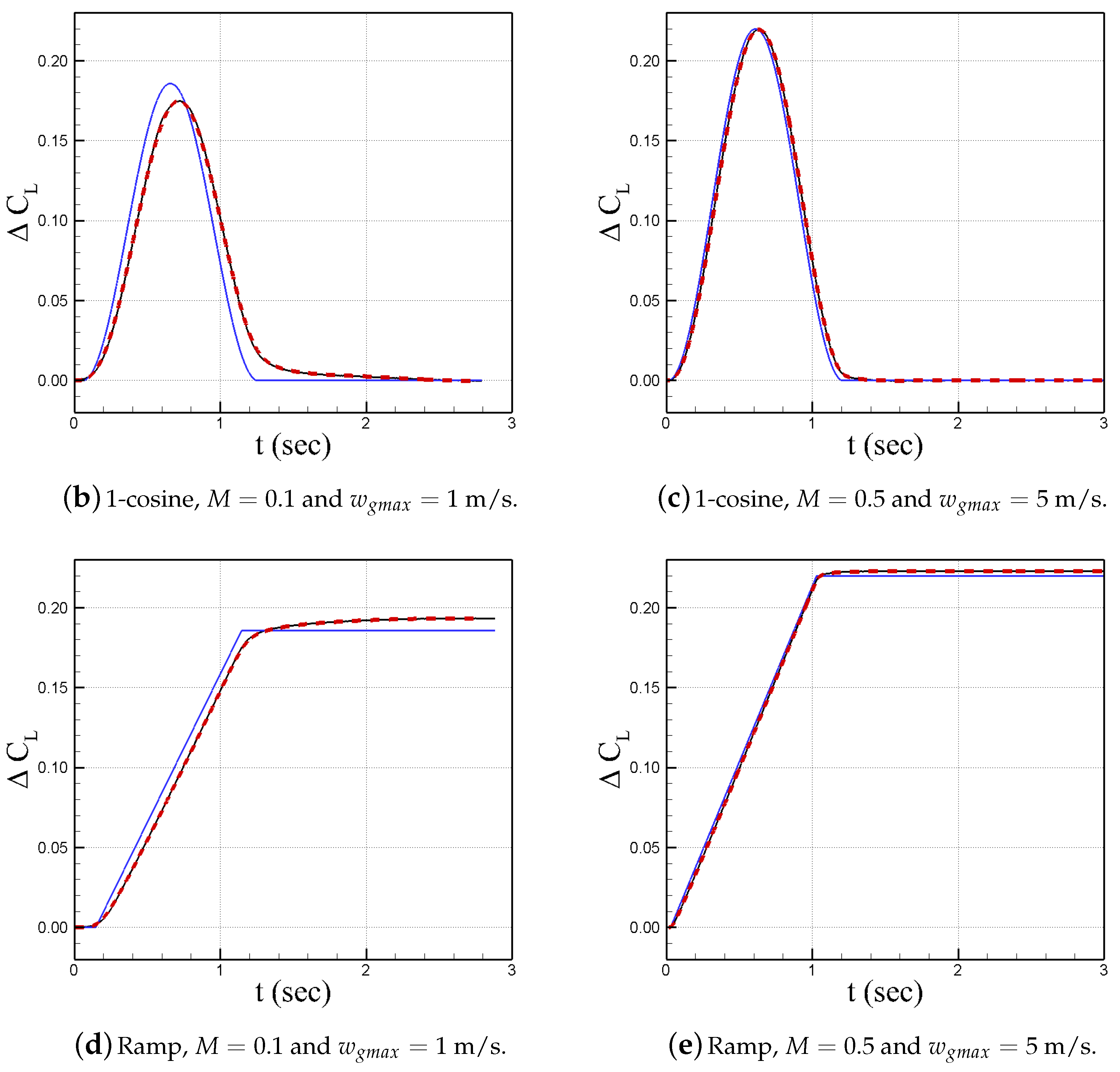
Plotted in Figure 11 is the CFD simulation data, the quasi-steady model using Equation (2), and the convolution model (6) for both cosine and ramp gust shapes. The convolution model is able to use the sharp edge gust simulation results, and its predictions perfectly match with the CFD data obtained from Cobalt, matching the peak magnitude, shape, phase (with respect to the wind gust), and transient effects towards the end. The quasi-steady model is able to approximate everything but is not nearly as accurate. It lacks phase correction, accurate magnitudes, and transient effects such that the smaller the Mach number, the more poorly matches the CFD or convolution model data.
5.3. Simulation Results of HIRENASD Configuration
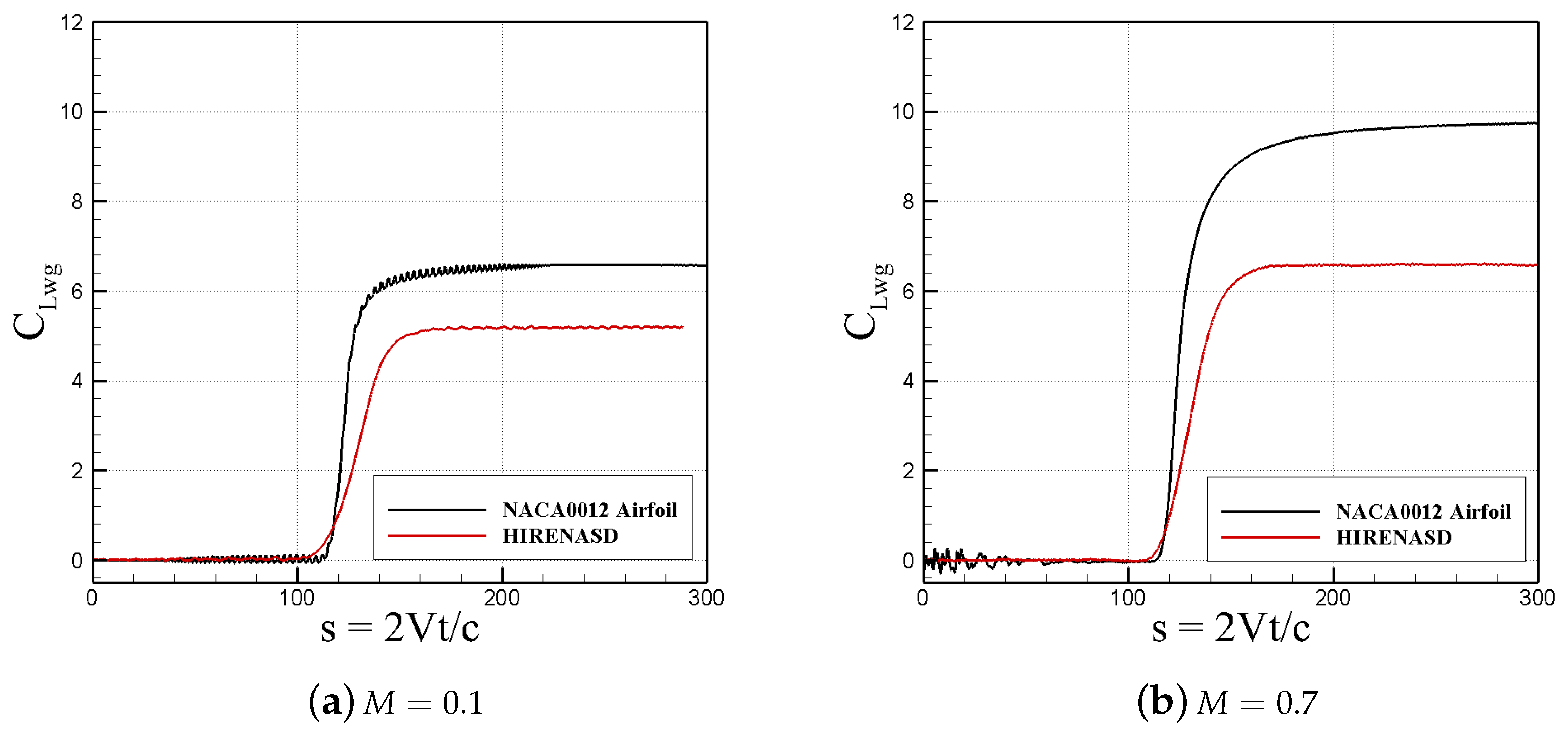
The HIRENASD configuration underwent test environments similar to those that of the NACA0012 simulations. At Mach numbers of 0.1 and 0.7 and a wind gust of 1 m/s, a unit sharp edge gust was tested, and the (lift-gust curve slope) can be seen in Figure 12, where the result is shown with those of the NACA0012 simulations. The HIRENASD gust begins from and the geometry has a mean aerodynamic chord different from that of the airfoil. The HIRENASD plots in Figure 12 are therefore translated to match the starting point of the NACA0012 airfoil. Figure 12 shows that the HIRENASD indicial response trends are very different from those of the NACA0012 airfoil. Interestingly, it has a shorter build-up time to a steady-state solution. Note that the steady-state values are lower than those found for the airfoil due to wing tip losses and other effects. The only method to estimate 3D aircraft responses is CFD, since analytical solutions are not applicable and it is not feasible to test a sharp edge gust in a wind tunnel.
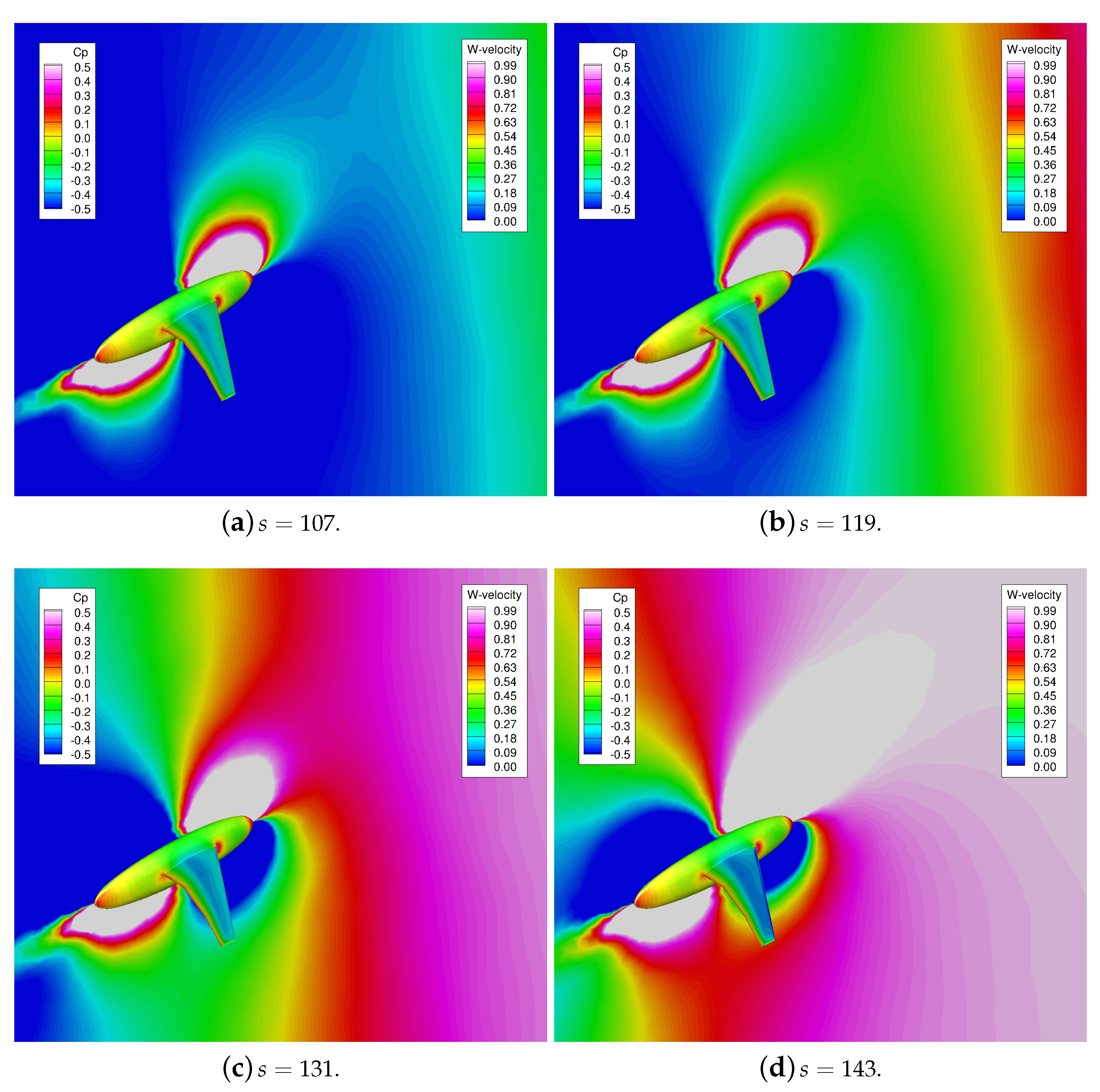
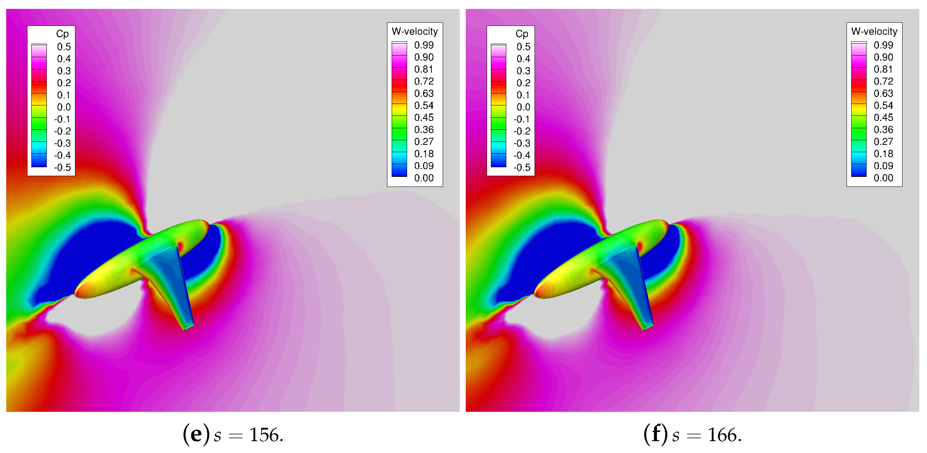
In more detail, Figure 13 depicts a sharp edge gust flowing across the flow domain on the HIRENASD configuration. The vertical velocity is depicted on the symmetry plane, and the pressure coefficient is presented on the HIRENASD geometry. In each successive subplot, the gust is seen propagating from right to left until it has almost made complete contact in Figure 13c,d and reaches a steady-state value by Figure 13f. The gust shape again changes as it interacts with the vehicle. The wing upper surface shows pressure changes as the gust crosses over it.
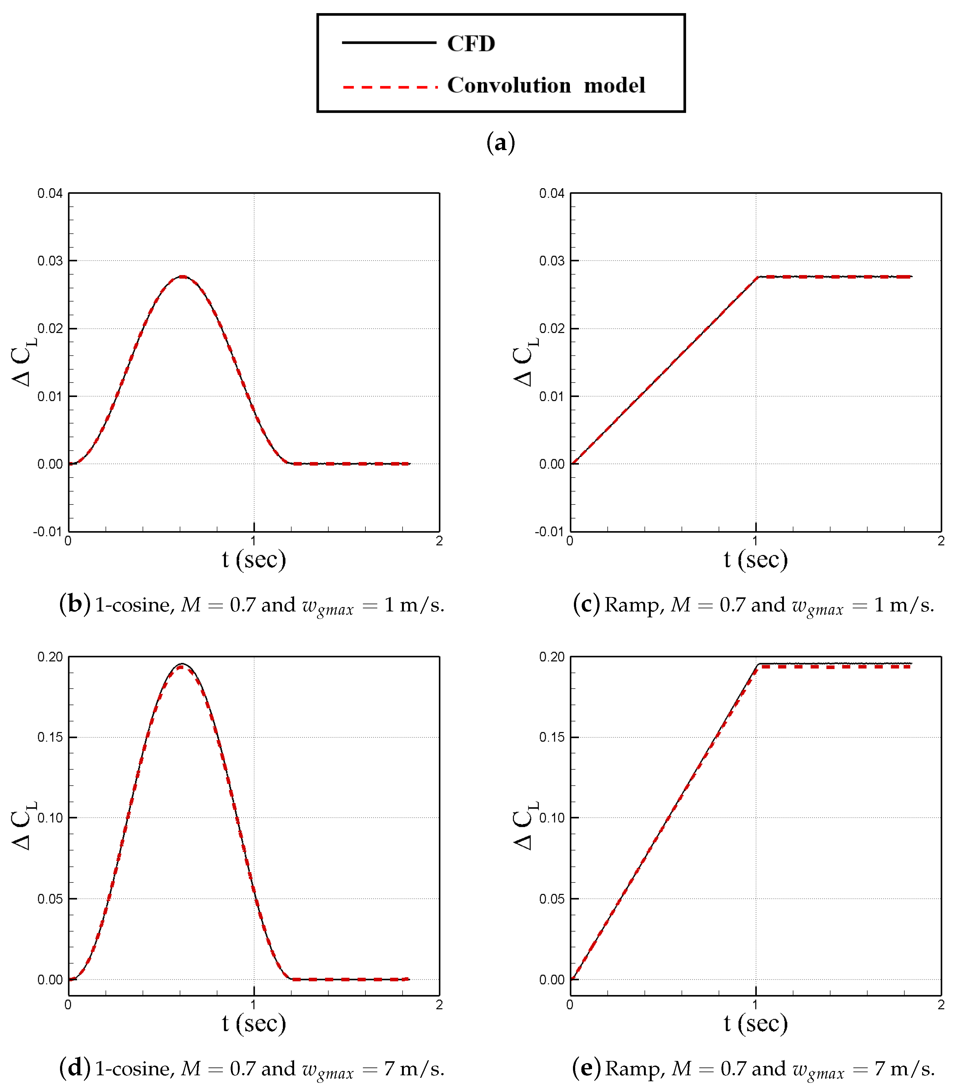
Additionally, 1-cosine and ramp wind gusts are tested at Mach 0.7 with upward wind gusts of 1 m/s and 7 m/s coming from the inflow boundary at . The results of the CFD predictions are shown in Figure 14, where the trends of caused by the cosine and ramp simulations appear to reacting similarly to how the NACA0012 simulations did. The convolution model is also applied by using the data from the sharp edge gusts to predict the cosine and ramp gusts at Mach 0.7 with wind gust speeds of 1 m/s and 7 m/s. The results show that the model is able to accurately predict time-accurate simulation data, as seen in Figure 14b–e.
5.4. Computational Costs
Running a simulation where the wind gust has to start outside of the flow domain and propagate across until it reaches the vehicle can become computationally costly. For the flat plate example, the sharp edge gust propagates from outside its domain with at zero time. The gust front speed was set to free-stream speed. Figure 7 shows that CFD prediction matches with the analytical approximation data. There is a “time-to-hit-gust” in the CFD data; the data obtained during this time are not of any significant importance in this work.
For the NACA0012 airfoil at M = 0.1, a starting gust position x = , and a time step of 1 × 10 s, it takes approximately 17,632 time steps in Cobalt for the gust front to reach x = 0, which is the location of the leading edge of the airfoil. The computational cost is inversely proportional to both the size of the domain and the Mach number of the flow field being investigated. The computational cost increases as the size of the object increases and the size of the gust increases in order to obtain a complete representation of flow features that develop after the gust has passed and reached steady-state values.
However, in order to remain consistent in making scripts and handling data, 2500 startup (zero gust speed) iterations followed by 47,500 simulation time steps were chosen for the two-dimensional NACA0012 cases. This design choice led to simulations using approximately 1.5 CPU hours (a few minutes on 24 cores) for the startup iterations and 50–72 CPU hours ( 2.5 h of real time on 24 cores) for the wind gust simulations. The total CPU hour usage for the 2D portion of this study to obtain sharp edge gust and cosine simulation data was approximately 2952 CPU hours on the “Lightning” system, but this did not include the CPU time used in diagnosing errors or ramp simulations. The cost of creating ROM was only 246 CPU hours.
The 3D HIRENASD simulation took significantly more processing power to run a single simulation due to the increased number of elements. In obtaining the results, 2500 startup iterations used approximately 1500 CPU hours, and the remaining 15,000 iterations to obtain the wind gust simulation data used approximately 8300 CPU hours (4 hours of wall clock time on 2016 cores) for a total of 19,600 CPU hours used on the ’Topaz’ system to calculate the sharp edge and cosine gust simulations, and this does not include the CPU time used in diagnosing errors. This particular case could net a total of 50% savings or more, i.e., 9800+ CPU hours, if the sharp edge gust only were calculated and if the convolution model were applied to obtain the cosine gust.
6. Conclusions
A user-defined script written for Cobalt was developed and used to model wind gusts by forming them at the far-field boundary and allowing them to propagate across the flow domain. The script was proven to offer no difference in answers calculated by traditional methods of running Cobalt simulations. Sharp edge, ramp, and cosine gusts can now be modeled using Cobalt, offering enough precision to match calculations from other works and analytical solutions.
By using a sharp edge gust and the convolution model, the coefficient of lift was estimated and matched to a cosine gust simulated in Cobalt. The convolution model was found to be as accurate as the simulations themselves and would finish calculations on the order of a minute or two compared to the many CPU hours needed in finding a solution with Cobalt.
Acknowledgments
This article was approved for Public Release with Distribution A. This material is based in part on research sponsored by the US Air Force Academy under agreement number FA7000-17-2-0007. The U.S. Government is authorized to reproduce and distribute reprints for governmental purposes notwithstanding any copyright notation thereon. The views and conclusions contained herein are those of the authors and should not be interpreted as necessarily representing the official policies or endorsements, either expressed or implied, of the organizations involved with this research or the U.S. Government. The authors would like to thank William Strang of Cobalt Solutions, LLC., in Springfield, Ohio, for giving us a script to model wind gusts in the Cobalt flow solver. The numerical simulations have been performed on the HPCMP’s Topaz cluster located at the ERDC DoD Supercomputing Resource Center (DSRC) and the Air Force Research Laboratory (AFRL) Lightning cluster.
Author Contributions
Mehdi Ghoreyshi and Ivan Greisz run simulations, generated all plots, and prepared this article. Adam Jirasek generated the computational grids and provided a script to model gust profiles using tabulated data. Matthew Satchell is the program manager of this research at USAFA.
Conflicts of Interest
The authors declare no conflict of interest.
Nomenclature
| a | acoustic speed, m s |
| c | chord length |
| CFD | computational fluid dynamics |
| CPU | central processing unit |
| lift coefficient | |
| lift curve slope | |
| lift-gust curve slope | |
| pressure coefficient, | |
| CREATE | Computational Research and Engineering Acquisition Tools and Environments |
| DDES | Delayed Detached Eddy Simulation |
| DoD | Department of Defense |
| ETW | European Transonic Windtunnel |
| H | gust gradient distance, m |
| HIRENASD | high Reynolds number aero-structural dynamics |
| HPC | High Performance Computing |
| incremental lift | |
| M | Mach number, V/a |
| vertical acceleration increment | |
| p | static pressure, N/m |
| free-stream pressure, N/m | |
| Küssner exponential series approximation or sharp edge gust data | |
| free-stream dynamic pressure, N/m | |
| s | normalized time |
| S | wing area |
| SA | Spalart–Allmaras |
| SARC | Spalart–Allmaras with rotational and curvature correction |
| RANS | Reynolds Averaged Navier Stokes |
| t | time, s |
| USAFA | United States Air Force Academy |
| free-stream velocity, m s | |
| u,v,w | velocity components, m s |
| gust vertical velocity, m s | |
| maximum gust vertical velocity, m s | |
| X | gust penetration distance, m |
| x,y,z | grid coordinates, m |
| non-dimensional wall normal distance |
References
- Bennett, R.M.; Gilman, J., Jr. A Wind-Tunnel Technique for Measuring Frequency-Response Functions for Gust Load Analyses. J. Aircr. 1966, 3, 535–540. [Google Scholar] [CrossRef]
- Noback, R. Comparison of Discrete and Continuous Gust Methods for Airplane Design Loads Determination. J. Aircr. 1986, 23, 226–231. [Google Scholar] [CrossRef]
- Küssner, H.G. Zusammenfassender Bericht über den instationären Auftrieb von Flügeln. Luftfahrtforschung 1936, 13, 410–424. [Google Scholar]
- Jones, R.T. The Unsteady Lift of a Wing of Finite Aspect Ratio; Technical Report; National Advisory Committee for Aeronautics: Langley Field, VA, USA, 1940.
- Mazelsky, B.; Drischler, J.A. Numerical Determination of Indicial Lift and Moment Functions for a Two-Dimensional Sinking and Pitching Airfoil at Mach Numbers 0.5 and 0.6; Technical Report; National Advisory Committee for Aeronautics: Langley Field, VA, USA, 1952.
- Von Karman, T.; Sears, W.R. Airfoil Theory for Non-Uniform Motion. J. Aeronaut. Sci. 1938, 5, 379–390. [Google Scholar] [CrossRef]
- Hakkinen, R.J.; Richardson, A.S., Jr. Theoretical and Experimental Investigation of Random Gust Loads Part I: Aerodynamic Transfer Function of a Simple Wing Configuration in Incompressible Flow; Technical Report; National Advisory Committee for Aeronautics Report; National Advisory Committee for Aeronautics: Washington, DC, USA, 1957.
- Comte-Bellot, G.; Corrsin, S. The Use of a Contraction to Improve the Isotropy of Grid-Generated Turbulence. J. Fluid Mech. 1966, 25, 657–682. [Google Scholar] [CrossRef]
- Roadman, J.; Mohseni, K. Gust Characterization and Generation for Wind Tunnel Testing of Micro Aerial Vehicles; AIAA Paper 2009-1290; AIAA: Reston, VA, USA, 2009. [Google Scholar]
- Valente, C.; Lemmens, Y.; Wales, C.; Jones, D.; Gaitonde, A.; Cooper, J.E. A Doublet-Lattice Method Correction Approach for High Fidelity Gust Loads Analysis; AIAA Paper 2017-0632; AIAA: Reston, VA, USA, 2017. [Google Scholar]
- Weishäupl, C.; Laschka, B. Euler Solutions for Airfoils in Inhomogeneous Atmospheric Flows. J. Aircr. 2001, 38, 257–265. [Google Scholar]
- Heinrich, R.; Reimer, L. Comparison of Different Approaches for Gust Modeling in the CFD Code TAU. In Proceedings of the International Forum on Aeroelasticity and Structural Dynamics, Bristiol, UK, 24–26 June 2013. [Google Scholar]
- Jirasek, A. CFD Analysis of Gust Using Two Different Gust Models. In Proceedings of the RTO AVT-189 Specialists’ Meeting on Assessment of Stability and Control Prediction Methods for Air and Sea Vehicles, Portsmouth, UK, 12–14 October 2011. [Google Scholar]
- Raveh, D.E.; Zaide, A. Numerical Simulation and Reduced-Order Modeling of Airfoil Gust Response. AIAA J. 2006, 44, 1826–1834. [Google Scholar] [CrossRef]
- Wales, C.; Jones, D.; Gaitonde, A. Prescribed Velocity Method for Simulation of Aerofoil Gust Responses. J. Aircr. 2014, 52, 64–76. [Google Scholar] [CrossRef]
- Da Ronch, A.; Tantaroudas, N.D.; Badcock, K.J. Reduction of Nonlinear Models for Control Applications; AIAA Paper 2013-1491; AIAA: Reston, VA, USA, 2013. [Google Scholar]
- Singh, R.; Baeder, J.D. Direct Calculation of Three-Dimensional Indicial Lift Response Using Computational Fluid Dynamics. J. Aircr. 1997, 34, 465–471. [Google Scholar] [CrossRef]
- Förster, M.; Breitsamter, C. Aeroelastic Prediction of Discrete Gust Loads Using Nonlinear and Time-Linearized CFD-Methods. J. Aeroelast. Struct. Dyn. 2015, 3, 19–38. [Google Scholar]
- Bartels, R.E. Development, Verification and Use of Gust Modeling in the NASA Computational Fluid Dynamics Code FUN3D; AIAA Paper 2013-3044; AIAA: Reston, VA, USA, June 2013. [Google Scholar]
- Siegel, S.; Cohen, K.; McLaughlin, T. Feedback Control of a Circular Cylinder Wake in Experiment and Simulation; AIAA Paper 2003-3569; AIAA: Reston, VA, USA, 2003. [Google Scholar]
- Bergeron, K.; Cassez, J.F.; Bury, Y. Computational Investigation of the Upsweep Flow Field for a Simplified C-130 Shape; AIAA Paper 2009-0090; AIAA: Reston, VA, USA, 2009. [Google Scholar]
- Ghoreyshi, M.; Jirasek, A.; Cummings, R.M. CFD Modeling for Trajectory Predictions of a Generic Fighter Configuration; AIAA Paper 2011-6523; AIAA: Reston, VA, USA, 2011. [Google Scholar]
- Ghoreyshi, M.; Jirasek, A.; Cummings, R.M. Closed Loop Flow Control of a Tangent Ogive at a High Angle of Attack; AIAA Paper 2013-0395; AIAA: Reston, VA, USA, 2013. [Google Scholar]
- Ghoreyshi, M.; Bergeron, K.; Seidel, J.; Jirasek, A.; Lofthouse, A.J.; Cummings, R.M. Prediction of Aerodynamic Characteristics of Ram-Air Parachutes. J. Aircr. 2016, 53, 1802–1820. [Google Scholar] [CrossRef]
- Ghoreyshi, M.; Darragh, R.; Harrison, S.; Lofthouse, A.J.; Hamlington, P.E. Canard–wing interference effects on the flight characteristics of a transonic passenger aircraft. Aerosp. Sci. Technol. 2017, 69, 342–356. [Google Scholar] [CrossRef]
- Ghoreyshi, M.; Cummings, R.M. Unsteady Aerodynamics Modeling for Aircraft Maneuvers: A New Approach Using Time-Dependent Surrogate Modeling. Aerosp. Sci. Technol. 2014, 39, 222–242. [Google Scholar] [CrossRef]
- Ghoreyshi, M.; Jirasek, A.; Cummings, R.M. Computational Investigation into the Use of Response Functions for Aerodynamic-Load Modeling. AIAA J. 2012, 50, 1314–1327. [Google Scholar] [CrossRef]
- Ghoreyshi, M.; Jirasek, A.; Cummings, R.M. Reduced Order Unsteady Aerodynamic Modeling for Stability and Control Analysis Using Computational Fluid Dynamics. Prog. Aeros. Sci. 2014, 71, 167–217. [Google Scholar] [CrossRef]
- Ghoreyshi, M.; Cummings, R.M.; DaRonch, A.; Badcock, K.J. Transonic Aerodynamic Load Modeling of X-31 Aircraft Pitching Motions. AIAA J. 2013, 51, 2447–2464. [Google Scholar] [CrossRef]
- Ghoreyshi, M.; Cummings, R.M. Unsteady Aerodynamic Modeling of Aircraft Control Surfaces by Indicial Response Methods. AIAA J. 2014, 52, 2683–2700. [Google Scholar] [CrossRef]
- Ballmann, J.; Braun, C.; Dafnis, A.; Korsch, H.; Reimerdes, H.G.; Brakhage, K.H.; Olivier, H. Numerically Predicted and Expected Experimental Results of the HIRENASD Project; Annual Meeting of the German Aerospace Association (DGLR); Paper DGLR-2006-117; DGLR: Braunschweig, Germany, 2006. [Google Scholar]
- Ballmann, J.; Dafnis, A.; Korsch, H.; Buxel, C.; Reimerdes, H.G.; Brakhage, K.H.; Olivier, H.; Braun, C.; Baars, A.; Boucke, A. Experimental Analysis of High Reynolds Number Aero-Structural Dynamics in ETW; AIAA Paper 2008-0841; AIAA: Reston, VA, USA, 2008. [Google Scholar]
- Campbell, G.S.; Norman, J.M. An Introduction to Environmental Biophysics; Springer: New York, NY, USA, 2000. [Google Scholar]
- Guo, S.; Jing, Z.W.; Li, H.; Lei, W.T.; He, Y.Y. Gust Response and Body Freedom Flutter of a Flying-Wing Aircraft with a Passive Gust Alleviation Device. Aerosp. Sci. Technol. 2017, 70, 277–285. [Google Scholar] [CrossRef]
- Jones, J.G. Documentation of the Linear Statistical Discrete Gust Method; Technical Report; DOT/FAA/AR-04/20; Office of Aviation Research: Washington, DC, USA, 2004. [Google Scholar]
- Hoblit, F.M. Gust Loads on Aircraft: Concepts and Applications; American Institute of Aeronautics & Astronautics: Reston, VA, USA, 1988. [Google Scholar]
- Fuller, J.R. Evolution of Airplane Gust Loads Design Requirements. J. Aircr. 1995, 32, 235–246. [Google Scholar] [CrossRef]
- Strang, W.; Tomaro, R.; Grismer, M. The Defining Methods of Cobalt-60-A Parallel, Implicit, Unstructured Euler/Navier-Stokes Flow Solver; AIAA Paper 1999-0786; AIAA: Reston, VA, USA, 1999. [Google Scholar]
- Gottlieb, J.J.; Groth, C.P.T. Assessment of Riemann Solvers for Unsteady One-dimensional Inviscid Flows of Perfect Gasses. J. Fluids Struct. 1998, 78, 437–458. [Google Scholar]
- Tomaro, R.F.; Strang, W.Z.; Sankar, L.N. An Implicit Algorithm For Solving Time Dependent Flows on Unstructured Grids; AIAA Paper 1997-0333; AIAA: Reston, VA, USA, 1997. [Google Scholar]
- Spalart, P.R.; Allmaras, S.R. A One Equation Turbulence Model for Aerodynamic Flows; AIAA Paper 1992-0439; AIAA: Reston, VA, USA, 1992. [Google Scholar]
- Wilcox, D.C. Reassesment of the Scale Determining Equation for Advanced Turbulence Models. AIAA J. 1988, 26, 1299–1310. [Google Scholar] [CrossRef]
- Menter, F. Eddy Viscosity Transport Equations and Their Relation to the k-ε Model. ASME J. Fluids Eng. 1997, 119, 876–884. [Google Scholar] [CrossRef]
- Thomas, J.L.; Salas, M.D. Far-field Boundary Conditions for Transonic Lifting Solutions to the Euler Equations. AIAA J. 1986, 24, 1074–1080. [Google Scholar] [CrossRef]
Figure 1.
A continuous gust being singled out with a ramp and a one-minus-cosine gust profile. This figure was adapted from [36].
Figure 1.
A continuous gust being singled out with a ramp and a one-minus-cosine gust profile. This figure was adapted from [36].

Figure 2.
NACA0012 grid. Grid consists of 72,852 cells. Grid has pismatic sublayers around airfoil and tetrahedral cells in the outer region.
Figure 2.
NACA0012 grid. Grid consists of 72,852 cells. Grid has pismatic sublayers around airfoil and tetrahedral cells in the outer region.

Figure 3.
HIRENASD surface grid. Symmetry plane is shown in green.

Figure 4.
HIRENASD distribution at Mach 0.7.

Figure 5.
Validation of HIRENASD CFD models with experimental data. For section position, refer to [32]. In the figures, solid lines show Cobalt predictions using SARC turbulence models. The upper surfaces are shown with yellow-filled markers. The black-filled markers show the bottom surface. Simulations and experimental data correspond to Mach 0.7, a Reynolds per length of 7 millions, and an angle of attack of 1.5.

Figure 6.
Verification of user-defined codes. In (a), lift coefficient values are plotted vs. the angle of attack using the far-field boundary condition of Cobalt and the user-defined scripts of calm conditions. In (b), a 1-cosine vertical gust profile is simulated using the analytical function and tabulated data. The 1-cosine function has an amplitude of 1 m/s, one cycle, and a gust gradient distance of about 17c.

Figure 7.
CFD and analytical data of the lift-gust curve slope due to a unit sharp-edge gust at M = 0.1 and 0.5. The test case is a flat plate 1 m long. CLwg, the lift-gust curve slope, is defined as and has units of per radian. M = 0 analytical data are from Jones approximation function [4]; analytical data at M = 0.5 are from Mazelsky and Drischle [5].

Figure 8.
NACA0012 airfoil responses to a unit sharp-edge gust at Mach numbers of 0.1, 0.3, and 0.5.
Figure 8.
NACA0012 airfoil responses to a unit sharp-edge gust at Mach numbers of 0.1, 0.3, and 0.5.

Figure 9.
NACA0012 airfoil responses to a 1-cosine gust at Mach numbers of 0.1, 0.3, and 0.5. ΔCL is defined as CL(wg ≠ 0, t) − CL(wg = 0, t = 0).
Figure 9.
NACA0012 airfoil responses to a 1-cosine gust at Mach numbers of 0.1, 0.3, and 0.5. ΔCL is defined as CL(wg ≠ 0, t) − CL(wg = 0, t = 0).

Figure 10.
NACA0012 airfoil responses to a ramp gust at Mach numbers of 0.1, 0.3, and 0.5. ΔCL is defined as CL(wg ≠ 0, t) − CL(wg = 0, t = 0).
Figure 10.
NACA0012 airfoil responses to a ramp gust at Mach numbers of 0.1, 0.3, and 0.5. ΔCL is defined as CL(wg ≠ 0, t) − CL(wg = 0, t = 0).

Figure 11.
NACA0012 airfoil gust response modeling.


Figure 12.
HIRENASD and NACA0012 airfoil responses to a unit sharp-edge gust at Mach numbers of 0.1 and 0.7.
Figure 12.
HIRENASD and NACA0012 airfoil responses to a unit sharp-edge gust at Mach numbers of 0.1 and 0.7.

Figure 13.
HIRENASD responses to a unit sharp-edge gust at Mach number of 0.1. Symmetry plane is colored by vertical velocity. Wing is colored by pressure coefficient.
Figure 13.
HIRENASD responses to a unit sharp-edge gust at Mach number of 0.1. Symmetry plane is colored by vertical velocity. Wing is colored by pressure coefficient.


Figure 14.
HIRENASD gust response modeling.

© 2018 by the authors. Licensee MDPI, Basel, Switzerland. This article is an open access article distributed under the terms and conditions of the Creative Commons Attribution (CC BY) license (http://creativecommons.org/licenses/by/4.0/).
Share and Cite
MDPI and ACS Style
Ghoreyshi, M.; Greisz, I.; Jirasek, A.; Satchell, M. Simulation and Modeling of Rigid Aircraft Aerodynamic Responses to Arbitrary Gust Distributions. Aerospace 2018, 5, 43. https://doi.org/10.3390/aerospace5020043
AMA Style
Ghoreyshi M, Greisz I, Jirasek A, Satchell M. Simulation and Modeling of Rigid Aircraft Aerodynamic Responses to Arbitrary Gust Distributions. Aerospace. 2018; 5(2):43. https://doi.org/10.3390/aerospace5020043
Chicago/Turabian StyleGhoreyshi, Mehdi, Ivan Greisz, Adam Jirasek, and Matthew Satchell. 2018. "Simulation and Modeling of Rigid Aircraft Aerodynamic Responses to Arbitrary Gust Distributions" Aerospace 5, no. 2: 43. https://doi.org/10.3390/aerospace5020043
Note that from the first issue of 2016, this journal uses article numbers instead of page numbers. See further details here.