Simulation of Random Events for Air Traffic Applications

Abstract

Resilience to uncertainties must be ensured in air traffic management. Unexpected events can either be disruptive, like thunderstorms or the famous volcano ash cloud resulting from the Eyjafjallajökull eruption in Iceland, or simply due to imprecise measurements or incomplete knowledge of the environment. While human operators are able to cope with such situations, it is generally not the case for automated decision support tools. Important examples originate from the numerous attempts made to design algorithms able to solve conflicts between aircraft occurring during flights. The STARGATE (STochastic AppRoach for naviGATion functions in uncertain Environment) project was initiated in order to study the feasibility of inherently robust automated planning algorithms that will not fail when submitted to random perturbations. A mandatory first step is the ability to simulate the usual stochastic phenomenons impairing the system: delays due to airport platforms or air traffic control (ATC) and uncertainties on the wind velocity. The work presented here will detail algorithms suitable for the simulation task.

1. Introduction

The Air Traffic Management (ATM) system undergoes a change of paradigm. Current control techniques are surveillance based, meaning that aircraft are monitored using measured positions, mainly obtained by radars. Only in some very specific areas, like oceanic airspaces, procedure based control is applied with separations between aircraft ensured by the compliance to the flight plan and large enough safety margins. In both cases, Air Traffic Controllers (ATC) are using aircraft positions and filed flight plans to avoid conflicts but have no knowledge about the real trajectory. To cope with the increase in air traffic, trajectory based operations will be gradually introduced in the ATM, along with partial delegation of the separation task to on-board systems. Using the improved capabilities of next generation Flight Management Systems (FMS), aircraft will be bound to follow pre-negotiated trajectories designed to minimize interactions, thus alleviating the control workload in low to medium density airspaces. However, uncertainties must be identified and quantified in order to make the overall design resilient and avoid unexpected situations where conflict solving has to be handed out to a human operator in addition to its affected traffic.

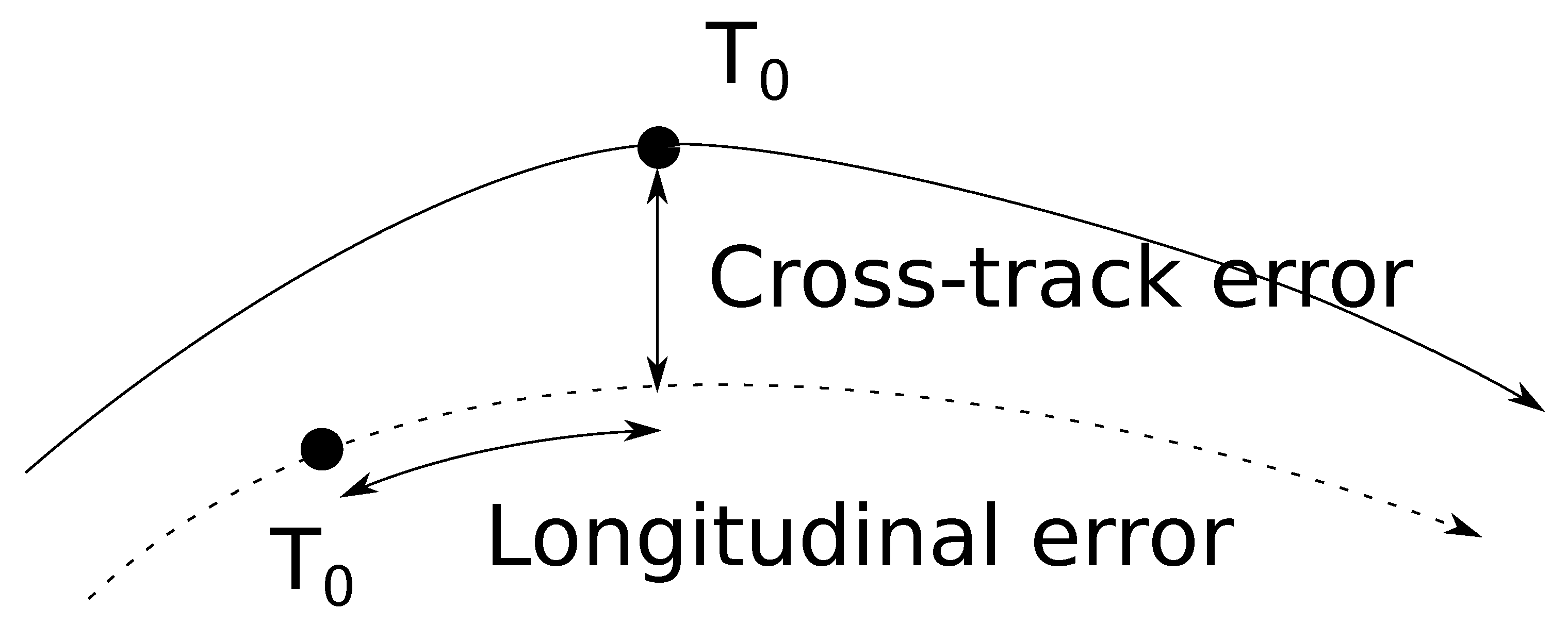
One of the most important sources of uncertainties in the ATM system comes from the wind. When flying a given path, an aircraft can experience two kinds of errors: a cross-track error that describes the lateral deviation from the intended trajectory and a longitudinal error that describes the distance between the current and the expected position at a given time. Figure 1 summarizes these two measures.

FMS are able to deal efficiently with the cross-track error that can be reduced to very low values so that they are generally not a concern, at least during en-route flight phase. Managing the longitudinal error relies on changing the aircraft velocity, mainly by engine thrust adjustment. Such an operation impairs fuel consumption and may not even be possible since during the cruise phase aircraft are operated close to the maximal altitude, significantly reducing the safe interval of speed variation.

As a consequence, keeping an aircraft on a 4D trajectory, that is bound to a given position at a given time, is not realistic, even in the context of future ATM systems like SESAR (Single European Sky ATM Research) or Nextgen. In a real operational context, the flight will fly a sample path of an underlying stochastic process, that is obtained from the reference trajectory by applying a random time change.

To gain a wide social acceptance of the concept, all automated systems must be proven safe, even under uncertainties on aircraft positions and thus must take the above effect into account.

Several automated trajectory planners exist [1], most of them being adapted from their counterparts in robotics, but are generally very sensitive to random perturbations. Navigation functions are of current use for autonomous robots and have been extended to air traffic problems [2]. They offer built-in collision avoidance and are fast to compute. Furthermore, relying basically on a gradient path following algorithm, it is quite easy to derive convergence properties. An interesting approach to design navigation functions is the use of harmonic potentials and recently bi-harmonic ones. The computation is reduced to an elliptic partial differential equation solving, that can be done readily using off-the-shelf software. The STARGATE project, funded by the French agency ANR (Agence Nationale de la Recherche), was initiated to extend harmonic and bi-harmonic navigation functions to a stochastic setting. Within this frame, a mean of simulating random events is required, in order to quantify the probability of failure. As mentioned above, only the longitudinal error along the track is a concern, and it comes from two main sources:

• The airport departure delay and the ATC actions;
• The effect of the wind experienced along the flight path.

Airport or ATC delays may be somewhat anticipated, but an important variability still exists. Concerning the wind, meteorological models are not accurate enough to ensure a good predictability: the best possible description of a wind field is as the sum of a mean component, generally taken to be the output of the atmosphere models, and a random perturbation. Conflict detection under stochastic wind assumption has been addressed for example in [3], where a Monte-Carlo approach was taken to estimate conflict probabilities. The importance of random events in simulation for assessing the robustness of conflict resolution algorithms is pointed out in [4].

Section 3 of this article will be devoted to the means of generating random wind fields, that will be processed within a fast time air traffic simulator. The resulting synthetic flight paths can be used to assess the performance of the conflict solving algorithms and to test the resilience of the planning schemes produced.

In Section 4, a statistical analysis of airport and ATC delays will be presented, and a simple delay generator will be detailed.

In Section 5, numerical implementation issues will be discussed and finally a conclusion will be drawn, along with perspectives for future work.

2. Fast-Time Simulations

Experiments in ATC are often conducted using simulated traffic, as setting up even a small scale real traffic campaign is difficult and expensive. Furthermore, the safety issue of using flying aircraft for studies is barely compatible with a quick assessment of the performance of new concepts. When dealing with simulation, the degree of realism needed depends heavily on the kind of study conducted: investigating flight performance at the aircraft level requires a simulator based on flight dynamics and aerodynamics and will involve realistic physical models. On the other hand, new concepts in ATC can be studied with global, less accurate models that only mimic the expected behavior of the aircraft. In this last case, the execution time and the ability to simulate a large number of flights is more important than the knowledge of the individual states of aircraft. Simulators complying with these needs are called fast-time simulators, in reference to the ability to release trajectories orders of magnitude faster than the actual flight time.

Within the class of fast time simulators, six degrees of freedom (6DOF) ones have the highest accuracy and are closest to the true physics of the aircraft. At the other end of the scale, tabular simulators use precomputed, tabulated performance data that describe an average behavior for a given flight phase: climb, descent, approach, cruise. In the middle, point-mass simulators based on total energy models offer a good compromise between accuracy and ease of implementation. A standard fast-time off the shelf simulator is AirTOp [5], that offers an integrated environment including airports and rule based conflict resolution. For the purpose of the study however, a full control on the simulator code was needed so that this option was not feasible.

The open source fast-time simulator CATS [6] is a lightweight tabular simulator using BADA tables [7] written in CAML (Categorical abstract machine language). It was developed with research applications in mind and is easily configurable. However, since the core software of the STARGATE project was written in Java, interfacing with it is a little bit tricky. Furthermore, it is now quite an old tool, not actively maintained.

A recent (2015) BADA based simulation tool, is Bluesky [8] from TU Delft. It is fully open source and active. It allows for taking a wind field into account, but not with a stochastic component. Being written in Python, it is not easily interfaced with the core part of STARGATE.

Due to the limitations of the aforementioned tools, the development of a complete simulation environment was planned within the frame of the STARGATE project. It was coded almost entirely in pure Java, with only a small portion written in C++ for performance issues. The simulator was nicknamed $\pi$-rats, and includes a very accurate physical model for the taxi part of the flight. The two stochastic components presented below are used respectively to model the uncertainties during the flight and the random take-off delay.

3. Random Wind Field Simulation

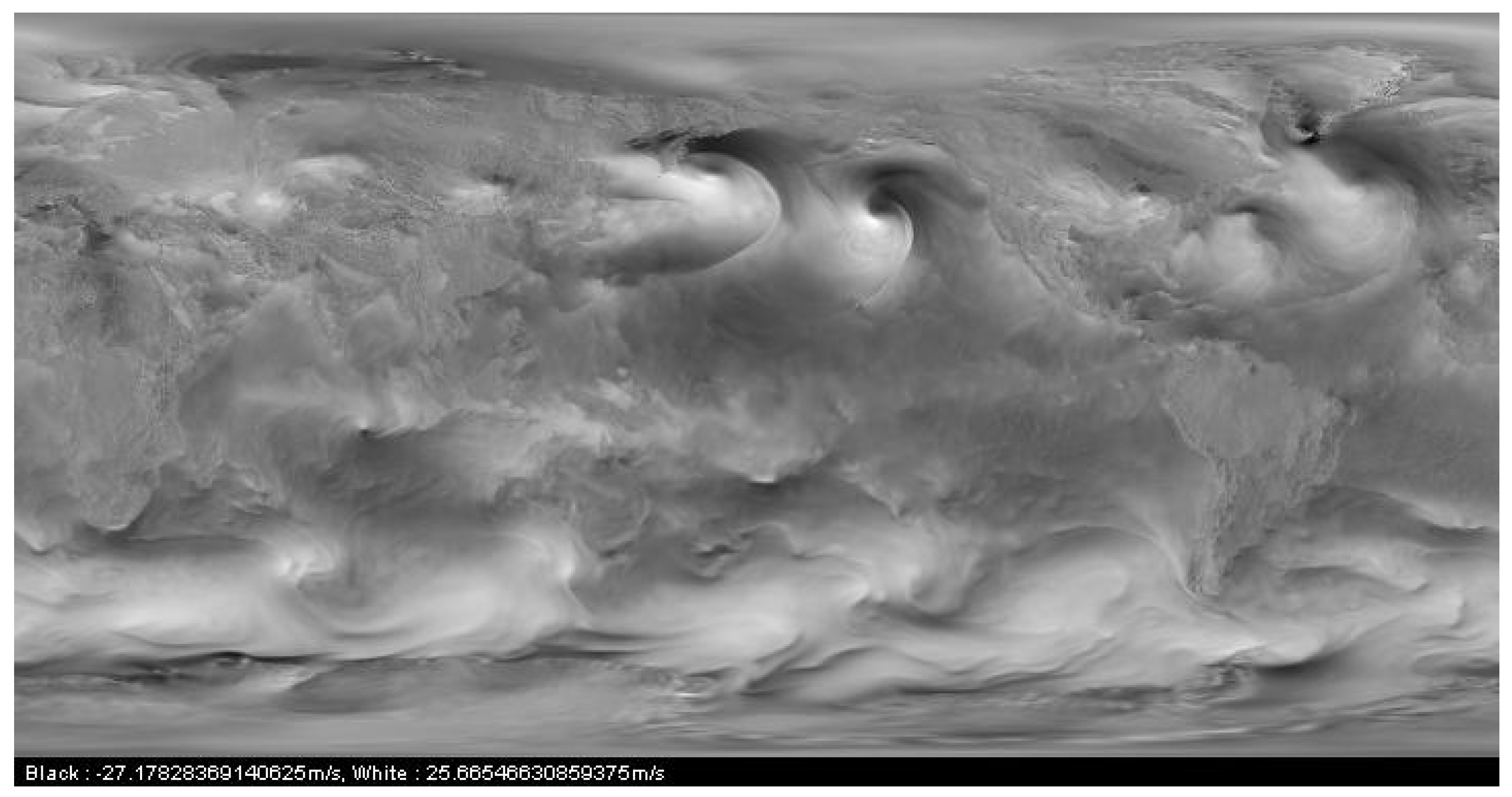
Wind fields generally exhibit an organized structure, along with more chaotic behavior in some areas, as shown in Figure 2.

Meteorological models forecast wind speed on a sampling grid, with angular increments that can be as low as 0.01 degrees (e.g., the AROME model from the French weather service). The temporal resolution is not so high, typically in the hour range. Due to the requirements of future ATM systems, providers are working on an order of magnitude improvement, but such data is not yet available.

Even with the best available resolution, the characteristic mesh size is about 1 km, which is not enough to ensure a very high quality trajectory prediction: an interpolation error will add to the predicted position. The same is true for the time interpolation point of view and both effects may be modeled as a random variable. Finally, inherent model inaccuracies can be incorporated, so that the wind field X may be represented as the sum of a deterministic mean value $X_0$ and a stochastic field $\eta$. While $\eta$ is a vector valued field, it will be described in coordinates and only scalar fields will be considered in the sequel.

3.1. Spectral Representation

In order to be able to simulate a random wind field, a mathematical model of it must be found. This kind of problem pertains to the field of geostatistics [9] and has been investigated in many contexts ranging from mining to economics and weather science. From an intuitive point of view, one wants to construct a random function that maps a position to a vector.

At the most abstract level, a random field is thus a measurable mapping $\eta :U\times \Omega \to {\mathbb{R}}^d$ where $U\subset {\mathbb{R}}^d$ is the domain of definition and $\Omega$ is a probability space that describes the possible outcomes [10]. For a given point x in U, the random variable $\omega \mapsto \eta (x,\omega )$ is the (stochastic) value of the field at position x. It describes the variations of the velocity at x and will be denoted by $\eta \left(x\right)$ in the sequel. According to a theorem of Kolmogorov [10], the knowledge of the probability space $\Omega$ is not required. In fact, a random field is fully characterized by the distribution of its finite samples $(\eta \left(x_1\right),\dots ,\eta \left(x_N\right))$ for any possible choice of the sampling points. When these distributions are normal, the field is said to be Gaussian. It is a very common assumption in geostatistics, backed by the central limit theorem when the randomness of the data comes from a physical noise.

Taking the expectation of $\eta$ and letting x vary over U defines the so-called mean function of the field.

Definition 1.

Let η be a Gaussian field on a domain U of ${\mathbb{R}}^d$. Its mean function is the mapping $\mu :U\to {\mathbb{R}}^d$ defined as:

$$\mu \left(x\right)=E\left[\eta \right(x\left)\right],x\in U$$

The covariance function of the field describes the correlation between velocities:

Definition 2.

Let η be a Gaussian field on a domain U of ${\mathbb{R}}^d$. Its covariance function is the mapping $\tilde{C}:U\times U\to M_d$ defined as:

$$\tilde{C}(x,y)=E\left[(\eta \left(x\right)-\mu \left(x\right)){(\eta \left(y\right)-\mu \left(y\right))}^t\right],(x,y)\in U\times U$$

with $M^d$ the set of square positive definite matrices of dimension d.

The mean and covariance functions fully characterize the Gaussian field $\eta$ [11]. In many cases, the covariance function is translation invariant, meaning that it depends only on the difference between the two measure points and not on their absolute positions. This property is known as spatial stationarity and is expressed as follows:

Definition 3.

Let η be a Gaussian field. It is said to be second order stationary if it exists a mapping $C:U\to M_d$ such that:

$$\forall (x,y)\in U\times U,\tilde{C}(x,y)=C(x-y)$$

The next proposition is classical and can be found in [12] in a more general form.

Proposition 1.

For any finite sequence $(x_1,\dots ,x_n)$ of points in ${\mathbb{R}}^d$, the vector $(X\left(x_1\right),\dots X\left(x_n\right))$ is Gaussian, with mean

$$(\mu \left(x_1\right),\dots ,\mu \left(x_n\right))$$

and covariance

$$\Sigma ={\left(C(x_i-x_j)\right)}_{i,j=1\dots n}$$

The covariance function is positive definite [11] and satisfies:

$$\forall (a_1,\dots a_n)\in \mathbb{R},\forall (x_1,\dots x_n)\in {\Omega }^n,\sum _{i,j}{a}_i{a}_{j}C(x_i-x_j)\ge 0$$

(1)

The Bochner theorem [13] gives a characterization of positive definite functions:

Theorem 1.

A continuous mapping $f:{\mathbb{R}}^d\to \mathbb{R}$ is positive definite if and only if it exists a finite positive measure F such that:

$$\forall x\in \mathbb{R},f\left(x\right)={\int }_{\mathbb{R}}{e}^{i2\pi \langle t,x\rangle }dF\left(t\right)$$

It is often easier to check that a given mapping is positive definite through the use of Theorem 1 than with a direct proof. In the case of covariance functions, F is known as the spectral measure of the random field and when it admits a density $\theta$, one can compute a numerical approximation of it using a discrete Fourier transform. This property is the key ingredient of many efficient random field generators. The spectral density $\theta$ can be proved to be even and positive.

3.2. Gaussian Field Generation

Algorithms for scalar Gaussian field generation can be direct or spectral. In the first case, the Proposition 1 is invoked to generate Gaussian vectors on a mesh of points $(x_1,\dots ,x_N)$ that is generally structured as a rectangular, evenly spaced grid.

Proposition 2.

Let $u=(u_1,\dots ,u_N)$ be a sample of independent, normally distributed real numbers. Let v be a vector in ${\mathbb{R}}^N$ and C a symmetric, positive definite matrix. The vector $C^{1/2}u+v$ is Gaussian, with mean v and covariance C.

Proof. 

It is a very classical result that comes at once from the properties of mathematical expectation. Since u has zero mean:

$$E[C^{1/2}u+v]=C^{1/2}E\left[u\right]+v=v$$

The covariance is then given by:

$$E\left[C^{1/2}u{t}^t{C}^{1/2}\right]=C^{1/2}E\left[u{u}^t\right]C^{1/2}=C^{1/2}{C}^{1/2}=C$$

☐

The computation of the square root $C^{1/2}$ is not required: the Cholesky decomposition $C=L^{t}L$ will give the same result and is much easier to obtain. The algorithmic complexity of the process is dominated by the Cholesky decomposition, that is an $O\left(N^3\right)$ process. Once done, sampling the vector u and performing the combination $Lu+v$ is of order $O\left(N^2\right)$. In many cases, the covariance will quickly drop for distant pairs of points: the matrix C is often nearly sparse, and adapted algorithms for the Cholesky decomposition exist. However, this stage remains the bottleneck of the Gaussian field generation procedure.

Spectral algorithms rely on a fast Fourier transform to let computations occur in the frequency domain. In [14], some methods for sampling Gaussian fields based on this approach are detailed.

The general principle underlying these methods is the use of Bochner theorem and Itô isometry formula. While almost never stated in references related to numerical Gaussian field simulations, it is a very important point that may be used as a basis to derive algorithms. The approach taken in this work is to directly approximate the spectral representation of the field instead of using it only as a convenient tool for lowering the computational cost. A benefit is that optimal quadrature rules may be used in the Fourier domain to improve the reconstruction of the simulated field.

Let us first start with some basic facts about spectral representation of processes as exposed in the reference work [15].

Definition 4.

Let $\mathcal{P}=(\Omega ,\mathcal{T},P)$ be a probability space and let $L^2=L^2(\omega \mathcal{T},P)$ be the space of finite variance complex random variables over it. An orthogonal stochastic measure on $\mathcal{P}$ is a mapping μ from $\mathcal{T}$ to $L^2$ such that:

• $\mu (\varnothing )=0$
• For all couples $(A,B)$ in $\mathcal{T}$ such that $A\cap B=\varnothing$:

  $$\mu (A\cup B)=\mu \left(A\right)+\mu \left(B\right)$$
  P-almost surely.
• It exists a measure m on $\mathcal{T}$ such that for all couples $(A,B)$ in $\mathcal{T}$:

  $$E\left[\mu \left(A\right)\overline{\mu \left(B\right)}\right]=m(A\cap B)$$

The measure m occurring in the Definition 4 is called the structural measure of $\mu$ The definition can be extended straightforwardly to vector valued, finite variance random variables by requiring that the covariance matrix $E\left[\mu \left(A\right)\overline{\mu \left(B\right)}\right]$ is a $\sigma$-additive function on $\mathcal{T}$ with diagonal entries ordinary measures.

Given a simple function $f={\sum }_{i=1}^n{a}_i{1}_{A_i}$, one can define its $\mu$-integral as:

$$\int f\left(x\right)d\mu \left(x\right)=\sum _{i=1}^n{a}_i\mu \left(A_i\right)$$

which is an $L^2$ random variable by definition of $\mu$. Given the fact that random variables in $L^2$ are limits of such functions, one can define the $\mu$-integral of an arbitrary $L^2$ random variable.

A very important isometry theorem holds for $\mu$-integrals.

Theorem 2.

Let $f,g$ be $L^2$ random variables. Then:

$$E\left[\int f\left(x\right)d\mu \left(x\right)\overline{\int g\left(x\right)d\mu \left(x\right)}\right]=\int f\left(x\right)\overline{g}\left(x\right)dm\left(x\right)$$

An important special case arises when $\mu$ is obtained from a left mean-square continuous process F with orthogonal increments. In such a case, one can construct $\mu$ on intervals $[a,b[$ by $\mu \left(\right[a,b\left[\right)=F\left(b\right)-F\left(a\right)$ and extend to the Borel $\sigma$-algebra on $\mathbb{R}$. The resulting $\mu$-integral is a stochastic Stieltjes integral. Extension to ${\mathbb{R}}^d$ can be done component-wise, using independent processes in each coordinate and take as the stochastic measure of a rectangle the product of the stochastic measures of its sides. Itô integral is recovered when F is the Wiener process, the Theorem 2 being the Itô isometry.

Theorem 3.

Let X be a complex stochastic process on $(\Omega ,\mathcal{T},P)$ with a well defined covariance function $C_X$. If it exists a measure space $(A,\mathcal{A},m)$ and measurable functions $g:\Omega \times A\to \mathbb{C}$ such that:

$$\forall ({\omega }_1,{\omega }_2)\in {\Omega }^2,C_X({\omega }_1,{\omega }_2)=\int g({\omega }_1,x)\overline{g({\omega }_2,x)}dm\left(x\right)$$

Then it exists a stochastic orthogonal measure μ on $\mathcal{T}$ with structure measure m such that:

$$X(\omega )=\int g(\omega ,x)d\mu (x)a.e.on\Omega$$

The previous two theorems can be extended to vector-value stochastic processes [15].

The following special case will be the one used in the sequel:

Theorem 4.

Let X be a complex vector valued continuous, stationary random process defined on $\mathbb{R}$ with zero mean. Then it exists a vector-valued stochastic orthogonal measure μ such that almost surely:

$$X\left(t\right)=\int e^{it\xi }d\mu \left(\xi \right)$$

3.3. Principles of Gaussian Fields Simulation

If $\tilde{C}$ is the covariance function of the field that must be simulated, then it can be written according to Theorem 1 as:

$$\forall x,y\in R^d,\tilde{C}(x,y)={\int }_{{\mathbb{R}}^d}exp\left(i\langle x-y,\xi \rangle \right)dF\left(\xi \right)$$

and if $\mu$ is absolutely continuous with respect to the Lebesgue measure as:

$$\forall x,y\in R^d,\tilde{C}(x,y)={\int }_{{\mathbb{R}}^d}exp\left(i2\pi \langle x-y,\xi \rangle \right)\theta \left(\xi \right)d\xi$$

(2)

with $\theta$ a density. Let Z be the centered random field given by:

$$Z_x={\int }_{{\mathbb{R}}^d}exp\left(i2\pi \langle x,\xi \rangle \right){\theta }^{1/2}\left(\xi \right)d{B}_{\xi }$$

(3)

with $B_{\xi }$ the d-dimensional complex Wiener process. By the Itô isometry it comes;

$$\begin{array}{cc}\hfill E\left[Z_x{Z}_y\right]& ={\int }_{{\mathbb{R}}^d}exp\left(i\langle x,\xi \rangle \right)exp\left(i\langle y,\xi \rangle \right)\theta \left(\xi \right)d\xi \hfill \end{array}$$

(4)

$$\begin{array}{cc}& ={\int }_{{\mathbb{R}}^d}exp\left(i2\pi \langle x-y,\xi \rangle \right)\theta \left(\xi \right)d\xi =\tilde{C}(x,y)\hfill \end{array}$$

(5)

Finally, the process $Z_x+\mu \left(x\right)$ has covariance $\tilde{C}$ and mean $\mu$ as required.

For numerical simulations, the above stochastic processes need to generate samples at fixed positions, which may be done using a very simple approximation of the integral as a finite sum. First of all, the domain of integration has to be reduced to a bounded region U of ${\mathbb{R}}^d$ in order to make it amenable to numerical implementation. Since in the spectral representation the density $\theta$ is even, it makes sense to let U be a product of centered rectangles: $U={\prod }_{i=1}^d[-a_i,a_i]$ (here $d=2$ or $d=3$). An elementary cell in the grid, ${\mathcal{C}}_k$, indexed by the vector $k=(k_1,\dots ,k_d)$ with integer coordinates, will be written accordingly as:

$${\mathcal{C}}_k=\prod _{i=1}^d[{\xi }_k^i,{\xi }_{k+1}^i]$$

where for each i, $-a_i={\xi }_0^i<{\xi }_1^i<\cdots <{\xi }_{N_i}^i=a_i$ is a subdivision of the interval $[-a_i,a_i]$. Please note that the index coordinates $k_1,\dots ,k_d$ are for each i in the set $0,\dots ,N_i-1$. The discretization of the integral in (3) over the partition given by the cells ${\mathcal{C}}_k$ using the rectangle quadrature formula gives:

$$Z_x=\sum _{k_1=0,\dots ,k_d=0}^{N_0-1,\dots ,N_d-1}exp\left(i2\pi \langle x,{\xi }_{k_1,\dots ,k_d}\rangle \right){\theta }^{1/2}\left({\xi }_{k_1,\dots ,k_d}\right)V_{k_1,\dots ,k_d}$$

(6)

with:

$$V_{k_1,\dots ,k_d}=\prod _{i=1}^d\left(W_i\left({\xi }_{k_{i+1}}^i\right)-W_i\left({\xi }_{k_i}^i\right)\right)$$

(7)

In the computation of the volume element (7), $W_1,\dots ,W_d$ are independent one-dimensional Wiener processes. Due to the fact that $W_i$ has normally distributed increments, it appears that $V_{k_1,\dots ,k_d}$ follows a d-dimensional centered Gaussian distribution with diagonal covariance matrix and variance ${\xi }_{k_{i+1}}^i-{\xi }_{k_i}^i$ in dimension i: generating samples according to such a law is easily done using for example the Box-Muller algorithm [16].

In practice, only regular grids are used, and we may further assume that discretization steps are equal to a fixed value $\delta$ in each direction. The random number generator is then calibrated once for all to draw samples according to a $\mathcal{N}(0,\delta )$. Please note that the algorithm takes place in the Fourier domain, so characteristic dimensions must be inverted when going to the space domain, as it will be made more precise in the sequel, when dealing with numerical implementation.

3.4. Finding a Covariance Function

Model covariance functions must comply with the requirements already mentioned above, namely they must be a symmetric and of positive type function. Finding a good covariance function is quite a common question arising within the frame of spatial statistics. A good account on the subject is [17] that covers many aspects of covariance functions estimates. As usual with estimators, available methods fall within two categories. In the first one, covariance candidates are selected from a fixed family, whose parameters are adjusted so as to best fit the observations. A classical choice is exponential functions, either in spatial or the Fourier domain: in such a case the transformed function in the dual domain will be a slowly decreasing mapping, behaving roughly as ${\parallel •\parallel }^{-2}$ at infinity. Another option is to use a Gaussian function, that is of positive type and exhibits fast decrease in both the spatial and Fourier domain. Parameters are estimated using a maximum likelihood procedure. Finally, the Matern function [18] is a popular class within the geostatistics community and is defined as:

$$M(x;\nu ,a)=\frac{2^{1-\nu }}{\mathsf{\Gamma }\left(\nu \right)}{\left(a\parallel x\parallel \right)}^{\nu }{K}_{\nu }\left(a\parallel x\parallel \right)$$

(8)

where $K_{\nu }$ is the modified Bessel function of order $\nu$. a is a scale parameter that tunes the model characteristic distance while $\nu$ tunes the smoothness. Large $\nu$ yield very smooth fields while low $\nu$ produce rough ones. While being more accurate for wind field or temperature field simulations, the Matern covariance has the drawback of not having an easily computable Fourier transform. When using the spectral approach for simulations, it must be first evaluated on the same grid as the field to be simulated, then a FFT must be performed in order to have its approximate Fourier transform. Please note that this has to be done only once, regardless of the number of random fields that will be simulated. It has been implemented in the simulator, along with the exponential and Gaussian covariance functions.

The second class of covariance functions, known as non-parametric estimates, is mentioned here for the sake of completeness as it was not implemented for the study. The idea is to build the covariance from the observations themselves, without any assumption about an underlying model. The most commonly used estimators are:

$$\tilde{C}(x,y)={\lambda }^{-1}\sum _{i=1}^n\sum _{j=1}^{n}K\left(\parallel x-x_i\parallel \right)K\left(\parallel y-y_j\parallel \right)X_i{X}_j$$

(9)

where $X_i$ is the observed field at position $x_i$ and:

$$\lambda =\sum _{i=1}^n\sum _{j=1}^{n}K\left(\parallel x-x_i\parallel \right)K\left(\parallel y-y_j\parallel \right)$$

(10)

K is a kernel function that is compactly supported most of the time: as a consequence, the summation takes place on a reduced set of the observation, making the method nearly constant in time if the samples are not too concentrated. As before, computing the Fourier transform requires sampling the covariance function C on a grid. Its main drawback is the number of samples required to get a good estimate and the need to adjust the scale of the kernel in order to get the best possible results.

4. Airport and ATC Delays: A Statistical Study

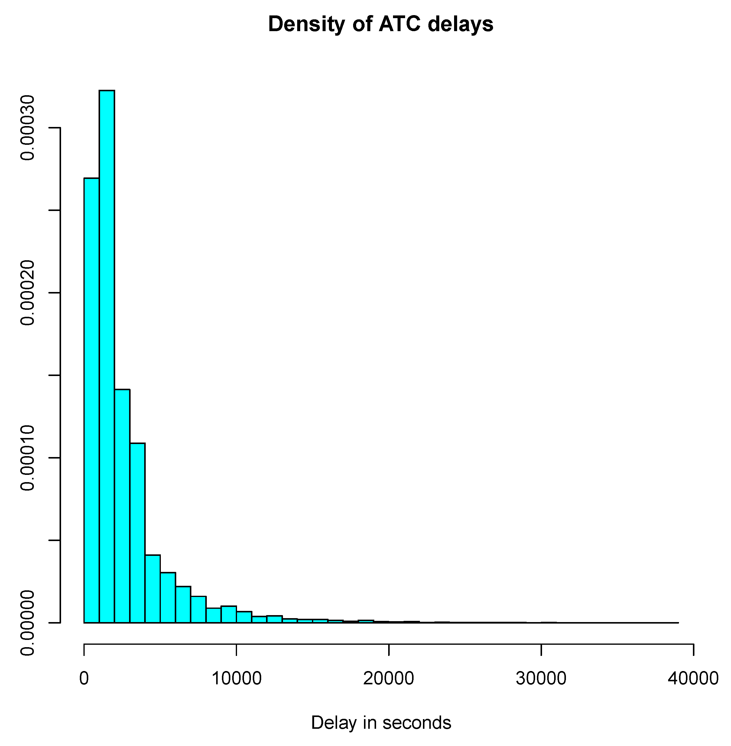
For the purpose of the STARGATE project, only a coarse modeling is needed for the airport delays, as simulations involving ground side are done at a strategical time horizon, namely weeks to days from real departure dates. Given the uncertainties in the weather at this time scale, only very conservative planning may be designed, which will serve as a basis for reference business trajectories negotiation. A statistical study was conducted on sample data coming from flight plans data in France over the years 2012–2015. A python parser was designed in order to transform the original data in COURAGE format (used by the French civil aviation authorities) into a csv file readable in R. The code is made available at the project website [19]. A simple pre-processing step is needed to get rid of aberrant values due to flights erroneously classified on a day, while departing one day before or after. This situation occurs on long-haul flights when part of the trajectory is made over the French airspace, but departure or arrival take place on another day. All flights with high delays are thus processed in order to check for such an event and are discarded from the initial set of samples. Furthermore, negative delays may occur but are uncommon and not useful for the application in mind: only flights with positive ones have been retained in the final sample. The density histogram on the cleaned data is shown on Figure 3.

From classical queuing theory, it is common to fit an exponential distribution on delays. Based on the histogram, other candidates are the Weibull and gamma distributions. Using the function fitdistr from the R package MASS (Modern Applied Statistics with S). the maximum likelihood estimates in

Table 1. Maximum likelihood parameters estimates.

Distribution	Parameters
Exponential	rate = $3.85\times {10}^{-4}$
Gamma	shape = 1.47, rate = $5.66\times {10}^{-4}$
Weibull	shape = 1.13, scale = 2730

were found.

The resulting densities are plotted against the sample histogram in Figure 4.

Only the initial part of the curve makes a real difference, especially for the exponential distribution that will not vanish at the origin. The best fitted distribution is the gamma one, and in fact the exponential distribution is a special case, with the shape parameter equal to 1. For simulation purposes, the generation of exponentially distributed values is easy using either a transformation or the fast ziggurat algorithm [20], making it a first choice from the computational point of view. The exponential distribution yields easier theoretical derivations. It is not a real issue for simulations, but the stochastic delay model is intended to be used also for resilient automatic conflict resolution algorithms. In this context, the ability to derive provable results is mandatory.

The well known absence of memory of the exponential law is questionable in the context of airport or ATC delays as one can expect them to be highly correlated in time. This is true at small time scales, say hours, but no longer verified at the larger time horizons. Depending on the accuracy needed for the model, it may not be an issue. On the other hand, the general gamma distribution is a better choice from the modeling accuracy point of view. The flexibility given by the shape parameter allows a decrease in the likelihood of observing zero delays, which is close to the operational reality. In fact, it is a common practice to allow several aircraft to take-off at the same time. In this case, only one of them will experience zero delay, while the others will be slightly delayed.

Simulating a gamma distribution can be done in a very efficient manner using the reject algorithm presented in [21] since the estimated shape parameter is larger than 1. Let us recall briefly the principle of the rejection method for random variable generation [22]. Let $p_0$ be the target distribution and let ${\pi }_0$ be a reference distribution. Let $p\propto p_0$ and $\pi \propto {\pi }_0$ be two positive functions satisfying $\pi \ge p$. Putting $\theta \left(x\right)=p\left(x\right)/\pi \left(x\right)=\lambda p_0\left(x\right)/{\pi }_0\left(x\right)$ the rejection procedure is given in Algorithm 1.

Algorithm 1 Rejection sampling.

while not accepted do   y is sampled from $p_0$   u is sampled from $U(0,1)$   if $u<\theta \left(y\right)$ then    Accept   end if  end while

The computational efficiency of the algorithm may be low if $\lambda$ is large: finding a reference ${\pi }_0$ as close as possible to $p_0$ is the key ingredient of the method. For shape parameters less than 2, which is the case for the delay samples observed so far, the choice made is to use a reference exponential distribution. Following [23], the optimal rate for this distribution equals the ratio rate/shape of the target gamma distribution, which is $3.85\times {10}^{-4}$ with the above sample of delays. The comparison functions are:

$$\begin{array}{c}\pi \left(x\right)=-25.2exp(-3.85\times {10}^{-4}x),x\ge 0\hfill \\ p\left(x\right)=x^{0.47}exp(-5.66\times {10}^{-4}x),x\ge 0\hfill \end{array}$$

(11)

A simulation was conducted with the generation of ${10}^6$ gamma distributed random variables, yielding an acceptance rate of $0.68$, which is extremely good in such a context. Please note that the computation of the special function $\mathsf{\Gamma }$ is not needed for the rejection method: only exponentials and powers are required.

The overall conclusion for the delays simulation is to use the gamma distribution with the rejection algorithm. It yields close to operational values, with only a small increase in computational cost when compared to the exponential distribution. For theoretical derivations, the exponential distribution is the best suited, but the above result shows that it is a close approximation of the gamma.

Finally, it is worth mentioning that gamma distributions can be represented as points on a two dimensional Riemannian manifold [24]. Using this geometrical framework will pave the way to a very accurate description of the structure of delays, by performing clustering on the gamma manifold. The final result will be an empirical distribution of gamma distributions, allowing for the generation of different delays structure, possibly taking into account spatial informations. This extension is currently under investigation, the main issue being the availability of the delays at the airport level.

5. Numerical Implementation

The purpose of this section is to detail the way random wind fields are generated. It is split into two parts: acquisition of weather data, with an emphasis on publicly accessible sources and stochastic simulation.

5.1. Weather Data

The overall simulation process starts with prior information about the deterministic component of the field. It is available from weather services as a grid of values computed from a numerical model. Depending on the reference time, real measurements may be part of the data, but will not cover the entire grid: an interpolation is realized implicitly by the model used. The French weather agency provides two ways for accessing the data:

• Direct download of files encoded in the GRIB (GRIdded Binary) format [25].
• Access through a web service complying with the European INSPIRE (Infrastructure for spatial information in Europe) directive [26].

The highest resolutions can be obtained only using the first procedure.

Table 2. Weather data downloadable from Meteo France.

Area	Grid Step	Model	Coverage (Lat-Lon)
Europe	0.1 deg	ARPEGE	72${}^{\circ }$ N 20${}^{\circ }$ N 32${}^{\circ }$ W 42${}^{\circ }$ E
Globe	0.5 deg	ARPEGE	World
France	0.01 deg	AROME	55.4${}^{\circ }$ N 37.5${}^{\circ }$ N 12${}^{\circ }$ W 16${}^{\circ }$ E
France	0.025 deg	AROME	53${}^{\circ }$ N 38${}^{\circ }$ N 8${}^{\circ }$ W 12${}^{\circ }$ E

summarizes the data downloadable with the associated grid spacing and coverage, expressed in latitude-longitude coordinates.

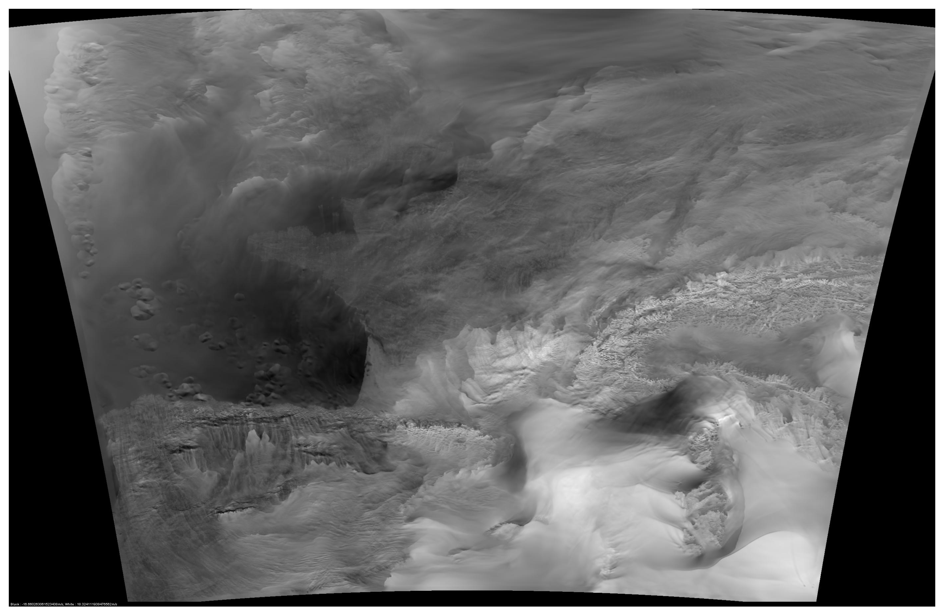
Nearly all atmospheric parameters are available. The complete description of the AROME and ARPEGE models is available at [27]. Figure 5 is an example of wind data acquired from the 0.01 deg AROME model.

Unfortunately, high resolution data cannot be accessed from the web service at the time where this article was written, only the 2.5 deg world coverage was implemented. It is expected that all models will soon be ported to this platform, which will then become the preferred data source. Due to the resolution limitations and the fact that fine step samples are needed to accurately implement the random field generation, only the outputs from the AROME model were used in the present work. The relevant atmospheric parameters were the $u,v$ wind components, associated respectively to projections onto local longitude and latitude coordinates and with an altitude-pressure of 250 hPa, roughly equal to the flight level 340, which is the mean cruise altitude for commercial aircraft (one must note that resolution is reduced at this altitude compared to the original 0.01 deg).

5.2. Gaussian Field Simulation

As indicated in Section 3, the simulation will be conducted by means of a spectral representation. The fast Fourier transform (FFT) is an $O(nlogn)$ algorithm for efficiently computing sums like the one appearing in (6). The software library used for that purpose is FFTW [28,29], a very efficient implementation that is able to operate on sequences of arbitrary lengths (The original FFT algorithms requires lengths in powers of two).

Let us first recall the definition of a discrete Fourier transform (DFT), that is computed by the FFT algorithm. Given a sequence $x_0,\dots ,x_{N-1}$, its DFT is the sequence $\widehat{x_0},\dots ,\widehat{x_{N-1}}$ given by:

$$\widehat{x_k}=\sum _{j=0}^{N-1}{x}_j{e}^{-i2\pi \frac{jk}{N}}$$

(12)

Looking at expression (12), it appears immediately that $\widehat{x_k}$ is a periodic sequence, of period N. Furthermore, if the DFT is interpreted as an approximation of a Fourier integral, then the domain of integration has length 1, due to the $j/N$ appearing in the complex exponential. The inverse DFT is defined pretty much the same way:

$$x_k=\frac{1}{N}\sum _{j=0}^{N-1}{\widehat{x}}_j{e}^{i2\pi \frac{jk}{N}}$$

(13)

The DFT can be used to approximate an integral if considered as a Riemann sum. In such a case, it is easy to see that if the points $x_j,j=0\dots N-1$ are considered as samples at positions $jT/N$ in the interval $[O,T[$, so that the time period is T, then the corresponding sample positions in the frequency domain are located at $k/T,k=0\dots N-1$. Introducing the so-called sampling frequency $f_s=N/T$, the samples in the frequency domain are expressed as $k{f}_s/N,k=0\dots N-1$. Going back to formula (7), the points ${\xi }_j^i$ appearing in the expression correspond to a subdivision of the interval $[-f_s^i/2,f_s^i/2]$ where $f_s^i$ is the sampling frequency in the dimension i (with corresponding number of samples $N_i$). This fact is important and often overlooked: the frequency domain depends on the sampling rate, and thus if the time (or spatial) interval is fixed, on the number of discretization points. On the other hand, the frequency resolution, that is the difference between two samples in the Fourier domain depends only on T, the length of the time interval. As a consequence, the respective variances of the Gaussian increments occurring in the expression (7) are $1/T_i$, where $T_i$ is the length of the spatial domain in dimension i, and are not dependent on the number of sampling points. The same remark applies for the function $\theta$ appearing in (7) where care must be taken to use the points ${\xi }_i=(k-N_i/2)/T_i,k=0\dots N_i$. When using the inverse DFT for computing, it is important to note that the term $1/N$ present in the expression must be scaled out in order to get an approximate integral. Finally, the procedure described above will generate a complex valued random field, which is not needed in practice, unless one wants to obtain two independent samples in one step. It is possible to get a real valued field by generating only half of the Gaussian random variables and taking the complex conjugate of them for the remaining ones. Gathering things, a 2D-field generation algorithm on a evenly spaced grid with $N_x,N_y$ points in each coordinate, can be summarized as indicated below.

Algorithm 2 returns a field with energy proportional to the product $f_x{f}_y$. This can be understood intuitively by recalling that the DFT approximates an integral over $[-f_x/2,f_x/2]\times [-f_y/2,f_y/2]$. If a unit energy is needed, then an inverse scaling must be applied or a normalization performed: this last option is preferred as it removes any inaccuracy coming from the finite precision computation of the FFT, at the expense of a higher computational cost.

Algorithm 2 2D Gaussian field generation.

Require:M is a $N_x\times N_y$ complex matrix Require: $f_x,f_y$ are the respective sample frequencies in $x,y$ Require: $\theta$ is the required spectral density Require: $N(\mu ,\sigma )$ generates independent random normally distributed real numbers with mean $\mu$ and variance $\sigma$  for $i=0\dots N_x-1$ do   for $j=0\dots N_y-1$ do       ▹ Endpoints are handled differently: they have a vanishing imaginary part    if $i==0$ or $j==0$ or $i==N_x/2$ or $j==N_y/2$ then     $\Re M(i,j)\leftarrow N(0,f_x\ast f_y)$     $\Im M(i,j)\leftarrow 0$    else     $\Re M(i,j)\leftarrow N(0,f_x\ast f_y)\ast {\theta }^{1/2}({\xi }_i,{\xi }_j)$     $\Im M(i,j)\leftarrow N(0,f_x\ast f_y)\ast {\theta }^{1/2}({\xi }_i,{\xi }_j)$     $M(N_x-i,N_y-j)=\overline{M(i,j)}$    end if   end for   $X\leftarrow N_x\ast N_y\ast IFFT\left(M\right)$  end for                  ▹ X is the generated real field

5.3. Hardware and Software Architecture

The complete $\pi$-rats framework is a fast-time simulator written in Java and able to perform parallel computations on a grid of computers. Each compute node hosts a simulation process and communicates with a master node using MPICH3 and the Java Native Interface (JNI) API. In the current implementation, nodes are Fujitsu Celsius workstations with gigabyte links, a dual XEON E5-2609 at 2.5 GHz and 16 GB of RAM memory. The master workstation is also used for sandbox development and has a Pascal Titan X GPU card attached. Future releases of the simulation environment, including the random wind field simulator, will make use of GPU computing power when available.

The random delay generator does not significantly impact the overall computation cost since it is used only when a flight is scheduled for departure. It was implanted in pure Java, without any third-party library. Its performance was assessed both on qualitative and quantitative aspects using a database of flight plans filled and realized in the French airspace and covering the 2016–2017 period. According to French Civil Aviation School (ENAC) operational experts, the simulated departure delays are coherent with their experience on French airports.

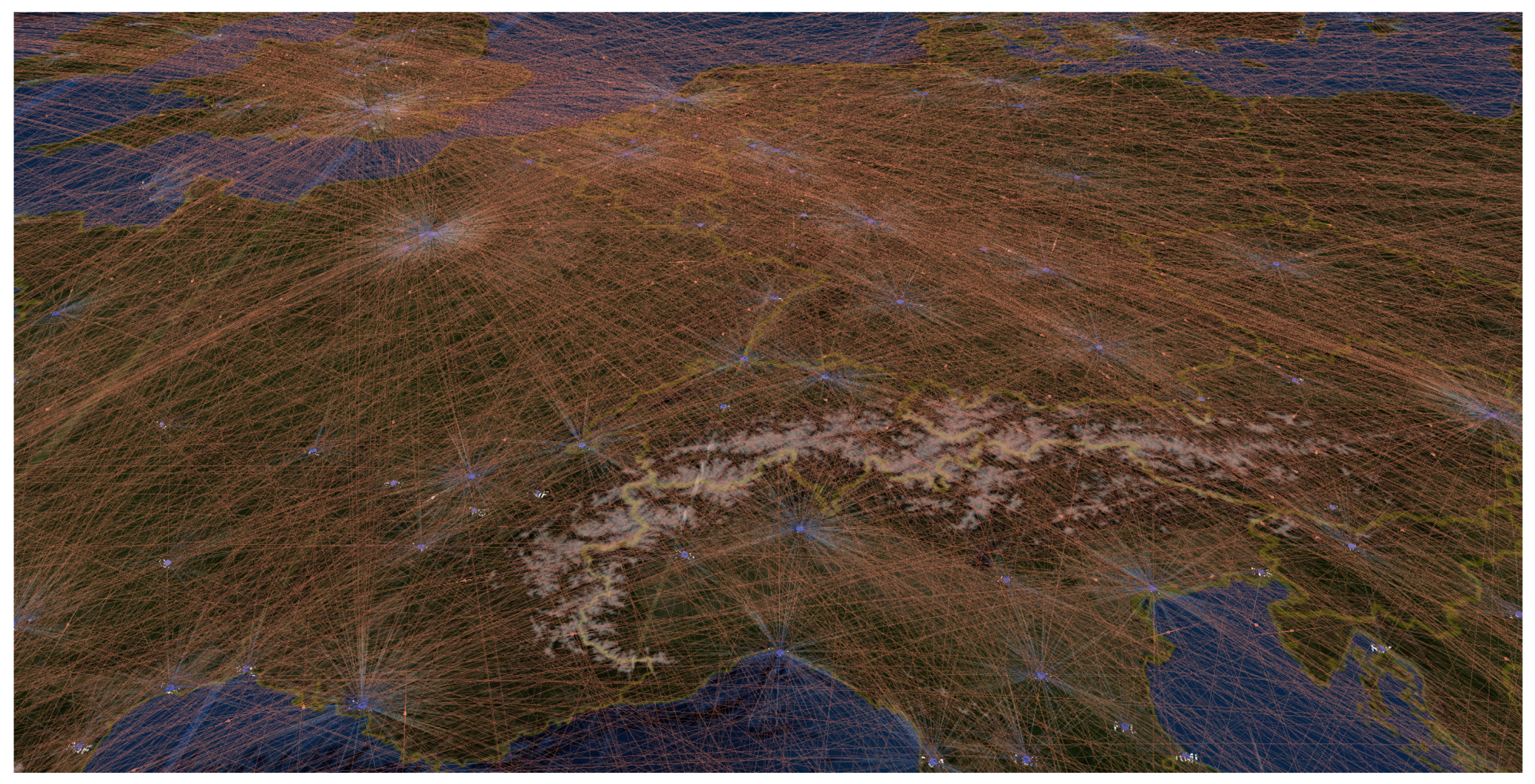
The bottleneck of the wind field simulator is the two dimensional Fourier transform. It is performed using the FFTW v3.3.7 library, which is one of the most efficient software implementations of the FFT algorithm available today. It has the ability to exploit all the cores and processors available on the compute platform. On the master node described above, the simulation of a day of traffic over France (approx. 8000 flights), with refreshing rate of 4 s, takes less than 10 min. One day of world traffic can be simulated on a grid of six nodes in 20 min. A snapshot of simulated traffic is given in Figure 6.

6. Conclusions and Future Work

The present work describes means of simulating random events occurring in the context of the air traffic system. ATC and airports delays can be modeled according to a gamma distribution, taking into account the large time horizon considered. This choice was backed by expert advice, which justifies its use in a research oriented simulator. For the meteorological uncertainties, a simple random Gaussian field model is assumed. Generating such samples can be done efficiently using a spectral algorithm. This approach is based on the spectral representation of the process and its discretization in the Fourier domain, which contrasts with the usual spatial discretization. The resulting algorithm is similar to the ones described in the literature, but relies on a different principle and allows more flexibility. A direct extension can be done to deal with multiscale simulation of wind fields, effectively representing turbulent phenomenons, like those occurring in approach phases. While not implemented in the current release of the simulator, the use of wavelets for representing the covariance functions will be introduced in a future work to cope with multiscale modeling. Finally, it is worth mentioning that a UAV extension of the $\pi$-rats simulator is under development and will be made available on [19] at the beginning of 2019.

References

- Goerzen, C.; Kong, Z.; Mettler, B. A Survey of Motion Planning Algorithms from the Perspective of Autonomous UAV Guidance. J. Intell. Robot. Syst. 2009, 57, 65–100. [Google Scholar] [CrossRef]
- Roussos, G.P.; Kyriakopoulos, K.J. Completely decentralised Navigation Functions for agents with finite sensing regions with application in aircraft conflict resolution. In Proceedings of the 2011 50th IEEE Conference on Decision and Control and European Control Conference (CDC-ECC), Orlando, FL, USA, 12–15 December 2011. [Google Scholar]
- Hu, J.; Prandini, M.; Sastry, S. Aircraft conflict prediction in the presence of a spatially correlated wind field. IEEE Trans. Intell. Transp. Syst. 2005, 6, 326–340. [Google Scholar] [CrossRef]
- Rey, D.; Rapine, C.; Fondacci, R.; Faouzi, N.E.E. Subliminal Speed Control in Air Traffic Management: Optimization and Simulation. Transp. Sci. 2016, 50, 240–262. [Google Scholar] [CrossRef]
- AirTop Simulator. Available online: http://airtopsoft.com/ (accessed on 1 March 2018).
- Alliot, J.M.; Bosc, J.F.; Durand, N.; Maugis, L. CATS: A complete air traffic simulator. In Proceedings of the 16th Digital Avionics Systems Conference (DASC 1997), Irvine, CA, USA, 30 October 1997; Volume 2, pp. 8.2-30–8.2-37. [Google Scholar]
- BADA Aircraft Database. Available online: http://www.eurocontrol.int/services/bada (accessed on 1 March 2018).
- Bluesky Simulator. Available online: http://homepage.tudelft.nl/7p97s/BlueSky/ (accessed on 1 March 2018).
- Chilès, J.; Delfiner, P. Geostatistics: Modeling Spatial Uncertainty; Wiley Series in Probability and Statistics; Wiley: Hoboken, NJ, USA, 1999. [Google Scholar]
- Doob, J. Stochastic Processes; Wiley Publications in Statistics; Wiley: Hoboken, NJ, USA, 1990. [Google Scholar]
- Mandrekar, V.; Gawarecki, L. Stochastic Analysis for Gaussian Random Processes and Fields: With Applications; Chapman & Hall/CRC Monographs on Statistics & Applied Probability; CRC Press: Boca Raton, FL, USA, 2015. [Google Scholar]
- Kotz, S.; Gikhman, I.; Skorokhod, A. The Theory of Stochastic Processes I; Classics in Mathematics; Springer: Berlin/Heidelberg, Germany, 2015. [Google Scholar]
- Rudin, W. Fourier Analysis on Groups; Dover Books on Mathematics; Dover Publications: Mineola, NY, USA, 2017. [Google Scholar]
- Lang, A.; Potthoff, J. Fast simulation of Gaussian random fields. Monte Carlo Meth. Appl. 2011, 17, 195–214. [Google Scholar] [CrossRef]
- Gikhman, I.; Skorokhod, A. Introduction to the Theory of Random Processes; Dover books on Mathematics; Dover Publications: Mineola, NY, USA, 1969. [Google Scholar]
- Box, G.E.P.; Muller, M.E. A Note on the Generation of Random Normal Deviates. Ann. Math. Stat. 1958, 29, 610–611. [Google Scholar] [CrossRef]
- Genton, M.G.; Kleiber, W. Cross-Covariance Functions for Multivariate Geostatistics. Stat. Sci. 2015, 30, 147–163. [Google Scholar] [CrossRef]
- Guttorp, P.; Gneiting, T. Studies in the history of probability and statistics XLIX On the Matérn correlation family. Biometrika 2006, 93, 989–995. [Google Scholar] [CrossRef]
- Open Source Code Repository for the STARGATE Project. Available online: https://stargate.recherche.enac.fr/ (accessed on 1 March 2018).
- Marsaglia, G.; Tsang, W.W. The Ziggurat Method for Generating Random Variables. J. Stat. Softw. 2000, 5, 1–7. [Google Scholar] [CrossRef]
- Martino, L.; Luengo, D.; Míguez, J. Independent Random Sampling Methods; Statistics and Computing; Springer: Cham, Switzerland, 2018. [Google Scholar]
- Dagpunar, J. Principles of Random Variate Generation; Includes Index; Clarendon Press: Oxford, UK, 1988. [Google Scholar]
- Martino, L.; Luengo, D. Extremely efficient generation of Gamma random variables for α ≥ 1. arXiv, 2013; arXiv:stat.CO/1304.3800. [Google Scholar]
- Dodson, C. Information geodesics for gamma models of communication clustering. J. Stat. Comput. Simul. 2000, 65, 133–146. [Google Scholar] [CrossRef]
- Public Data Downloading from Meteo France. Available online: https://donneespubliques.meteofrance.fr/?fond=rubrique&id_rubrique=51 (accessed on 1 March 2018).
- Meteo France Web Service. Available online: https://donneespubliques.meteofrance.fr/?fond=geoservices&id_dossier=14 (accessed on 1 March 2018).
- Arpege and Arome Models Manuals. Available online: https://donneespubliques.meteofrance.fr/client/document/description_parametres_modeles-arpege-arome-v2_185.pdf (accessed on 1 March 2018).
- FFTW Website. Available online: http://www.fftw.org/ (accessed on 1 March 2018).
- Frigo, M.; Johnson, S.G. The Design and Implementation of FFTW3. Proc. IEEE 2005, 93, 216–231. [Google Scholar] [CrossRef]
Figure 1.
Longitudinal and cross-track errors.
Figure 2.
A typical wind field (world coverage).
Figure 3.
Density of delays.
Figure 4.
Maximum likelihood fits.
Figure 5.
Wind v-component (0.01 deg resolution).
Figure 6.
Traffic simulation before business trajectory negotiation.