A Multi-Fidelity Approach for Aerodynamic Performance Computations of Formation Flight

Abstract

This paper introduces a multi-fidelity computational framework for the analysis of aerodynamic performance of flight formation. The Vortex Lattice and Reynolds Averaged Navier–Stokes methods form the basis of the framework, as low- and high-fidelity, respectively. Initially, the computational framework is validated for an isolated wing, and then two rectangular NACA23012 wings are considered for assessing the aerodynamic performance of this formation; the optimal relative position is through the multi-fidelity framework based on the total drag reduction. The performance estimates are in good agreement with experimental measurements of the same configuration. Total aerodynamic performance of formation flight is also assessed with respect to attitude variations of the lifting bodies involved. The framework is also employed to determine the optimal position of blended-wing-body unmanned aerial vehicles in tandem formation flight.

1. Introduction

It is widely known that aeroplanes flying in formation yield fuel savings. Fuel savings are achieved due to the reduced induced drag on the following aeroplane, when it is positioned within the upwash created by the leader’s wingtip vortices. It has been established experimentally and computationally that birds flying in formation results in energy savings [1,2]. Lissaman and Shollenberg [3] showed that at the optimal distance between the leader and the followers in a flock of twenty-five birds could increase the flight range by $70\%$ compared to their isolated flights. Hainsberg [4] used fifty-five geese against the model of Lissaman and Schollenberger which reflected the power savings of $36\%$. Hummel [5] devised a theory to predict the optimal wing tip spacing $(WT{S}_{OPT}=0.5b(1-0.89))$ for the maximum drag reduction and concluded that it is a negative value which is only possible in the V-shaped formation configurations. Use of lifting line theory to study formation and control has also been of keen interest for researchers [6].

Unmanned Aerial Vehicles (UAVs) have been incorporated in civilian and military fields for surveillance, reconnaissance, search and rescue missions and UAV swarms have been proved to be more performance efficient in formations [7,8].

Many in-flight tests, wind tunnel experiments and computational analyses were performed in recent decades to study formation flight. Hummel and Beukenberg [5] conducted an experiment using two Dornier Do-28 aircraft and established that the maximum obtainable power savings are of about $15\%$. Pahle and Berger [9] tested several flights for large transport class vehicle C-17 aircraft with maximum fuel savings of 7–8%. Inasawa et al. [10] used two rectangular wings of aspect ratio (AR) 5 in a wind tunnel while Blake and Gingras [11] tested two delta wings and compared against the analysis obtained from Vortex Lattice Method (VLM). Recently, Slotnick et al. [12] performed aerodynamic analysis using a multi-fidelity approach. The analysis performed used low-fidelity VLM along with high-fidelity hybrid RANS solver and established the total drag benefits of around $25\%$, which was validated against flight test data with good agreement.

Formation flights involving more than just one follower have also been the prime focus of research to quantify individual savings and the resulting overall drag reduction of the aerodynamic system [13]. Blake and Multhopp [14] showed that $10\%$ wing span overlap between the leader and the follower could result in $60\%$ increase in the flight range for a cluster of five aircraft in V formation while Maskew et al. [15] found the flight range augmentation of 46–67% for three to five aircraft. It was further noted that power savings were more in the case of second follower than the first. Wagner et al. [16] confirmed increased savings of $17.5\%$ for the second wingman compared to first which yielded $15\%$ savings [17]. Recently, Ivan and Roberts [18] conducted wing tunnel tests using multiple wings configurations with each wing having low aspect ratio of two; a total power savings of $14\%$ and $24\%$ in two and three wings configurations was obtained. In correspondence to finding an optimum spacing between the various units in formation, numerous studies also shed light on effect of leader’s shape and size on the follower [19,20].

The present study involves the development of flexible and robust multi-fidelity numerical framework for studying formation flight. The numerical framework accuracy is assessed with grid/panel sensitivity analysis and comparison with experimental data. A computational analysis of two identical NACA 23012 rectangular wings in formation using the multi-fidelity approach of RANS and VLM methodologies is compared against Inasawa et al. [10] experimental data. Furthermore, to demonstrate the flexibility of the numerical framework, two blended-wing aircraft in formation flight are modelled. Section 2 introduces the governing equations for VLM and RANS along with mesh generation strategy and solver attributes. Section 3 expands on the aerodynamic performance analysis of an isolated NACA23012 wing and also in two wings of the same configuration in tandem formation, the local angle of incident and the relative position is in order to maximise performance gains. The computational analysis is further augmented by altering the angle of attack of the lead wing and its effect on the trail wing is assessed. Furthermore, two blended-wing-body aircraft in formation are introduced and the aerodynamic performance is assessed within the multi-fidelity approach. Finally, the conclusions are presented in Section 4 comprising of the inferences obtained for both computational techniques and their applicability to analysis.

2. Computational Methodology

Multi-fidelity strategies incorporating different levels of uncertainty for aerodynamic performance estimations are becoming a standard tool for design, parameterisation and optimisation tasks for aircraft systems. Inexpensive methods based on panels, lifting line theory and vortex lattice methods can generate large data sets for design of experiment phases and multi-objective optimisation analysis. The limitations of these methods with respect to the inherited physical assumptions must be considered, as their applicability range has to be tailored to produce realistic aerodynamic performance indicators particularly in terms of drag estimation. Higher fidelity approaches such as Navier–Stokes solvers can be used to complement the predictions of the lower fidelity approaches.

The computational approach adopted for this study is based on the Vortex Lattice Method solving the Laplace’s equation, where each discrete element corresponds to the vortex line solution of the incompressible potential flow equation. The open-source VLM code Tornado [21] is employed as the foundation of the low-fidelity framework. Additional modules are developed enabling individual trim conditions and Cartesian coordinates to be set for multiple surfaces representing additional lift-generating bodies. High-fidelity aerodynamic estimations are obtained with a second-order RANS solver that accounts for three-dimensionality of the flow, turbulence, viscous drag and boundary layer effects. The developed low-fidelity framework enables the construction of extensive simulation data sets for large flight formation configurations to run in a fraction of the computational cost compared with the RANS approach.

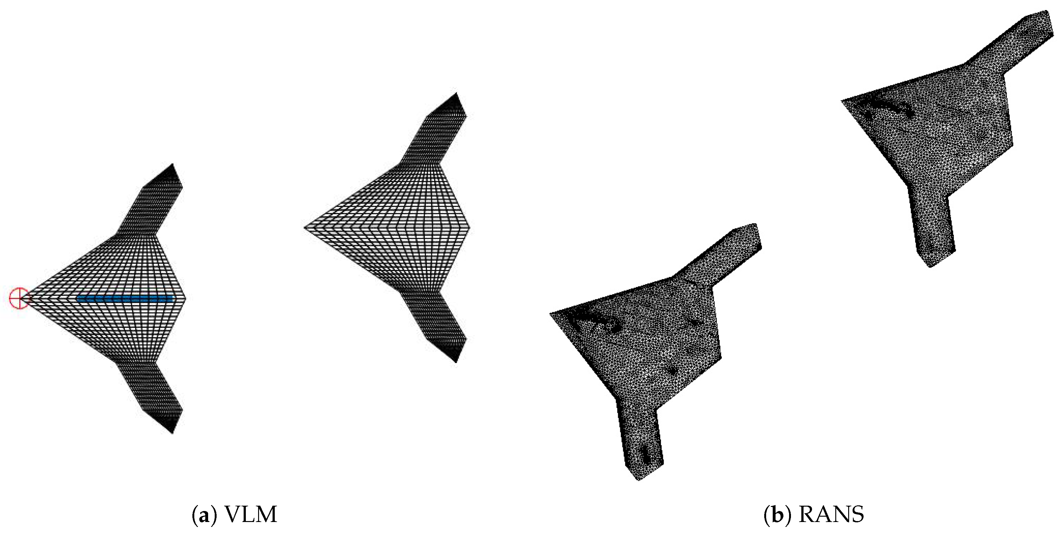
2.1. Low-Fidelity: Vortex Lattice Method

Vortex Lattice Method assumes that the flow is incompressible, inviscid and irrotational. The resulting velocity field is assumed to be a conservative vector field which essentially means that a scalar velocity potential $\varphi$ whose gradient will produce a velocity vector field combined with the free stream velocity as given in Equation (1).

$$\mathit{V}={\mathit{V}}_{\infty }+\nabla \varphi$$

(1)

The velocity field has to satisfy the incompressible continuity equation written as

$$\nabla ·\mathit{V}=0$$

(2)

the assumed conservative vector field is the velocity field expressed in terms of scalar potential ${\varphi }_{}$ that results in it being satisfied, given by

$${\nabla }^2\varphi =0$$

(3)

The scalar potential $\varphi$ satisfies the Laplace’s equation which further implies that if ${\varphi }_1$ and ${\varphi }_2$ are two potential solutions then their linear combination such as $c_1{\varphi }_1$ + $c_2{\varphi }_2$ is also a solution for any values of $c_1$ and $c_2$. This forms the potential flow theory in which such solutions are combined together to represent a lifting surface. VLM uses one such elementary potential solution to form a vortex sheet and represent a lifting surface.

The thickness of the lifting surface is ignored and the planform of a cambered surface is divided into a number of quadrilateral panels as shown in Figure 1. The number of panels to be incorporated for a particular analysis is subjected to the required accuracy. The lifting surface is replaced with a vortex sling on each panel such that the bound vortex part of the sling is placed at 1/4 chord line. Solution of the velocity field at each panel is computed, based on the attributed vortex sheet of the unknown strength ${\Gamma }_j$ on the corresponding panel. A normal vector $\mathit{n}$ at every panel is calculated respective collocation points accounting for camber of the lifting surface. For a problem consisting of N number of panels, the perturbation velocity at ith collocation point is given in Equation (4).

$${\nabla }_{{\varphi }_i}=+{\sum }_{j=i}^N{\mathit{w}}_{ij}{\Gamma }_j$$

(4)

The free-stream velocity components are given in terms of angle of attack ($\alpha$) and angle of side slip ($\beta$), as given in Equation (5), and are depicted in Figure 2a,b.

$${\mathit{V}}_{\infty }=V_{\infty }\left[\begin{array}{c}cos\left(\alpha \right)cos\left(\beta \right)\\ -sin\left(\beta \right)\\ sin\left(\alpha \right)cos\left(\beta \right)\end{array}\right]$$

(5)

Note that for the present study the angle of side slip ($\beta$) is zero. For a problem with N panels, the perturbation velocity at collocation point i is given by summing the contributions of all the horseshoe vortices in terms of an Aerodynamic Influence Coefficient (AIC) matrix ${\mathit{w}}_{ij}$. A physical boundary condition of no normal flow component to each panel of the lifting surface is applied and is expressed by Equation (6) at the collocation points.

$${\mathit{V}}_{\mathit{i}}·{\mathit{n}}_{\mathit{i}}=\left({\mathit{V}}_{\infty }+{\sum }_{j=i}^N{\mathit{w}}_{ij}{\Gamma }_j\right)$$

(6)

This is demonstrated in Figure 2c,d. This is also known as flow tangency condition. After evaluating the dot products, a new normal-wash aerodynamic influence coefficient (AIC) matrix is formed given by $a_{ij}$ = ${\mathit{w}}_{ij}·{\mathit{n}}_{\mathit{i}}$, as given in Equation (7)

$$\left[\begin{array}{cccccc}{a}_{11}& a_{12}& .& .& .& a_{1n}\\ a_{21}& .& .& .& .& .\\ .& .& .& .& .& .\\ .& .& .& .& .& .\\ a_{n1}& a_{n2}& .& .& .& a_{nn}\end{array}\right]\left[\begin{array}{c}{\Gamma }_1\\ {\Gamma }_2\\ .\\ .\\ {\Gamma }_n\end{array}\right]=\left[\begin{array}{c}{b}_1\\ b_2\\ .\\ .\\ b_n\end{array}\right],$$

(7)

the right hand side of the equation is formed by a free-stream velocity and the two aerodynamic angles given below (8).

$${\mathit{b}}_{\mathit{i}}=V_{\infty }\left[\begin{array}{c}cos\left(\alpha \right)cos\left(\beta \right),-sin\left(\beta \right),sin\left(\alpha \right)cos\left(\beta \right)\end{array}\right]·{\mathit{n}}_{\mathit{i}}$$

(8)

A horseshoe vortex is imparted to the panel which starts from several lengths downstream and moves forward to the panel and crosses it at the quarter chord line and then again runs to the far down stream. All the vortices create downwash on each panel on the lifting surface. ${\mathit{V}}_{\mathit{ind}}$ is the induced velocity at the centre of the panel which is calculated once the vortex strength is evaluated using Biot–Savarts Law given by Equation (9).

$$d{\mathit{V}}_{\mathit{ind}}=\frac{\Gamma }{4\pi }\frac{dl\times \mathit{r}}{{\left|r\right|}^3}$$

(9)

The induced flow is used to get the force acting on the panel by using Kutta–Jukovski theorem given by Equation (10)

$${\mathit{F}}_i=\rho {\Gamma }_i(V_{\infty }+V_{ind})\times {\mathit{l}}_i$$

(10)

where ${\mathit{F}}_i$ is the force contribution from the ith panel, $\rho$ is the air density, ${\mathit{l}}_i$ is the vortex transverse segment vector (bound vortex) of that panel and ${\mathit{r}}_i$ is the position vector of the segment’s centre. The wake is assumed to be flat and in the position in the free-stream direction, as shown in Figure 2b.

The VLM code is based on the Tornado solver. Several modules are created that provide the control of the non-dimensionalised lateral ($l/s$), vertical ($h/c$) and longitudinal ($x/c$) coordinates for n number of wings, as shown in Figure 3 for a rectangular wing of the NACA23012 configuration. The modules include the development of the connectivity of multiple wings based upon the number of panels associated with the respective wing. The right hand side term of the boundary condition given in Equation (7) is split. The value of $\alpha$ in the term $-V_{\infty }sin\left(\alpha \right)$ is the angle of attack. Splitting the right hand side of the boundary condition is achieved by assigning a different value of $\alpha$ for the lead and trail wing depending upon the number of panels associated with that wing. The resulting vector can then be obtained using the same procedure discussed within this section; the method first solves for the aerodynamic forces on the nth wing in locally altered coordinates. Their effect on the other members of the formation is analysed by comparing the aerodynamic coefficients attributed for each wing. Simulations are run to find an optimized solution by constructing a matrix for longitudinal and lateral overlapping positions of the wings. The resulting matrix of the aerodynamic coefficients is plotted for all the lateral and longitudinal positions of the trail wing at a particular stream-wise distance and is discussed in detail in Section 3.3. The developed VLM framework also enables flight dynamics of attitude parameters including pitch, yaw and roll angles to be set for each individual aircraft or wing.

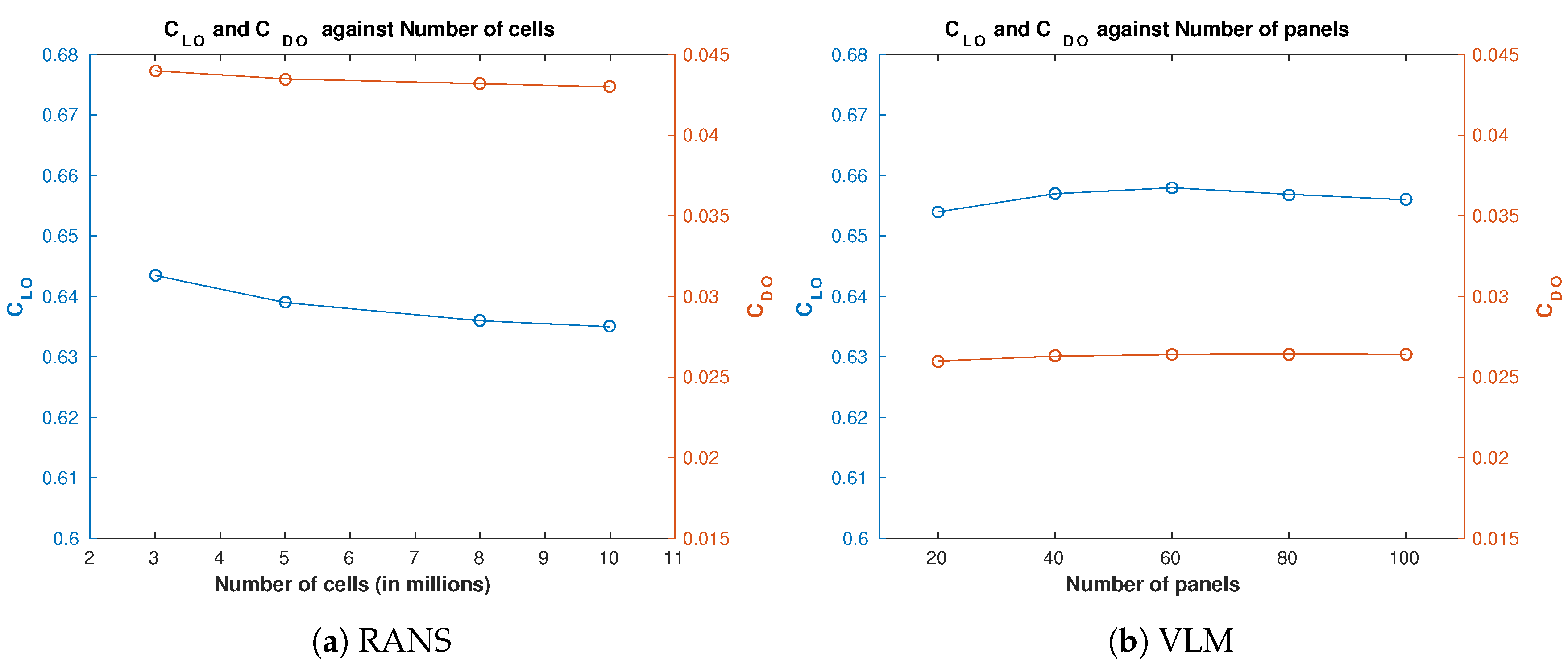
2.2. High-Fidelity: Reynolds Averaged Navier-Stokes

The high-fidelity approach considered is the RANS method in three spatial dimension. The RANS equations describe time-averaged motion of fluid flow through a control volume. The instantaneous physical quantities are decomposed into their time-averaged and fluctuating parts. The flow considered in the present computations involves the NACA23012 configuration at a Reynolds number of $Re=0.24\times {10}^6$ based on the wing’s chord length, corresponding to a fully turbulent regime. As the flow test cases considered for this work are below the compressibility limit, steady state solutions are obtained by solving the incompressible RANS equations; the system of equations expressing mass and momentum conservation within a finite controlled volume are written as in Equation (11).

$$\begin{array}{cc}\hfill \frac{\partial {\mathit{u}}_i}{\partial x_i}& =0\hfill \\ \hfill \frac{\partial \left(\rho {\mathit{u}}_i{\mathit{u}}_j\right)}{\partial x_j}& =-\frac{\partial p}{\partial x_i}+\frac{\partial {\mathit{\tau }}_{ij}}{\partial x_j}\hfill \end{array}$$

(11)

where ${\mathit{u}}_i$, ${\mathit{\tau }}_{ij}$ and p are the velocity vector, the shear stress tensor and the pressure, respectively. The SST $\kappa -\omega$ turbulence model is considered for modelling the viscous turbulent stresses. The model is based on the shear–stress–transport (SST) formulation which blends the $\kappa -\omega$ [22] and $\kappa -ϵ$ [23] turbulence models. The $\kappa -\omega$ model is well suited to model the flows inside the viscous sub-layer and and $\kappa -ϵ$ model is understood to be good at predicting flows in the regions away from the wall [24].

The CFD model is completed with the generation of three-dimensional grids with frontal radius and downstream length of 200 and 500 chord lengths, respectively, as shown in Figure 4. Hybrid meshes are generated comprising of a quadrilateral dominant surface grid for both wings. A hexahedral inflation layer is wrapped around each wing to capture the boundary layer up to the sub-viscous region maintaining a $y^{+}\approx 1$. Figure 5 demonstrates the different focus angles of the cut-section volume grid close to the wing as well as the refinement region in the wake. The far-field fluid domain is filled with unstructured tetrahedral cells with varying spatial resolution to capture the flow exhibiting strong gradients near and around the surfaces of wings.

3. Application of the Multi-Fidelity Framework

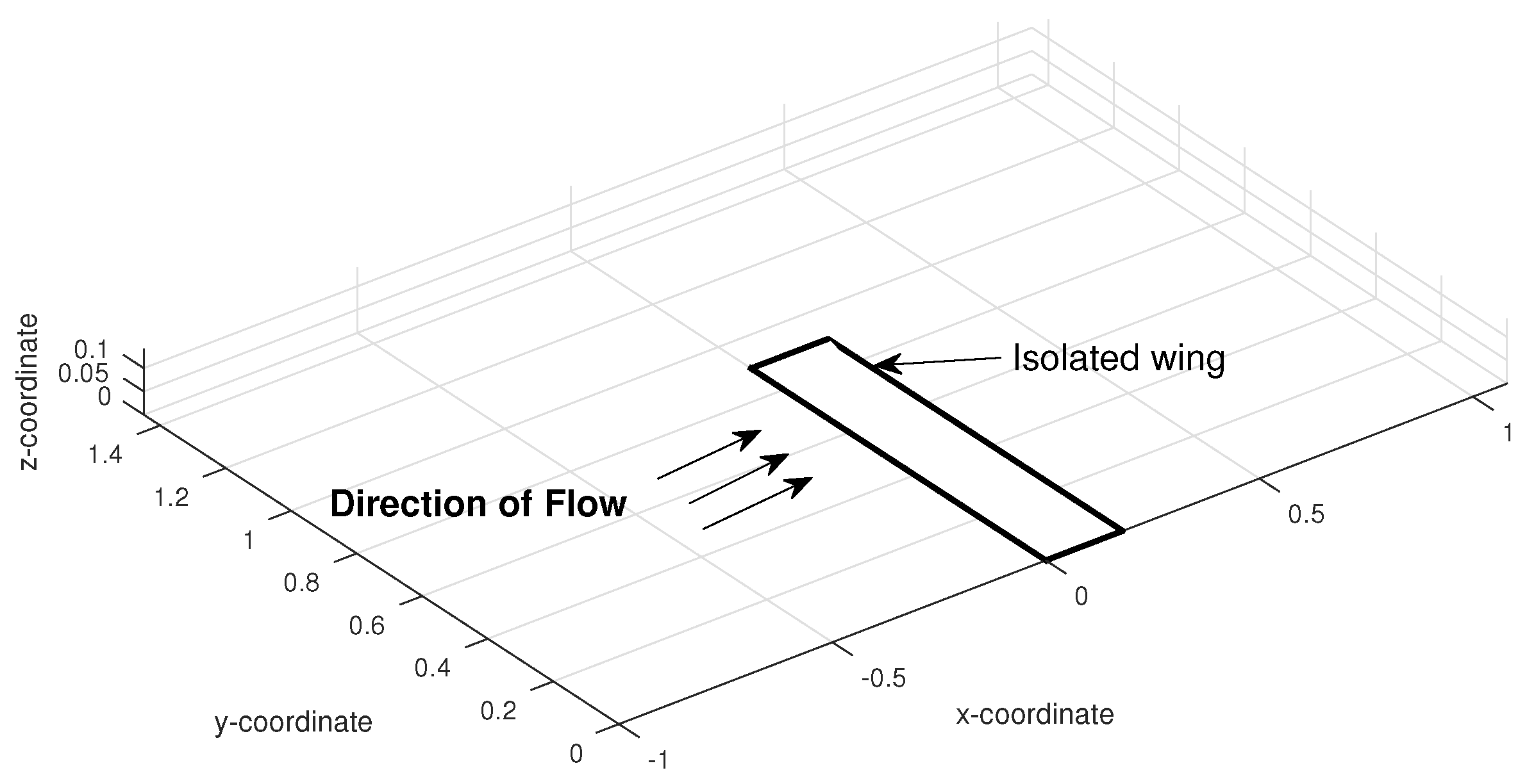
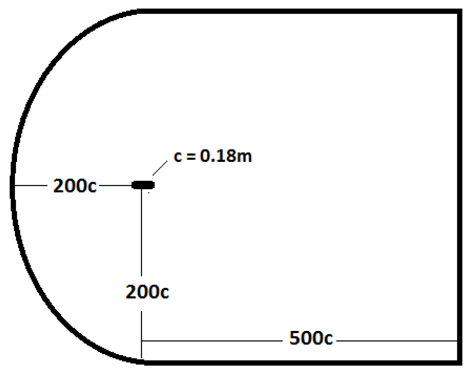
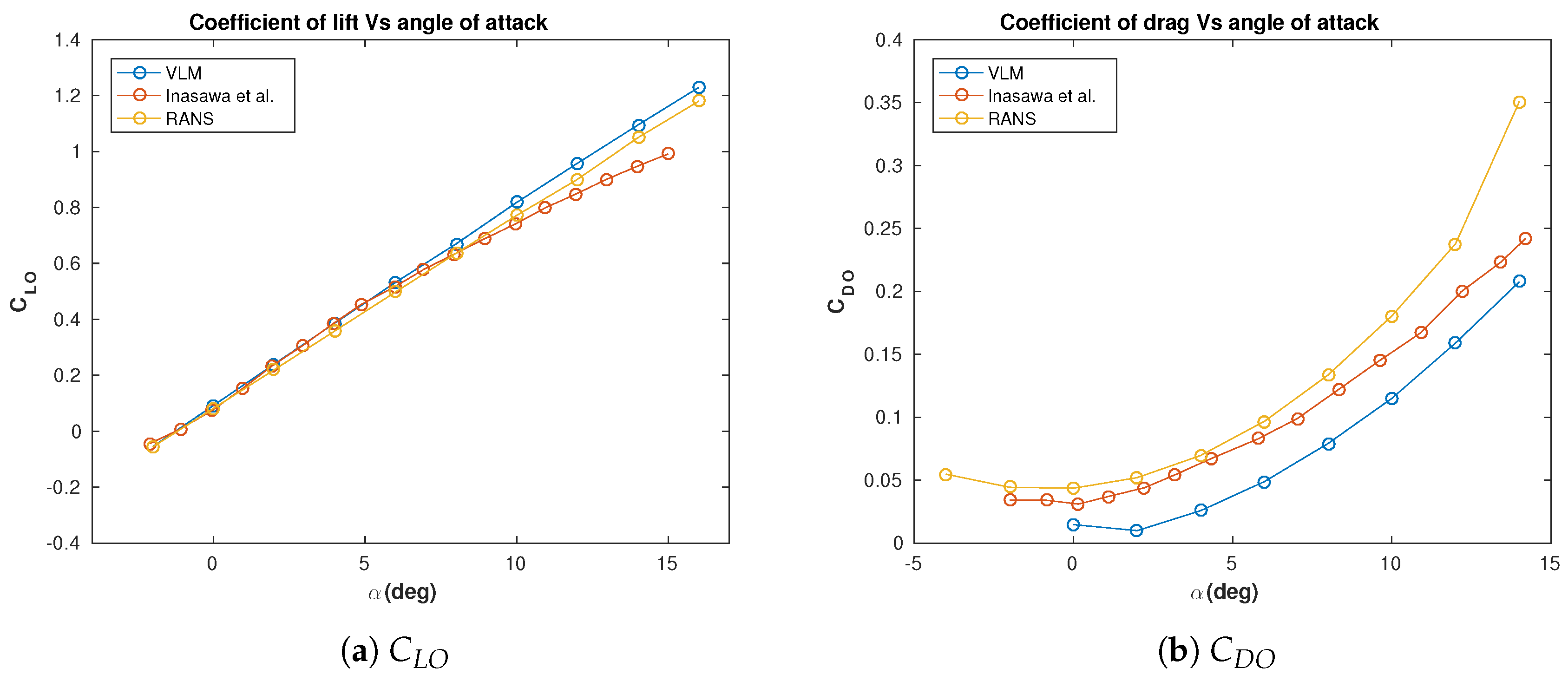
This section is divided in four subsections. Section 3.1 and Section 3.2 contain the verification procedure of the multi-fidelity framework, where RANS and VLM calculations are carried out for an isolated NACA23012 wing and for the same wing in double tandem configuration at $8^{\circ }$ angle of attack. The computed solutions are compared against wind-tunnel data. An analysis is carry-out where we investigate the effect of the leading wing’s angle of attack on the overall formation flight aerodynamic performance within Section 3.3. Finally, we demonstrate the flexibility aspects of the developed framework for blended wing formation configurations in Section 3.4.

3.1. Isolated Wing

Initially, an isolated wing configuration is considered which consists of a single NACA23012 wing at angle of attack of $AOA$ = $8^{\circ }$, which is shown in Figure 3 at corresponding Reynolds number of $Re=0.24\times {10}^6$ and a free-stream velocity of 20 m/s. The main objective of this analysis is to assess the accuracy and uncertainty levels of each of the computational fidelity approaches, i.e., VLM and RANS, and compare with experiment.

A numerical simulation is considered to be consistent when the numerical solution approaches the exact solution as the grid spacing tends to zero [25]. To study the effect of grid refinement for the RANS simulation on the solution accuracy, four meshes with increasing element count are generated with 3, 5, 8 and 10 million cells, for the isolated wing case. Similarly, the spatial resolution is also assessed for the VLM method, by computing the solution from 20 to 100 panels; for 100 panels, 5 in chordwise and 20 in spanwise direction are set. Lift ($C_{LO}$) and drag ($C_{DO}$) coefficients are plotted against the number of cells and number of panels for RANS and VLM in Figure 6. In the case of RANS, the change in $C_{LO}$ and $C_{DO}$ obtained from the 8 and 10 millions element meshes is less than $0.1\%$.

The lift coefficient ($C_{LO}$) and drag coefficient ($C_{DO}$) for an isolated NACA23012 wing are plotted against angle of attacks $AOA$ ranging from $-4^{\circ }$ to ${14}^{\circ }$ and compared against the experimental data from Inasawa et al. [10] in Figure 7. The $C_{LO}$ values obtained from VLM maintain a linear trend throughout the polar and superimpose the experimental data up to around $8^{\circ }$ incident. This demonstrates that the VLM method performs adequately well for small angles. Slight over-predictions become apparent with respect to the lift for angles greater than $8^{\circ }$ by the VLM estimations. With respect to the drag, VLM solutions are under-predicted throughout the polar; this is expected to some extent as the method is based on the inviscid, irrotational potential flow theory and accounts just for the lift-induced drag. RANS solutions are clearly more accurate and with smaller deviations from the experiment in terms of both drag and lift. The experimental lift to drag ratio ($L/D$) at $5^{\circ }$ angle of attack is $16.5$, whereas, for the RANS, the $L/D$ value turns out to be $14.93$ with an error of $9.5\%$. When compared against the VLM, RANS is conclusively more accurate at predicting the drag coefficient.

Both approaches demonstrated to be effective and reliable techniques for performing aerodynamic analysis with an error of under $5\%$ for $C_{LO}$ and of $11\%$ in the case of $C_{DO}$ up to ${11}^{\circ }$ angle incident. The computational effort required to run one VLM simulation with 200 panels is 30 s, as compared to 2.5 h for the RANS computation using open-foam, on a Intel Core i5-7600K processor, 4 CPUs, 12 GB of RAM, with the 8 million grid.

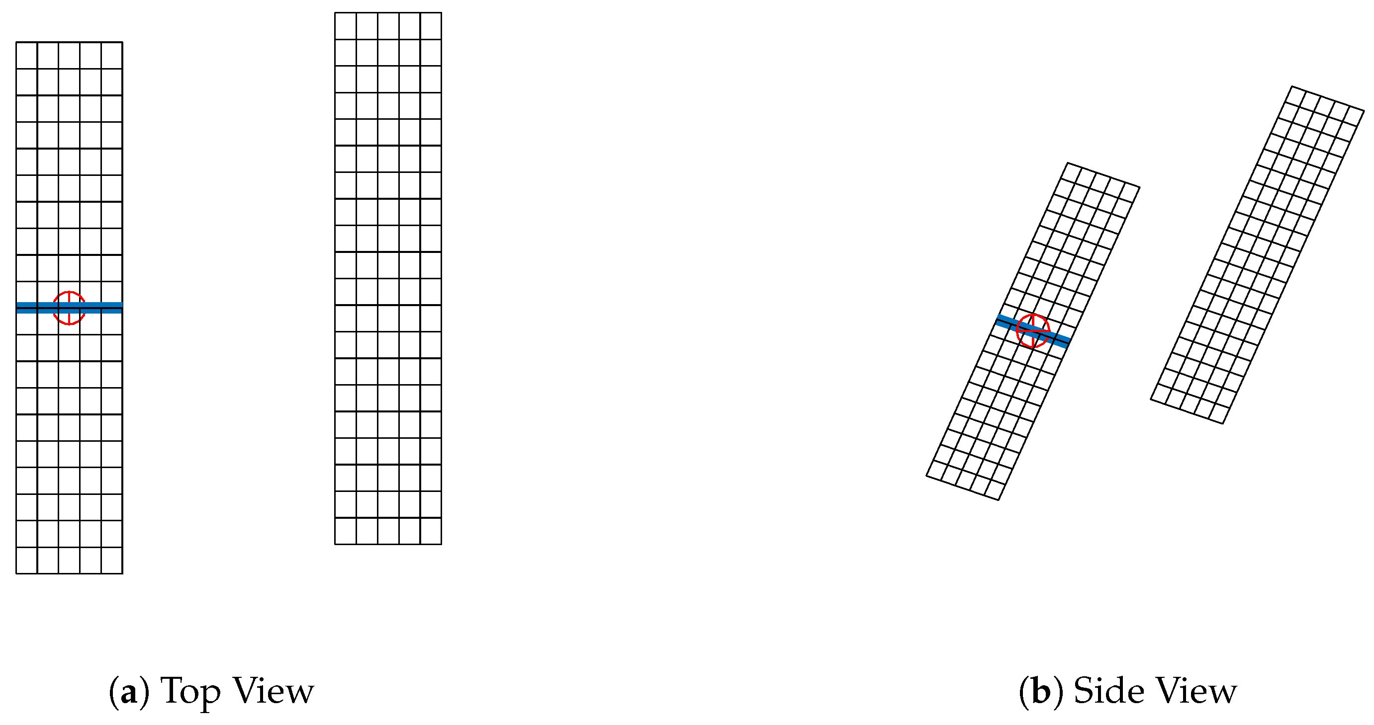
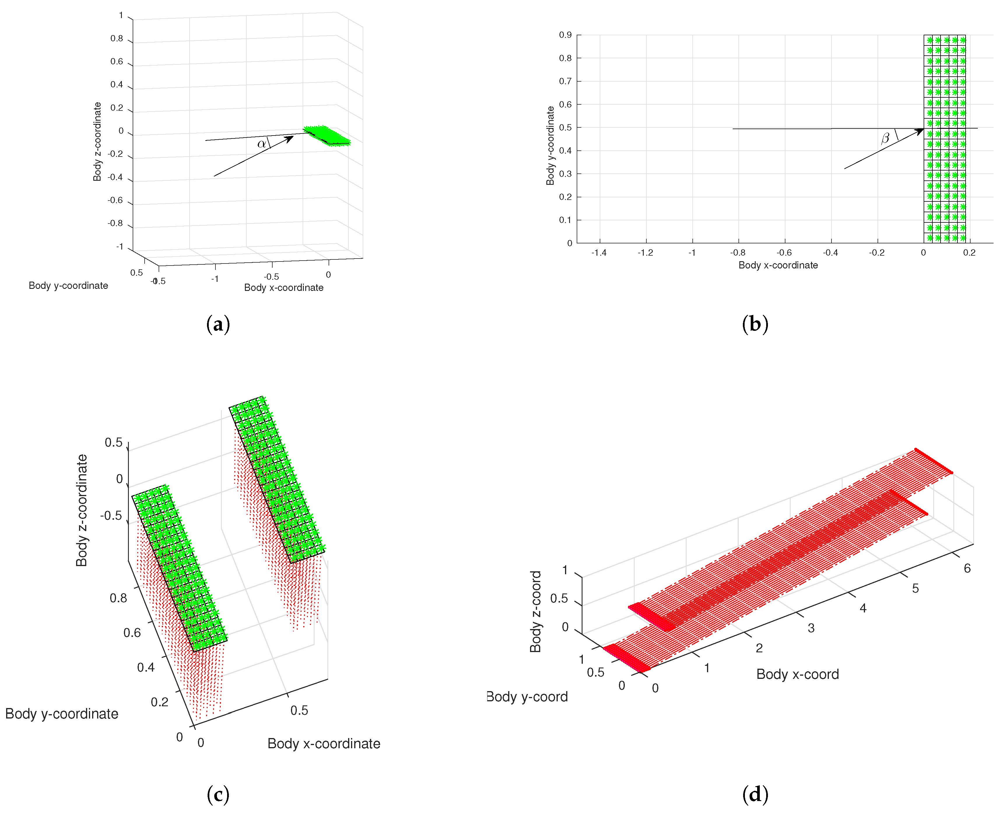
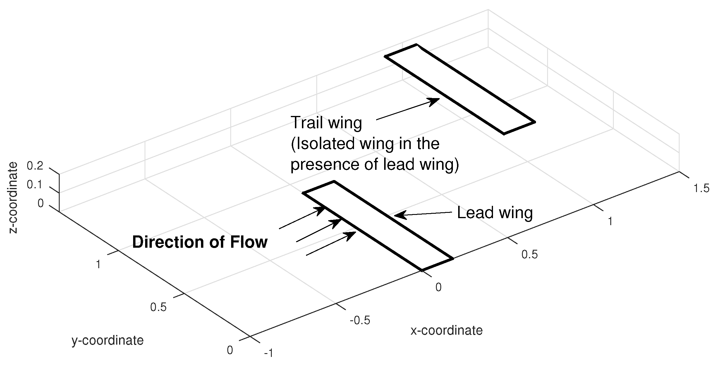
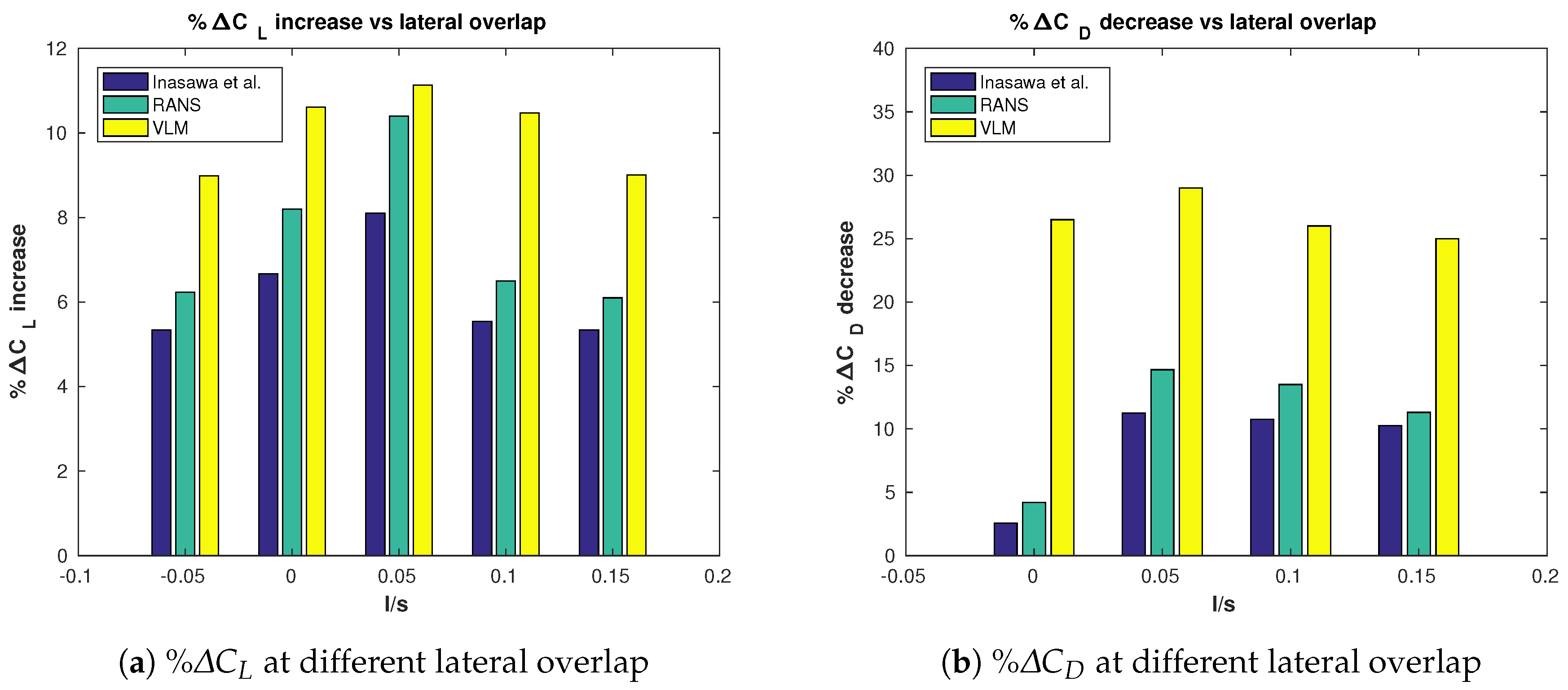
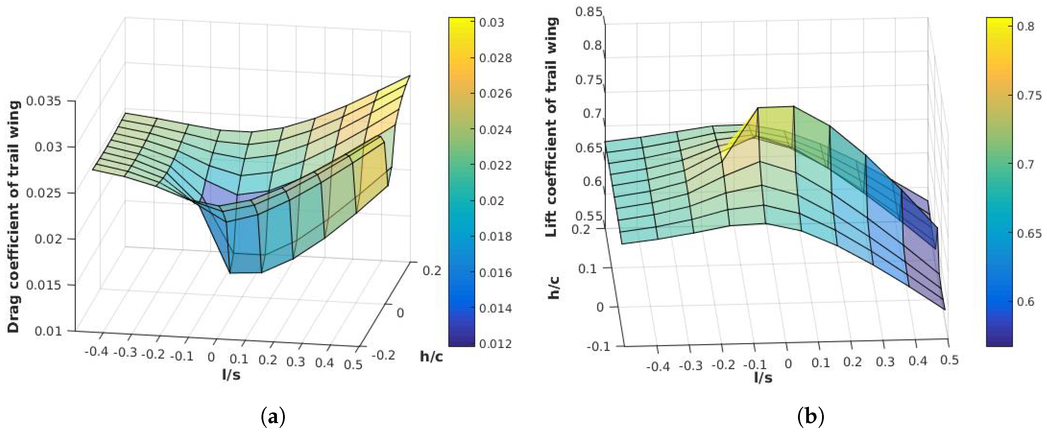
3.2. Two Wings in Tandem Configuration

An additional rectangular NACA23012 wing is introduced to the isolated wing configuration discussed in the previous section. For this section, the isolated wing is now referred to as trail wing in the two wing configuration, as depicted in Figure 8. This is done to directly compare the aerodynamic performance of the isolated wing to the same isolated wing in the wake region of the lead wing. By incorporating a second wing, the relative positioning and flight dynamics parameters (yaw, pitch and roll) are varied of each body to obtain the best aerodynamic performance in terms of total quantities, e.g., total drag reduction and lift over drag ratio. The position of the lead wing is held constant while the trail wing is allowed to move in the y-z plane at different stream-wise positions. Both the lead and the trail wings are set at incident angle of $AOA=8^{\circ }$; the freestream velocity is set to 20 m/s and a Reynolds number of $Re=0.24\times {10}^6$.

The displacement of the trail wing behind the lead wing is monitored by the given transformed coordinates as depicted in Figure 8 where the lateral displacement corresponds to ($l/s$), the vertical to ($h/c$) and the stream-wise direction at ($x/c$). Note that the $l/s$ is positive when the lead and the trail wing are in overlapping position. The aerodynamic performance gains are assessed by calculating the percentage change in the lift and drag coefficient of the trail wing ($C_L$ and $C_D$) in the presence of the lead wing compared against the lift and drag coefficient of an isolated configuration ($C_{LO}$ and $C_{DO}$). The aerodynamic performance is evaluated at the trail wing by VLM and RANS, and compared with experiment, it is appropriate to evaluate the percentage’s variation than the absolute values; thus the percentage change in lift and drag coefficients are calculated as $\%\Delta C_L=(C_L-C_{LO})/C_{LO}$ and $\%\Delta C_D=(C_{DO}-C_D)/C_{DO}$. Note that the change between the isolated and trail wings is monitored in percentages. This implies that at the optimum position, the trail wing is expected to have maximum increase in lift and maximum decrease in drag. Moreover, it is further to be noted that, in the expressions for $\%\Delta C_L$ and $\%\Delta C_D$, the terms representing the respective quantities for the isolated and the trail wings are switched. This is to keep consistency with the expressions detailed in the experimental analysis.

Figure 9 demonstrates the performance of the percentage variations of lift and drag, $\%\Delta C_L$ and $\%\Delta C_D$, at five lateral overlapping positions $l/s=-0.05,0,0.05,0.01$ and $0.15$, solutions from VLM and RANS are compared with experiment. RANS and VLM over-predict the $\%\Delta C_L$ values for $l/s=0.05$ with an error of $13\%$ and $18\%$, respectively, compared with reference data.

The RANS computations suggest a negative overlapping position ($l/s=-0.05$) where the $\Delta C_D$ attains the minimum value of $5\%$ as shown in Figure 9b. As the wing overlap becomes positive ($l/s=0$ to $0.05$), the $\Delta C_D$ value increases from $9\%$ to maximum value of $11\%$ with an error of $17\%$. By plugging in a span value of 0.9 units in the formula given by Hummel [5] discussed in Section 1, the optimum wing tip overlap value ($l/s$) turns out to be 0.0495 units which translates to around $l/s=0.05$. This overlapping position in fact marks the position for maximum decrease in $\Delta C_D$ values for both the experiment $(8\%)$ and the RANS $(9.3\%)$ with an error of $16.25\%$. Same degree of error is observed in deeper overlapping positions i.e., at $l/s=0.1$ and $0.15$ where both the $\Delta C_L$ and $\Delta C_D$ values start to decrease as compared to the optimum lateral overlapping position of $l/s=0.05$. This is attributed to the fact that, along with the upwash, the downwash from the lead wing vortex also acts on the trail wing thereby offsetting the upwash, resulting in decreased aerodynamic performance.

For the VLM solutions, drag over-predictions are observed at all the discrete locations by almost 20–25% when compared against experimental values. Maximum value of $\Delta C_L$ is also observed at $l/s=0.05$ position, as shown in Figure 10a,b, where the absolute values of lift and drag of trailwing are plotted as a response surface of the $h/c$ and $l/s$ displacement variables. It is also noted that the maximum drag reduction predicted by the VLM occurs at the same location and is as large as $27\%$ in magnitude as compared to $10\%$ in the case of experiment. Such high values of drag reductions are often cited by the various researchers undertaking computational analysis based on potential flow theory. Iglesis and Mason [26] used the discrete vortex method and concluded that the drag reductions of $30\%$ for formation of three aircraft is achievable with central aircraft as the leader.

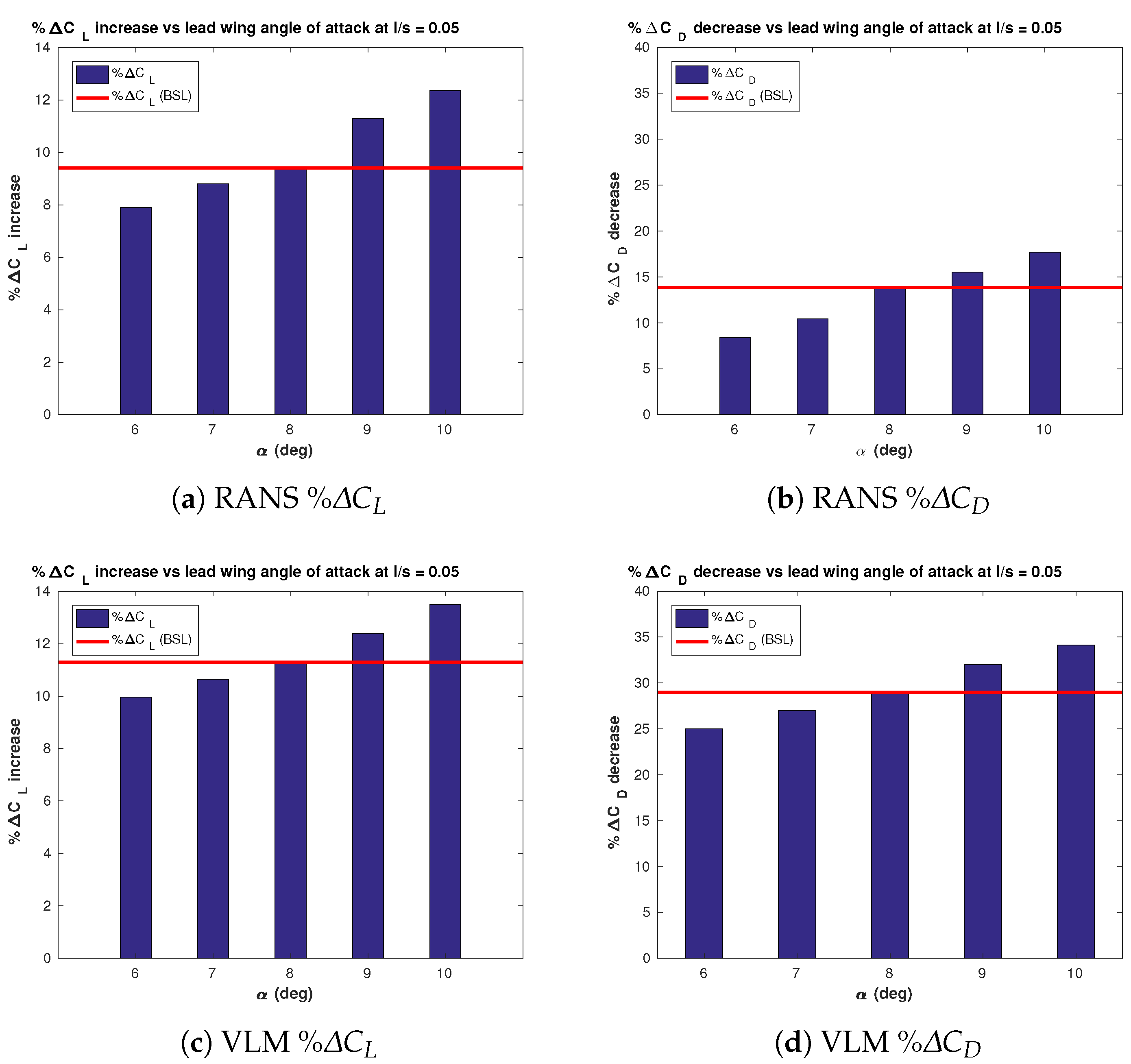
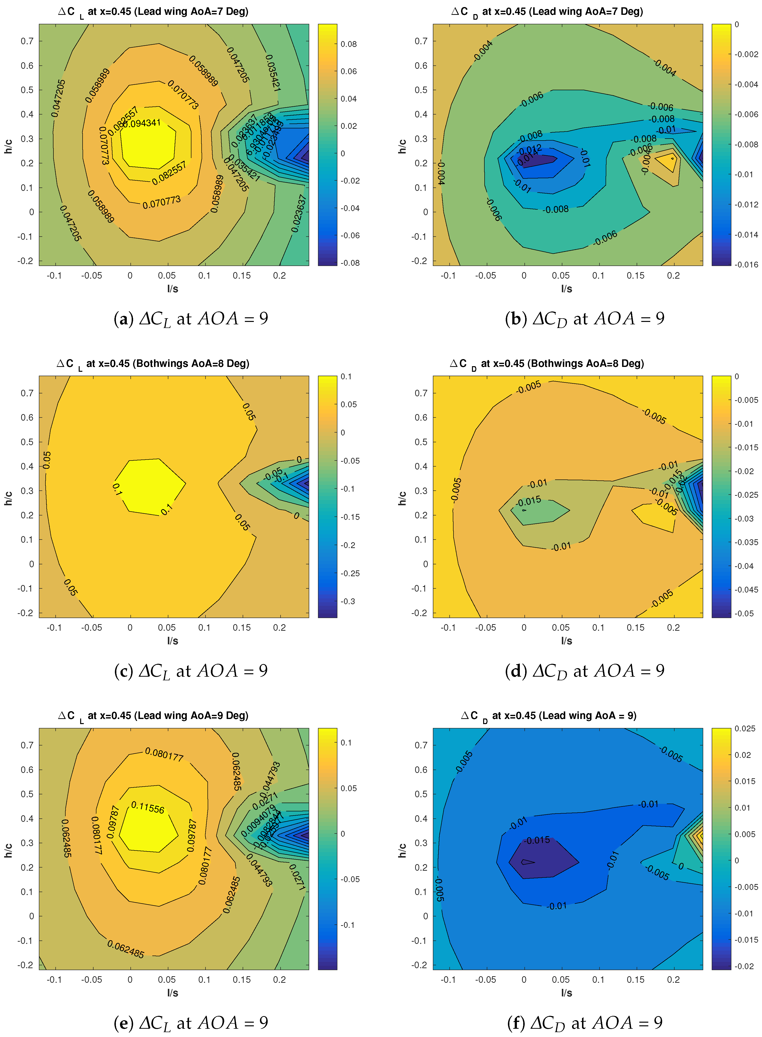
3.3. Effect of the Lead Wing’s AOA

Increasing the angle of attack can be favourable as the induced lift is increased, stronger pressure gradient would be present in the vicinity of wingtip vortices. This is attributed to the higher pressure difference between the upper and lower surfaces of the wing, which provides a more energetic upwash for the trailing wing. Therefore, this section is devoted to the assessment of the effect of the leading wing’s angle of incident to the overall aerodynamic performance of the system. The angle of the lead wing is varied from $6^{\circ }$ to ${10}^{\circ }$ keeping the trail wing angle constant at $8^{\circ }$. When both wings are set at $8^{\circ }$ angle, the configuration is referred to as baseline configuration (BSL). The setup for these computations is identical as described in the previous Section 3.2 with the exception that lead wing’s AOA is varied. Results obtained from RANS and VLM are compared against the baseline configuration prediction of the previous section. The analysis is restricted within the linear range as higher angles might lead to larger discrepancies particularly for the low-fidelity solver as boundary layer separation might be present [27].

It is observed in Figure 11 that for both techniques at the trail wing’s $\Delta C_L$ values share a linear relationship with the lead wing’s angle of attack when compared against the results obtained from the baseline configuration. In the case of the RANS predictions, there is an increase in $\Delta C_L$ value of $10\%$ for the trail wing compared to $6\%$ in the case of the experiment. The $\Delta C_L$ of the trail wing drops to $8\%$ when lead wing’s angle is at $6^{\circ }$, whereas it increases to $12\%$ at ${10}^{\circ }$, as shown in Figure 11a. Figure 11c shows similar trend in the case of the VLM but with slight increase in the magnitude of $\Delta C_L$ values for all the incidence angles. The $\Delta C_D$ values are over predicted by almost twice, as observed in the case of RANS. It can been noted that the low-fidelity prediction for all angles, predict the expected increase in lift and also the increase in absolute values of $\Delta C_D$ are in comparable range as seen in Figure 11d.

The aerodynamic performance predictions obtained from the VLM solver are plotted in terms of $\Delta C_L$ and $\Delta C_D$ with colour contours at different lead wing’s angles at 7, 8 and 9 in Figure 12. It can be noted that, for all three lead wing’s angles, there is no substantial benefit from the upwash created by lead wing’s vortices beyond $13\%$ lateral overlap marked by contours in the blue colour region. As the lateral overlap ($l/s$) is further increased, $\Delta C_L$ values become negative indicating that an isolated wing has greater lift coefficient than the trail wing in the presence of the lead wing, as the trail wing is in the pronounced downwash region created by the lead wing. It is also noted that the maximum increase in $\Delta C_L$ and maximum decrease in $\Delta C_D$ values are observed between the overlapping positions $l/s=0$ to $l/s=0.05$. Furthermore, as shown in Figure 12a,c,e, the regions pronouncing the best aerodynamic performance “sweet spot” of the trail wing shift upwards as the angle is increased to $9^{\circ }$ and drops down when is reduced to $7^{\circ }$ when compared against the baseline configuration. This is mainly because the wake in the VLM is parallel to the free-stream direction, whereas, in the real flows, the self induced velocities cause the longitudinal position of the vortex to drop in longitudinal direction.

The qualitative analysis of $\Delta C_D$ contours shown in Figure 12b,d,f reflect somewhat the same position for the maximum drag reduction. As can be seen in Figure 11, VLM predicts as much as $30\%$ increase in induced drag component at higher AOA. Even though the quantification of drag reduction does not yield reliable replication of the experimental values yet, it proves to be of immense importance when used in conjunction with the $\Delta C_L$ contours to study various variables in formation flights for relatively lower computational expense method. The multi-fidelity approach i.e employing VLM approach at early stages of analysis clearly proves prudent in deciphering the main flow features and general quantification of the aerodynamic coefficients at early stages of the analysis provide good insight of the design changes required for a particular requirement. This inexpensive approach helps in downsizing the simulation space for high-fidelity computation in the final stages of a computational analysis.

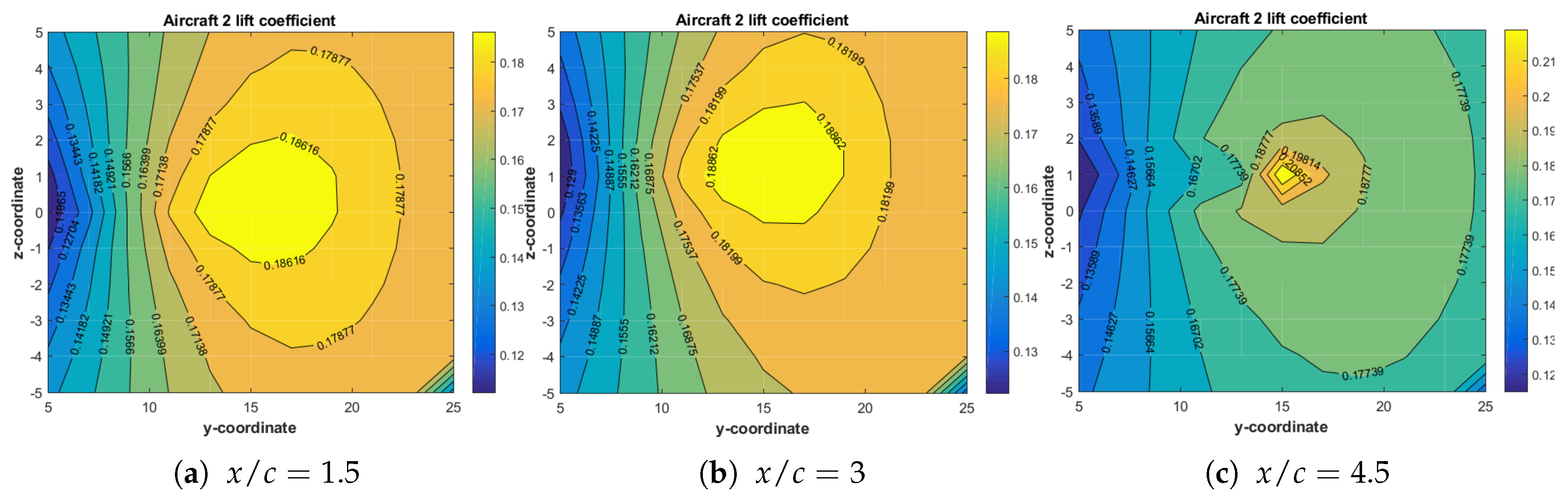
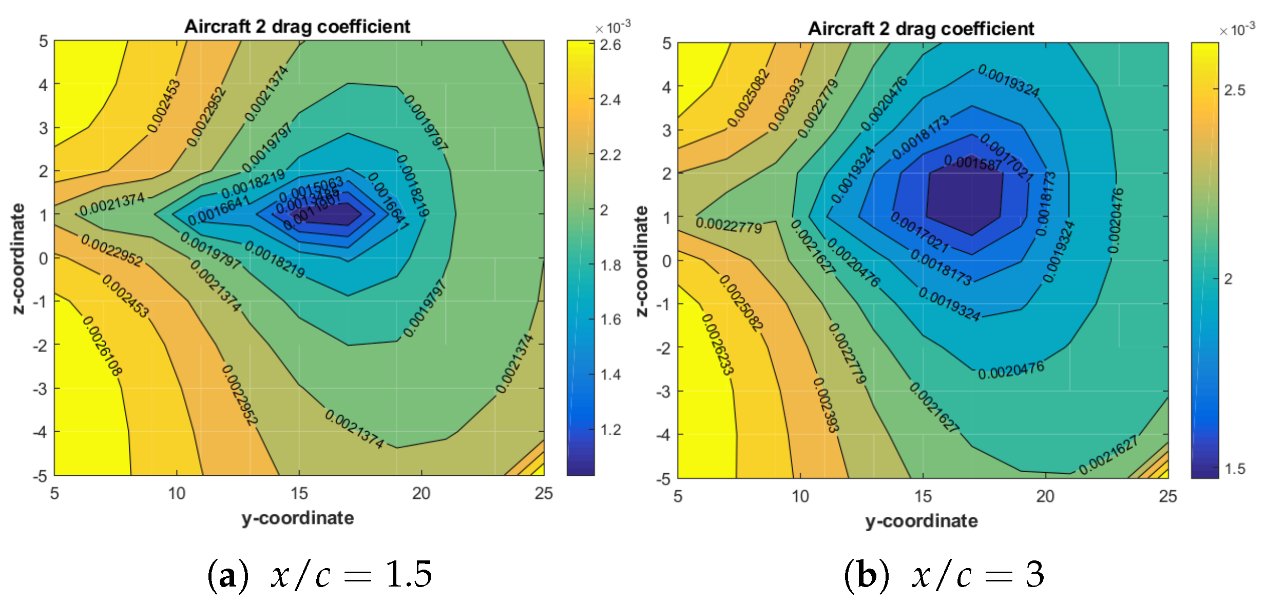
3.4. Blended-Wing-Body Aircraft in Formation

We extend the application of multi-fidelity approach to a realistic aircraft formation of a blended-wing-body aircraft configuration in formation. The main objective is to assess the flexibility of the developed framework. The flight conditions are set as steady level flight at a free-stream Mach number of 0.3, at an angle of attack of 3${}^{\circ }$ with a corresponding Reynolds number of $\left(Re\right)=40\times {10}^6$ based on the mean aerodynamic chord of $mac=6.6$ m.

Initially, an isolated blended-wing-body configuration is modelled to determine the panel and grid sensitivity on the solutions. Figure 13 shows the lift and drag coefficient estimates for panel and RANS approaches; it can be noted that monotone behaviours are observed and an obvious trend for grid/panel independence for both methods, at approximately 800 panels and 6 million elements for VLM and RANS, respectively. The setup of the RANS computations is similar to in the previous section including the meshing strategy, numerical scheme and turbulence model, whereas the incompressible steady state RANS equations are solved and discretised by a second-order upwind method and turbulence effects are accounted with the $\kappa -\omega$$SST$ model.

A two aircraft configuration is considered. The distribution of the quadrilateral panels and triangular surface elements for the configuration in depicted in Figure 14. Note, for the low-fidelity VLM approach, thin surfaces are considered.

The procedure for determining the optimum position of the second aircraft to maximise the overall aerodynamic performance is set by fixing the lead aircraft and displacing the trailing aircraft in the Cartesian reference frame. With respect to y-z plane, a increment of $\delta y/c=0.15$ and $\delta z/c=0.075$ and three free-stream locations at $x/c=1,3$ and $4.5$ are set, as shown in Figure 15.

Figure 15 shows the lift of the second aircraft obtained by the VLM solver, with the second aircraft at three stream-wise ($x/c$) locations. The plots suggest that the highest lift is achieved at 11% wing-tip overlap of the aircraft and at lower $x/c$ distance. Figure 16 shows the drag coefficient, in which it can be seen that the point of the highest drag coefficient drop, optimal position for aerodynamic improvement, is at the coordinates $x/c=1.5$, $y/c=2.5$ and $z/c=0.15$. The drag coefficient is $0.0016$ which suggests $30\%$ reduction in drag as compared to an isolated aircraft. The overlap distance between the two wing-tips is about 10.2% of the aircraft span. When the overlapping positioning of the two aircraft increases, the drag also increases and the lift starts to drop. This is mainly because, in this region, the trail aircraft is under a direct influence of just the downwash created by the lead wing and hence no aerodynamic performance improvements are encountered.

High-fidelity computations are performed at the optimum solution suggested by the VLM with the second aircraft positioned at $x/c=1.5$, $y/c=2.5$ and $z/c=0.15$. The high-fidelity solutions predict a drag coefficient of 10% higher than the VLM estimation, as shown in

Table 1. Drag and lift coefficients for isolated and trail aircraft in formation for the blended-wing-configuration at optimal position.

Configuration	Aerodynamic Coefficients	VLM	RANS
Isolated aircraft	$C_D$	0.0022	0.0028
	$C_L$	0.1758	0.1290
Trail aircraft in formation	$C_D$	0.0016	0.0019
	$C_L$	0.1935	0.1450

. Note also that a 5% reduction in drag is obtained compared to the isolated aircraft at the same coordinate position. The “sweet spot”, which marks the location for the maximum drag reduction for the trail wing behind the lead wing, is found to be around $10\%$ wing-tip overlap for both VLM and the RANS.

4. Conclusions

A novel computational framework is proposed to determine flight formation and analyse the aerodynamic performance benefits using a multi-fidelity approach. The multi-fidelity approach for this study is based on a low-fidelity, Vortex Lattice Method and a high-fidelity, Reynolds Averaged Navier–Stokes solver. The developed modules for the low-fidelity solver are validated against the high-fidelity and experimental measurements on two distinct flow cases.

Initially, a rectangular wing NACA23012 is considered to validate the numerical framework; the main aim is to determine and to quantify the accuracy of each method. Two NACA23012 are considered in tandem configuration; the relative position of the second wing is altered at various longitudinal, horizontal and vertical positions. Computations are performed with both fidelity approaches and compared with wind-tunnel measurements [10]. The low-fidelity solver over-predicts lift and drag value compared with the available experiment, however the experiment and both fidelity solvers predict the same location of minimum drag and maximum lift. Moreover, the effect of lead’s wing angle of attack on the two wing aerodynamic performance is studied by considering three angles within the linear range. It was found that no considerable variation of the lateral and vertical position occurs for maximum aerodynamic performance for these three angles. The last test case considered is the flow over a blended-wing-aircraft configuration; the multi-fidelity framework is employed to determine the best aerodynamic position of the trail aircraft, and a drag reduction of 30% is achieved, which agrees with similar studies. The developed multi-fidelity framework forms the basis for aerodynamic performance estimation of larger formation flights (<3 bodies) and the robust data generation tool for future multi-objective optimisation analyses.

References

1. Weimerskirch, H.; Martin, J.; Clerquin, Y.; Alexandre, P.; Jiraskova, S. Energy saving in flight formation. Nature 2001, 413, 697–698. [Google Scholar] [CrossRef] [PubMed]
2. Bajec, I.; Heppner, F. Organized flight in birds. Anim. Behav. 2009, 78, 777–789. [Google Scholar] [CrossRef]
3. Lissaman, P.; Shollenberger, C.A. Formation flight of birds. Science 1970, 168, 1003–1005. [Google Scholar] [CrossRef] [PubMed]
4. Hainsworth, F.R. Precision and dynamics of positioning by Canada geese flying in formation. J. Exp. Biol. 1987, 128, 445–462. [Google Scholar]
5. Beukenberg, M.; Hummel, D. Aerodynamics, Performance and Control of airplanes in formation flight. In Proceedings of the 17th Congress of the International Council of the Aeronautical Sciences, Stockholm, Sweden, 9–14 September 1990; Volume 2, pp. 1777–1794. [Google Scholar]
6. DeVries, L.D.; Paley, D.A. Wake estimation and optimal control for autonomous aircraft in formation flight. In Proceedings of the Conference on AIAA Guidance, Navigation, and Control (GNC), Boston, MA, USA, 19–22 August 2013; p. 4705. [Google Scholar]
7. Shin, H.; Antoniadis, A.; Tsourdos, A. Parametric Study on Formation Flying Effectiveness for a Blended-Wing UAV. J. Intell. Robot. Syst. 2018, 10. [Google Scholar] [CrossRef]
8. Qiu, H.; Duan, H. Multiple UAV distributed close formation control based on in-flight leadership hierarchies of pigeon flocks. Aerosp. Sci. Technol. 2017, 70, 471–486. [Google Scholar] [CrossRef]
9. Pahle, J.; Berger, D.; Venti, M.; Duggan, C.; Faber, J.; Cardinal, K. An initial flight investigation of formation flight for drag reduction on the C-17 aircraft. In Proceedings of the AIAA Atmospheric Flight Mechanics Conference, Minneapolis, MN, USA, 13–16 August 2012; pp. 13–16. [Google Scholar]
10. Ayumu Inasawa, F.M.; Asai, M. Detailed Observation of Interaction of Wingtip Vortices in Close-formation Flight. J. Aircr. 2012, 49, 206–213. [Google Scholar] [CrossRef]
11. Blake, W.; Gingras, D.R. Comparison of predicted and measured formation flight interference effects. J. Aircr. 2004, 41, 201–207. [Google Scholar] [CrossRef]
12. Slotnick, J.P.; Clark, R.W.; Friedman, D.M.; Yadlin, Y.; Yeh, D.T.; Carr, J.E.; Czech, M.J.; Bieniawski, S.W. Computational aerodynamic analysis for the formation flight for aerodynamic benefit program. In Proceedings of the 52nd Aerospace Sciences Meeting, National Harbor, MD, USA, 13–17 January 2014; AIAA Paper. p. 1458. [Google Scholar]
13. Ning, A.; Flanzer, T.C.; Kroo, I.M. Aerodynamic performance of extended formation flight. J. Aircr. 2011, 48, 855–865. [Google Scholar] [CrossRef]
14. Blake, W.; Multhopp, D. Design, Performance and Modeling Considerations for Close Formation Fligh. In Proceedings of the 23rd Atmospheric Flight Mechanics Conference, Boston, MA, USA, 10–12 August 1998. AIAA Paper 98-4343. [Google Scholar]
15. Maskew, B. Formation Flying Benefits Based on Vortex Lattice Calculations; NASA CR-151974; NASA: Washington, DC, USA, 1977. [Google Scholar]
16. Wagner, E.; Jacques, D.; Blake, W.; Pachter, M. Flight test results of close formation flight for fuel saving. In Proceedings of the AIAA Atmospheric Flight Mechanics Conference and Exhibit, Monterey, CA, USA, 5–8 August 2002. [Google Scholar]
17. Wagner, H.E. An Analytical Study of T-38 Drag Reduction in Tight Flight Formation. Air Force Inst of Tech Wright-patterson Afb oh School of Engineering and Management. In Proceedings of the Atmospheric Flight Mechanics Conference, Denver, CO, USA, 14–17 August 2000. [Google Scholar]
18. Korkischko, I.; Konrath, R. Formation Flight of Low-Aspect-Ratio Wings at Low Reynolds Number. J. Aircr. 2016, 54, 1025–1034. [Google Scholar] [CrossRef]
19. Thien, H.; Moelyadi, M.; Muhammad, H. Effects of leaders position and shape on aerodynamic performances of V flight formation. arXiv, 2008; arXiv:0804.3879. [Google Scholar]
20. Gunasekaran, M.; Mukherjee, R. Behaviour of trailing wing(s) in echelon formation due to wing twist and aspect ratio. Aerosp. Sci. Technol. 2017, 63, 294–303. [Google Scholar]
21. Melin, T. A Vortex Lattice MATLAB Implementation for Linear Aerodynamic Wing Applications. Master’s Thesis, Department of Aeronautics, Royal Institute of Technology (KTH), Stockholm, Sweden, 2000. [Google Scholar]
22. Wilcox, D. Formulation of the kappa-omega turbulence model revisited. AIAA J. 2008, 46, 2823–2838. [Google Scholar] [CrossRef]
23. Chien, K. Predictions of channel and boundary-layer flows with a low-reynolds-number turbulence model. AIAA J. 1982, 20, 33–38. [Google Scholar] [CrossRef]
24. Menter, F.R. Two-Equation Eddy-Viscosity Turbulence Models for Engineering Applications. AIAA J. 1994, 32, 1598–1605. [Google Scholar] [CrossRef]
25. Roache, P.J.; Ghia, K.N.; White, F.M. Editorial policy statement on the control of numerical accuracy. J. Fluids Eng. 1986, 108. [Google Scholar] [CrossRef]
26. Iglesias, S.; Mason, W. Optimum spanloads in formation flight. In Proceedings of the 40th AIAA Aerospace Sciences Meeting & Exhibit, Reno, NV, USA, 14–17 January 2002; AIAA Paper. Volume 258. [Google Scholar]
27. Ekaterinaris, J.; Platzer, M. Computational prediction of airfoil dynamic stall. Prog. Aerosp. Sci. 1998, 33, 759–846. [Google Scholar] [CrossRef] [Green Version]
Figure 1. Panel distribution on rectangular wings.
Aerospace 05 00066 g001
Figure 2. (a) Normal vectors (in red) and collocation points on wing surface (green); (b) free-stream wake of the lifting surface; (c) schematic of angle of attack ( α ) with arrow showing the direction of free-stream velocity (isometric view); and (d) schematic of angle of side-slip ( β ) with arrow showing the direction of free-stream velocity (plan-view).
Aerospace 05 00066 g002
Figure 3. Schematic of isolated wing NACA23012 and spatial domain within the VLM solver.
Aerospace 05 00066 g003
Figure 4. Topology and dimensions of spatial domain for RANS computations of NACA23012 case.
Aerospace 05 00066 g004
Figure 5. Cut-section of the 3D grids: (a) close-up of both wings; and (b) overview of both wings and grid refinement in the wake region.
Aerospace 05 00066 g005
Figure 6. Spatial resolution study for the isolated NACA23012 wing at 8 angle of attack, in terms of lift ( C L O ) and drag ( C D O ) coefficients for RANS and VLM methods.
Aerospace 05 00066 g006
Figure 7. Polar analysis of isolated NACA23012 wing plotting for coefficient of lift ( C L O ) and drag ( C D O ); results include VLM, RANS and experiment from Inasawa et al. [10].
Aerospace 05 00066 g007
Figure 8. Schematic of two NACA23012 wings in tandem configuration.
Aerospace 05 00066 g008
Figure 9. Percentage variations of drag ( % Δ C D ) and lift ( % Δ C L ) at five different displacements; solutions are shown for RANS and VLM and compared with the experimental data [10].
Aerospace 05 00066 g009
Figure 10. Three-dimensional response surfaces of absolute quantities against relative positions: (a) drag coefficient; and (b) lift coefficient, for VLM solutions.
Aerospace 05 00066 g010
Figure 11. Effect of lead wing’s AOA on aerodynamic coefficients of trail wing with red line corresponding to Baseline Configuration (Both wings A O A = 8): (a) percentage lift coefficient ( % Δ C L ) for RANS; (b) percentage drag coefficient ( % Δ C D ) for RANS; (c) percentage lift coefficient ( % Δ C L ) for VLM; and (d) percentage drag coefficient ( % Δ C D ) for VLM.
Aerospace 05 00066 g011
Figure 12. Contours of lift ( Δ C L ) and drag coefficient ( Δ C D ) percentage change for three lead wing incidence angles at streamwise distance of x = 0.45.
Aerospace 05 00066 g012
Figure 13. Grid/Panel dependence analysis for the isolated blended-wing-body aircraft configuration.
Aerospace 05 00066 g013
Figure 14. Panel distribution and surface gird distribution on the blended-wing-body two-aircraft configuration.
Aerospace 05 00066 g014
Figure 15. Lift coefficient contours of blended-wing-body configuration in double tandem formation flight of the trailing aircraft on y-z plane at three different stream-wise positions.
Aerospace 05 00066 g015
Figure 16. Drag coefficient contours of blended-wing-body configuration in double tandem formation flight of the trailing aircraft on y-z plane at two different stream-wise positions.
Aerospace 05 00066 g016