On the Choice of the Discount Rate and the Role of Financial Variables and Physical Parameters in Estimating the Levelized Cost of Energy

Abstract

The levelized cost of energy (LCOE) approach has become popular, especially in the field of renewable energy. We argue that when assessing levelized cost of energy, different rates should be used for borrowing and discount rates. We further argue that the risk-free rate should be used for discounting when assessing and comparing the cost of energy across different producers and technologies. Recent analyses used the same rate for borrowing and discounting, which leads to underestimation of the cost for risky borrowers and to distorted sensitivities of the cost to financial and non-financial factors. Specifically, it is shown that they may lead to gross underestimation of the importance of solar-to-electricity conversion efficiency when applied to photovoltaics. The importance of device efficiency is re-established under the treatment of the discount rate proposed here.

1. Introduction

Realistic estimates of the costs of energy from emerging energy generation technologies such as large-scale photovoltaic (PV) installations are necessary to guide rational resource allocation and to create a viable PV industry [1]. They are also important to help establish research priorities. This is all the more important, as achievable costs are still significantly higher than those for hydro, nuclear, coal, and gas powered electricity [2]. The advent of new drilling technologies and the concomitant collapse of natural gas prices in North America in recent years [3], the achievement of economical recoverability of vast deposits of oil in Canada [4] and of new deposits in South and Central America [5], coming at a time of strained public finances around the developed world set the bar for renewable energy and PV in particular higher today than was the case just a few years ago, as policy-makers may become less willing to renew or extend subsidies. It is therefore critical to develop quantitative methods for realistic assessment of costs. Recently, progress has been made in establishing a quantitative methodology to estimate such costs [2,6,7], and the levelized cost of energy (LCOE) has been widely used for that purpose by researchers and policymakers alike [8]. The LCOE approach computes the constant unit cost (e.g., per kWh) from the present value of costs incurred over the lifetime of the plant. Namely, the present discounted value of energy produced times the levelized cost equals the present discounted value of the fixed and variable costs over the life of the investment:

(1)

where Q_n and C_n are, respectively, the amount of energy produced and outlays in year n and DR is the discount rate.

Uncertainties surrounding the values of input parameters in a model such as that of LCOE can be taken into account via Monte Carlo simulations sampling likely distributions of parameter values [6]. With such models, it is possible today to obtain ballpark estimates of the costs and their breakdown by component, as well as the sensitivity of the overall electricity cost from a PV installation to various physical and economic factors.

Specifically, in Ref. [6], the levelized cost of energy (LCOE) from photovoltaic installations was computed based on a number of assumptions about insolation, solar cell efficiency and its temporal degradation, as well as prevailing financial variables such as capital costs, and tax rates or subsidies. This analysis assumed a mean power conversion efficiency of 16%, i.e., relevant for conventional solid state solar cells. The authors arrive at a cost of about 7–10 ¢/kWh. A most interesting result comes from the analysis of sensitivity of the LCOE to various factors. For example, the rank correlation sensitivity is by far the largest to the real discount rate, at 0.9, while factors related to the ability of the device to convert solar energy to electricity are much less important: −0.3 for conversion efficiency, 0.2 for system degradation, and −0.1 for insolation. The relative importance of fixed operation and maintenance was the lowest at below 0.1 (see Fig. 7 of Ref. [6]). The analysis was based on the following equation

(2)

where PCI is the project cost, DEP is depreciation, I is interest paid, LP is loan payment, AO are annual outlays (cost of operation), TR is the tax rate, and SDR is the system degradation rate. kWh_ini is output in year 1. The installation is assumed to operate for N years after which it has a residual value RV [6]. A similar equation was used in Ref. [7].

In Ref. [2], PV module costs and electricity cost per kWh were estimated for organic-based photovoltaics, OPV (with assumed cell efficiencies of 3% and 7%). The module cost was estimated to be between 63 and 192 €/m² with material costs accounting for 65 to 81% of the total. The LCOE was estimated to be between 0.19 and 0.50 €/kWh for installations using 7% efficient cells. The cost per kWh was linear with respect to hardware costs and inversely proportional to the insolation and conversion efficiency (see Fig. 7 of Ref. [2], to compare to Fig. 7 of Ref. [6]). These results were computed by expressing Life Cycle Investment Cost (LCIC, the equivalent of the numerator in Equation (2)) of the module as

(3)

where C_BOM is the present cost of the module, E^fr_rem is the fraction of energy remaining, L_m is the module lifetime, N is the current timeframe (i.e., system lifetime), and int() takes the integer part.

A common feature of both these analyses is the use of the same value for the borrowing rate and the discount rate DR. This seems to be a conceptual choice rather than a numeric approximation. The real rate was assumed to be 7% in Ref. [2], and it was assumed to be distributed around 8% in Ref. [6], which corresponds to prevailing financing conditions for PV installations at their time of writing. Considering long plant and loan lifetimes of 25 and 30 years assumed in Refs. [2] and [6], respectively, discounting at these rates will have a dramatic effect on the cost and sensitivity analysis. Below, we show how discounting at the financing rates leads to the neglect of risk and to unrealistic dependence of the cost on financial and physical parameters of the plant, and propose an alternative treatment of the discount rate.

2. The Model

First, we note that it follows from Equation (1) that

(4)

That is, the denominator in Equation (4) discounts the physical output. Normally, it is the present monetary values of (future) electricity sales and of the cost incurred to produce a kWh of electricity in the future that would be obtained by discounting. Even though Equation (4) does strictly follow from the definition of LCOE in Equation (1), we can easily see that discounting of physical output has an interesting effect on the sensitivity of the cost to its inputs. For example, the application of the discount factor in the denominator of Equation (2) effectively destroys much of the future output capacity and is equivalent to a higher SDR. This is one reason why the cost was found to be little sensitive to plant’s solar-to-electricity conversion efficiency and almost insensitive to the solar flux! [6]. Obviously, the dependence of the cost of Equation (2) on kWh_ini, SDR and DR is highly correlated with the result that the rank correlation sensitivities to these factors become intermixed and may not provide a realistic picture of the influence of either parameter.

Discounting was not applied to physical output in Ref. [2], with the result that the PV efficiency and other physical performance parameters took a more prominent role (see Fig. 7 therein), specifically, resulting in the intuitively understandable relative sensitivity of 1 of the cost to the conversion efficiency and insolation. In the following, we will not explicitly discount the output but note that if the physical output were discounted, this discounting can be lumped into SDR of Equation (5) and does not affect the following discussion on rates.

We now argue that DR should not be set to the financing rate. Without a loss of generality of the argument about appropriate rates and to simplify the equations, we assume that the PV installation is financed by emitting a zero-coupon bond at rate r, due in N years. Further, we assume that the installation is not maintained or, equivalently, that maintenance and operation costs for every year were pre-funded by buying bond strips maturing in respective years and any forces majeures were insured against at the time of entering service, and these costs are added to PCI. We assume that the plant is discarded after N years (or, equivalently, that the cost of decommissioning minus RV is funded by buying a bond maturing in N year whose price is included into PCI). Nominal rates and no tax incentives are considered. Then Equation (2) becomes

(5)

where kWh_ini is assumed to be proportional to both the power conversion efficiency η and to insolation s. In general, η is a function of s, and this is a simplifying assumption that does however not influence the analysis of the role of financial variables. This assumption is also implied in Refs. [2,6]. Different sensitivities to η and s computed in Ref. [6] are due to the non-linear nature of the Monte Carlo simulation which sampled them from different normal distributions. Here, we focus on the choice of the discount rate, and it is sufficient to assume that the energy production is proportional to η and s. It is obvious that Equation (5) results in the relative sensitivity of 1 of the cost to η and s, similar to Ref. [2].

The first fraction in Equation (5) is the present cost of the future bond repayment, which is also the cost of all electricity produced over the life cycle. If we set, as was done in Refs. [2,6], r = DR, then this cost is independent of r, i.e., of the creditworthiness of the borrower. If this sounds implausible, it is because it's wrong. The absurdity of setting DR equal to the borrowing rate can also be seen from Equation (2), where a higher borrowing rate decreases the contribution of various expenses (such as AO and LP) incurred over the life cycle to the total cost in the numerator for a riskier borrower due to a simultaneously higher DR.

The credit risk of the borrower is in the spread of interest payment I in Equation (2) or borrowing rate r in Equation (5) over the risk-free rate r₀, whereas the discount rate should reflect the present value of future money for players in the relevant market [10]. Even if subjective present value of future money will differ for different agents (see, for example, a recent review, Ref. [7] for a discussion of discount rates), here we consider the objective cost of production which it should be possible to compare among different producers and technologies. Indeed, studies like those of Refs. [2,6,7] are only useful if they are able to describe economic viability of solar-to-electricity conversion technologies, which is defined only in comparison with other technologies where borrowing rates and discount rates used in their respective actuarial calculations are widely different from and independent of those used by the solar industry [11]. This argues for the use of the same DR for all producers when costs are compared.

It can further be argued that DR should tend to converge to the risk free rate. Indeed, any other rate would lead to an arbitrage opportunity [12]. Suppose a market agent can borrow at a rate r < DR. In that case, they can increase their present net value by long-term borrowing of large amounts of money, as the present value of future liabilities will be made arbitrarily small via (1 + r^N) ⁄ (1 + DR)^N → 0. This will continue until the resulting increased credit risk leads to r = DR. The lowest r among market participants is that of a large liquid sovereign that controls its own monetary policy. Therefore DR = r₀, the risk-free rate. In other words, the assumption r = DR made in Refs. [2,6] is only valid for risk-free borrowers (who can invest risk-free and borrow at the same rate). Alternatively, one can argue that the cost of bringing consumption (i.e., PCI of Eqs. (2) and (5)) forward in time should be the same as the benefit of deferred consumption. The latter is described by r₀ and not by borrowing or “preferred” discount rates for particular agents or activities. Another way to rationalize the use of r₀ is to remember that the discount rate must include perceived risk used to convert future payments or receipts to present value. While the future cash flow from electricity sales can be uncertain, the obligation of loan repayment becomes certainty for the borrower as soon as the loan is taken, and these outlays therefore should be discounted at the risk-free rate (and they can only be pre-funded with certainty by investing risk-free).

Consequently, DR of Equation (5) should be equal to the rate on a zero-coupon Treasury note maturing in N years, and in Equation (2), different DR should be used for each n, taken from the term structure of the Treasury market of the relevant sovereign.

3. Tests and Discussion

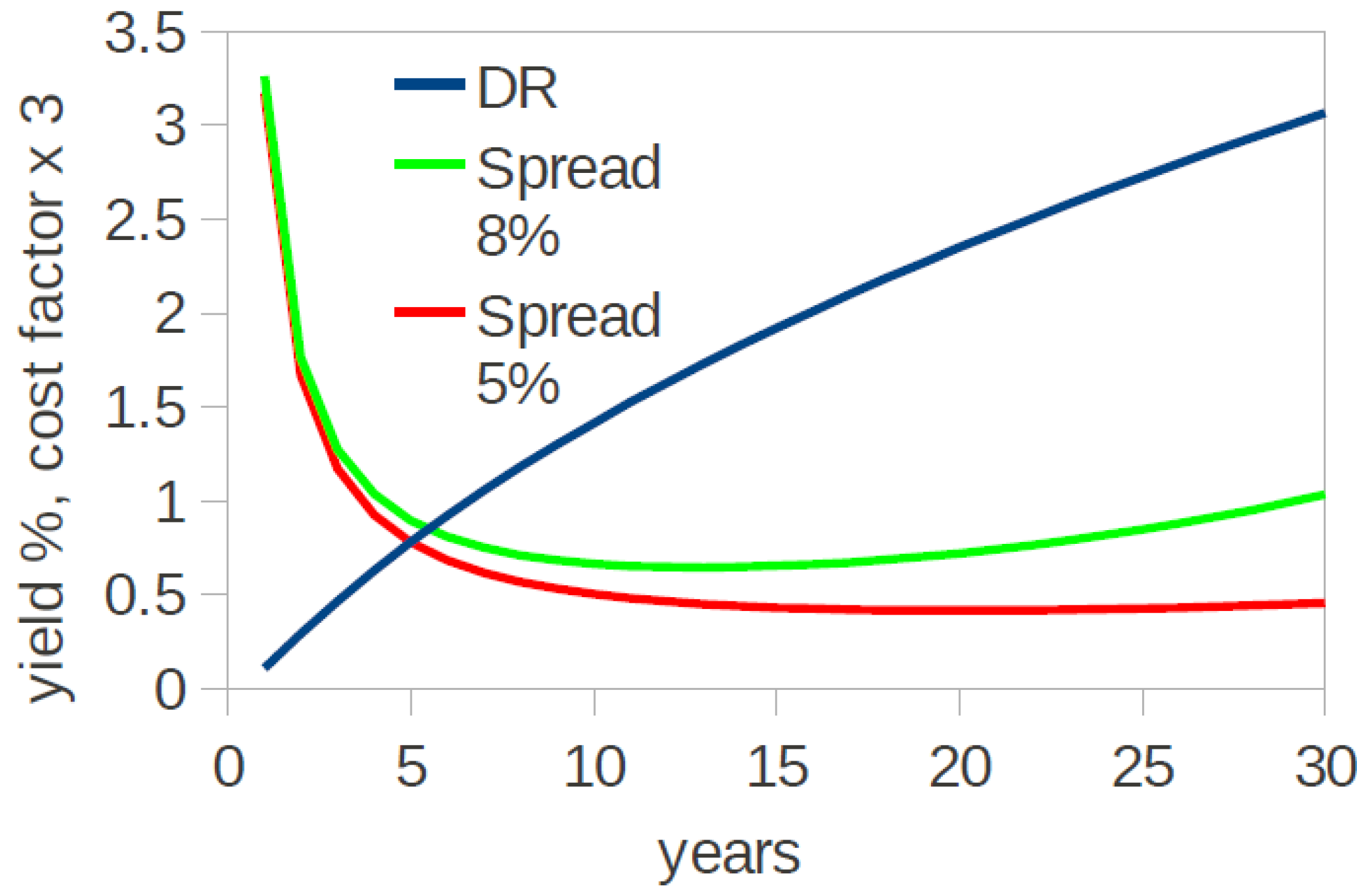
We now present an analysis of the dependence of the nominal LCOE on N, SDR, DR, and r based on Equation (5). First, we estimate the behavior of LCOE as a function of N and for SDR = 0.6% [13]. The increase of lifetime of OPV modules was identified in Ref. [2] as essential to the achievement of economic viability. The cost was found to drop with N and largely to level off after 15 years [2]. In our analysis, we used a model term structure of the US Treasury market shown in Figure 1 to obtain DR at any N (we neglect the small difference in yields between zero-coupon and conventional bonds which is unessential for the present analysis). The spread of r over DR was held fixed at 5% or 8% (for a maximum borrowing rate of about 11% at 30 years). In reality, the credit risk is term-dependent with the possibility of longer dated maturities having a wider or narrower spread over r₀. The assumption of fixed spread is for the generality of the argument, and it does not affect the conclusions.

The resulting dependence of the cost factor defined in Equation (6),

(6)

on N is also shown in Figure 1. The cost factor bottoms at N_min which depends on the credit spread and increases afterwards. The increase is faster for higher values of r. This is the true influence of the borrowing rate: it limits both the minimum cost and the optimal N due to escalating interest cost. In Fig. 7 of Ref. [2] (analogous to our Figure 1), the extent of the drop from N = 1 to N_min is slightly larger, and the cost keeps decreasing with N seemingly forever. Here, for simplicity and as in Ref. [6], we assumed that the duration of the loan is equal to the lifetime of the installation, which does not have to be the case.

Figure 1. A model US Treasury yield curve (blue) and the cost factor, Equation (6) for the spread over the risk-free rate of 5% (red) and 8% (green). A sample US Treasury yield curve was taken from www.finance.yahoo.com. The equation we used is yield, % = 0.0034 × (1.2892ln(years) + 2.7061)^3.473272, which approximates the yield curve as of October 3, 2011.

Figure 1. A model US Treasury yield curve (blue) and the cost factor, Equation (6) for the spread over the risk-free rate of 5% (red) and 8% (green). A sample US Treasury yield curve was taken from www.finance.yahoo.com. The equation we used is yield, % = 0.0034 × (1.2892ln(years) + 2.7061)^3.473272, which approximates the yield curve as of October 3, 2011.

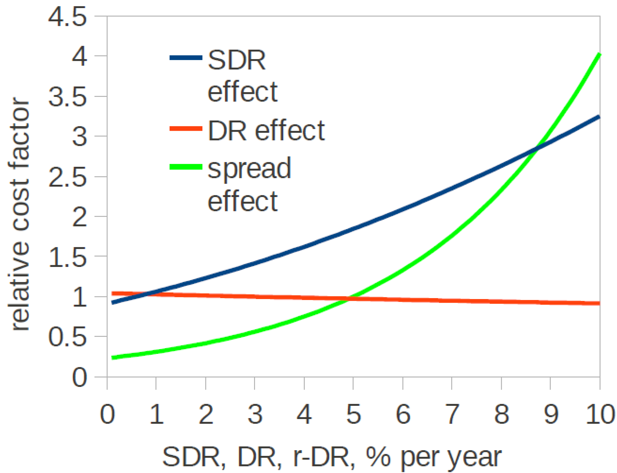
In Figure 2, we plot the relative cost factor for different SDR, for different DR at a fixed spread r-DR = 5%, and for different credit spreads at DR = 3%, for N = 30 years. The curves are normalized to the cost at r-DR = 5%, SDR = 0.6%, and DR = 3%. The system degradation rate has a rather mild effect on cost, doubling it as SDR increases from 0.6% to about 5.6% per year, where at the end of service the installation will have only about 18% of its initial output. An increase of DR has the effect of slightly decreasing the relative cost. This is because an increase of DR lowers the present cost of future obligations even as r grows as long as the credit risk (r-DR) does not increase. This DR = r₀ is determined by macroeconomic conditions and monetary policy and is not influenced by the borrower or by a particular industry. Both SDR and DR are less important than the conversion efficiency or insolation, which influence the relative cost per kWh as 1:1 (i.e., ).

Figure 2. The effect on cost of system degradation rate (blue), discount rate (red), and credit spread (green). The curves are normalized to the cost at r-DR = 5%, SDR = 0.6%, and DR = 3%.

Figure 2. The effect on cost of system degradation rate (blue), discount rate (red), and credit spread (green). The curves are normalized to the cost at r-DR = 5%, SDR = 0.6%, and DR = 3%.

The credit risk specific to the borrower has the most profound effect of all factors. The cost can be decreased four-fold for a near risk-free borrower, whereas it doubles if the spread is increased from 5% to 7.5%. Specifically, for low-risk borrowers (spreads below about 4%), the response of the cost to relative change in spread is smaller than to relative change in conversion efficiency and insolation. Research into improvement of solar-to-electricity conversion efficiency is thereby re-given the importance it lost in Ref. [6].

The models we considered do not provide a complete cost-benefit analysis. Cost-benefit models will have to include the cash flow from electricity sales [9]. That cash flow should be discounted using the risk-free rate plus premiums for the risks to fail to produce and to collect sales proceeds, which does not have to add up to the borrowing rate (e.g., due to different term structures or collaterization conditions for moneys owed by and to the company); using the latter could lead to an arbitrage opportunity whereby valuations will be depressed for riskier borrowers, and an entity with a better risk profile could buy the enterprise and enjoy higher valuations. Needless to say, the present argument about the appropriate discount rate is applicable to other industries as well [11].

4. Conclusions

In summary, we proposed a corrected description of financial factors influencing the cost of energy in the LCOE model, specifically solar energy, vs. recently proposed models [2,6,7]. Our model establishes the importance of the physical parameters, i.e., conversion efficiency (in contrast to Ref. [6]) and the need for a low credit risk of the enterprise (in contrast to both Ref. [2] and Ref. [6]). While it is true that in most cases the discount rates used by both governments and companies are not risk-free [7,14], we have shown rigorously that there is a problem (arbitrage opportunity) of using non-risk-free rates when comparing the cost of energy between different technologies and producers. We hope that the issues addressed in this Communication will help develop better quantitative models of economic performance of renewable energy installations and avoid mis-allocation of research effort and of capital.