What Should You Pay to Cap your ARM?—A Note on Capped Adjustable Rate Mortgages

Abstract

In this paper, an Adjustable Rate Mortgage (ARM) and a Fixed Rate Mortgage (FRM) are formalized and studied in a simple continuous-time setting under the assumption of a simple one-factor Affine Term Structure (ATS). Through an application of existing results from ATS theory, it is shown that when the short rate reaches a certain pre-determined boundary, the constant payment stream on a new FRM equals the payments on an existing ARM. Hereby, this paper provides a theoretical build-in cap on the formalized ARM. The finite boundary for the short-rate suggests that certain caps on ARMs should (in theory) be offered free of charge.

1. Introduction

In this paper, the relation between the payments on a formalized Adjustable Rate Mortgage (ARM) and a Fixed Rate Mortgage (FRM) is studied in a simple continuous-time setting under the assumption of a simple one-factor Affine Term Structure (ATS). The motivation for the study is to provide theoretical insights into the debate on the features of common loan products on the (Danish) mortgage market. It is shown that the payments on the formalized ARM equals the payments on a new FRM when the short rate hits a certain boundary. The boundary is a deterministic function in time, which can be determined at the initiation of the mortgage. In conclusion, the boundary provides a build-in cap on the adjustable rate of the formalized ARM. The conclusion relies on an assumption of a one-factor ATS, and is a direct consequence of existing results provided by Keller-Ressel and Steiner [1] regarding the yield curve shapes of ATSs. The two mortgage products are formalized following the work of Nordfang and Steffensen [2]. The simple theoretical setting combined with the formalization highlights defining features of the two products and enables a straightforward analysis of the theoretical relations between the two products. There exists a vast body of literature on interest rate models, but there is no consensus on a term structure model that sufficiently captures the real interest rate dynamics while remaining mathematically tractable (e.g., [3,4] and the references therein). The class of (conservative) ATSs primarily fulfil the latter, at the cost of realism. Over time, empirical studies have challenged the ATS model, but despite the critiques, many of the studies still acknowledge that some of the defining features of the ATSs do in fact mimic important aspects of the real interest rate. In the detailed study of Dahlquist [5], both the Cox–Ingersoll–Ross (CIR) model and Vasicek model are concluded to be good fits for the short rate behavior in several countries. The class of ATSs provides a well-explored theoretical foundation, and this study gives a practical interpretation of some of the theoretical results. In a numerical example, it is shown how the boundary at which the interest rate can be fixed is at a higher level than the initial FRM interest. This points out shortcomings of the usual budget assessment of ARM borrowers in the Danish mortgage market today.

The paper is organized as follows: in Section 2, we introduce a simple bond market with stochastic interest rate. In Section 3, we introduce the formalized ARM and FRM originally presented in [2]. In Section 4, we summarize the results from ATS theory provided by Keller-Ressel and Steiner [1]. The results are presented only in the special case of the simple interest rate model of Section 2. In Section 5, we present a novel implication of the ATS results in the model of Section 2: the discovery of a build-in cap on the formalized ARM presented in Section 3. In Section 6, we present a numerical example of the cap in the special case of a Vasicek modelled short rate (see [6]). In Section 7, we conclude on the findings.

2. The Market Model

Assume that there exists a (frictionless) market for Zero Coupon Bonds (ZCB) for every maturity $T>0$ and a risk-free asset—the money account—with dynamics

$$dB\left(t\right)=r\left(t\right)B\left(t\right)dt,B\left(0\right)=1,$$

for some stochastic short rate $r\left(t\right)$, specified as the solution to the stochastic differential equation

$$dr\left(t\right)=\mu (t,r\left(t\right))dt+\sigma (t,r\left(t\right))d{W}^Q\left(t\right).$$

(1)

Let $P^T\left(t\right)$ denote the price at time t of a ZCB with maturity T, and recall the martingale representation of the bond prices, defining

$$G(t,r,T):=E_{t,r}^Q\left[e^{-{\int }_t^{T}r\left(s\right)ds}\right],$$

such that the bond price can be written as

$$P^T\left(t\right)=G(t,r\left(t\right),T).$$

(2)

Let $A^T\left(t\right)$ denote the price at time t of an Annuity Bond (a constant payment stream of 1) with termination at time T. With this notation, the relation $A^T\left(t\right)={\int }_t^T{P}^s\left(t\right)ds$ is observed. Finally, let $q_r^T\left(t\right)$ denote the annuity factor at time t with maturity at time T and constant interest rate r:

$$q_r^T\left(t\right)={\int }_t^T{e}^{-{\int }_t^{s}rd\tau }ds=\frac{1}{r}(1-e^{-r(T-t)}).$$

(3)

If the term structure in the complete bond-market is assumed to be one of certain well-behaved types (e.g., Vasicek [6]), then the prices $P^T\left(t\right)$ and $A^T\left(t\right)$ can be determined in closed-form at any time t at the realization of the short rate $r\left(t\right)$. In the following, we will only consider the simple one-factor affine short rate model defined by

Definition 1

(A simple one-factor affine short rate). Assume that under the risk-neutral Q-measure, the short rate follows the dynamics in Equation (1) with μ and σ satisfying

$$\mu (t,r)=b+\beta r,$$

(4)

$$\frac{1}{2}{\sigma }^2(t,r)=a+\alpha r,$$

(5)

with $\beta \in \mathbb{R}$ and the remaining parameters satisfying either

$$\mathbf{1}\mathbf{)}a=0and\alpha ,b\in {\mathbb{R}}_{+}$$

$$\mathbf{2}\mathbf{)}a\in {\mathbb{R}}_{+},\alpha =0,andb\in \mathbb{R}.$$

Then the short rate is called a simple one-factor affine short rate.

3. Mortgage Products on the Danish Market

In this study, a mortgage product is defined as an agreement on a payment stream from a borrower to a lender. The payment stream can be deterministic or can consist of a set of rules agreed upon at the initiation of the loan. In a complete market with no arbitrage, the initially borrowed amount must equal the present value of the payment stream under the Q-measure. This equality can be enforced by a lump-sum payment at maturity, if necessary. In Denmark, mortgage products are commonly defined and communicated as an agreement on a certain interest rate profile through which the payment stream is uniquely determined by an annuity-factor with the agreed-upon interest. After agreeing on a certain interest rate profile, any specific loan described in this section is uniquely defined by the maturity T and the initial principal $H_0$ of the loan. The principal of the loan is the initially borrowed amount, and the outstanding principal is the amount after repayments to which the borrower pays interest (according to the chosen profile). The total payment stream on a loan include both interest and repayment of the loan (noting in particular the strict distinction between payment and repayment).

A simple theoretical setting is chosen to keep focus on the interest rate structure of the contracts, and thus several features that are common in the market (e.g., deferred repayments, prepayment of the mortgage, specific tax-rules, and transaction-costs on the loans) are not taken into account. The importance of these aspects is acknowledged, but the aspects are left for future research. In the following two subsections, the specification of the payment stream on a formalized FRM and ARM is stated. The formalization originates from [2], and we refer to that paper for a more detailed disposition.

3.1. Total Payments on the FRM

The constant total payment stream of a simple formalized FRM with initial principal $H_0$ at time $t=0$ and maturity T is determined by:

$$\overline{b}:=\frac{H_0}{A^T\left(0\right)}.$$

At any given time t, the market-value of a constant payment stream of one is exactly the price of an annuity-bond, and thus the market-value of the simple FRM is

$$\overline{M}\left(t\right):=\overline{b}{A}^T\left(t\right).$$

As a result, the constant total payment on the FRM can be written as

$$\overline{b}=\frac{\overline{M}\left(t\right)}{{\int }_t^T{P}^s\left(t\right)ds}.$$

It is noted that in this simple setting there is one unique fixed interest to pay on a fixed rate mortgage with a certain maturity. This is different to the reality of the (Danish) mortgage market, where the FRMs are callable at par and thus might have different (effective) interest rates for the same maturity (due to the influence of the market price of the call-option in the market). The unique interest is denoted $\overline{r}$, and it is determined as the solution to

$$A^T\left(0\right)={\int }_0^T{e}^{-\overline{r}(s-t)}ds.$$

3.2. Total Payments on the ARM

In the (Danish) mortgage market, the payments and principal on an ARM are determined by an annuity factor with the chosen adjusted interest rate profile. The payment stream on a formalized constantly adjusted ARM is thus at all times calculated as:

$$\widehat{b}\left(t\right)=\frac{\widehat{M}\left(t\right)}{{\int }_t^T{e}^{-r\left(t\right)(s-t)}ds},$$

(6)

where $\widehat{M}\left(t\right)$ denotes the market value of the ARM.

The market-value of an ARM equals the principal of the loan at every re-financing node. In the (theoretical) case of a constantly adjusted interest rate, the market value equals the principal at all times. Since the payments and principal are settled in an annuity manner, the (theoretical) constantly adjusted ARM in the Danish market can be considered as a negative position in the money account (see [2] for a detailed introduction to the Danish ARMs and the limit argument leading to this conclusion). In the case with initial principal $H_0$ and payment stream $\widehat{b}\left(t\right)$, the market value is thus specified by the dynamics

$$d\widehat{M}\left(t\right)=r\left(t\right)\widehat{M}\left(t\right)dt-\widehat{b}\left(t\right)dt$$

(7)

$$\widehat{M}\left(0\right)=H_0.$$

(8)

It is observed that the formalized ARM has a locally risk-free market value (and principal). However, the market value is—by construction—still stochastic. This is due to the payments defined by Equation (6), which are calculated by an annuity factor with the stochastic interest rate $r\left(t\right)$. We note that it is possible to define an ARM where the payment stream absorbs all of the uncertainty from the stochastic interest such that the principal and market value are entirely deterministic.

3.3. Relations between the FRM and the ARM

The FRM and the ARM introduced in this paper are in some respects each other’s opposite. The FRM has a deterministic and smooth (in fact, constant) payment stream, while the ARM has a stochastic and diffusive payment stream. On the other hand, the ARM has a smooth market-value throughout the duration of the loan, while the FRM has a diffusive market-value.

4. Results from Affine Term Structure Theory

In this section, the main result from [1] is stated. The theorems and definitions summarized here are presented in a version which only applies to the simple affine short rate model without jumps presented in Definition 1. When relevant, we refer to the corresponding original definitions and theorems from [1]. The original versions cover a general class of ATSs.

Proposition 1

(Proposition 3.4 in [1]). The short rate model of Definition 1 admits an ATS with the bond price specified through the function

$$G(t,r,T)=e^{A(T-t)+B(T-t)r},$$

(9)

where $A(·)$ and $B(·)$ are functions determined as the solutions to the system

$${\partial }_{x}A\left(x\right)=F\left(B\left(x\right)\right),A\left(0\right)=0,$$

$${\partial }_{x}B\left(x\right)=R\left(B\left(x\right)\right)-1,B\left(0\right)=0,$$

with

$$F\left(u\right):=a{u}^2+bu$$

(10)

$$R\left(u\right):=\alpha u^2+\beta u.$$

(11)

We refer to the proof of Proposition 3.4 in [1] for the case of a general regular ATS1.

It is immediately seen that the Vasicek and CIR models of the short rate are affine term structures in the sense of Definition 1, since they are specified by the Q-dynamics:

Vasicek:

$$dr\left(t\right)=(c_1-c_{2}r\left(t\right))dt+c_{3}d{W}^Q\left(t\right),(c_2>0)$$

CIR:

$$dr\left(t\right)=(c_1-c_{2}r\left(t\right))dt+c_3\sqrt{r\left(t\right)}d{W}^Q\left(t\right)$$

for some constants $c_1,c_2,c_3$.

Next, let the yield $Y\left(r\right(t),x)$ be defined as

$$Y(r\left(t\right),x):=-\frac{log{P}^{t+x}\left(t\right)}{x},$$

while remembering the suppressed short-rate dependence in the bond price as seen in Equation (2).

Definition 2

(Definition 3.8 in [1]). The yield curve $Y\left(r\right(t),x)$ is called

• Normal, if it is a strictly increasing function of x,
• Inverse, if it is a strictly decreasing function of x,
• Humped, if it has exactly one local maximum and no minimum on $(0,\infty )$

In addition, the yield curve is called Flat if it is constant over all $x\in \mathbb{R}$.

Finally, the main result from [1] is stated in the specific case of the simple short rate model.

Theorem 1

(Theorem 3.9 in [1]). Let the risk-neutral short rate process be specified by Definition 1. Then, the following hold:

• The yield curve $Y\left(r\right(t),·)$ can only be normal, inverse, or humped.
• Define

  $$r_{norm}:=\frac{-4a-b\beta +b\sqrt{{\beta }^2+4\alpha }}{4\alpha +{\beta }^2-\beta \sqrt{{\beta }^2+4\alpha }}$$

  (12)

  $$r_{inv}:=\left\{\begin{array}{cc}-\frac{b}{\beta }\hfill & if\beta <0\hfill \\ +\infty \hfill & if\beta \ge 0\hfill \end{array}\right.$$

  (13)

  The yield curve is normal if $r\left(t\right)\le r_{norm}$, humped if $r_{norm}<r\left(t\right)<r_{inv}$, and inverse if $r\left(t\right)\ge r_{inv}$.

We refer to the proof of Theorem 3.9 in [1] for the case of a general regular ATS2.

The result partly dates back to the original paper by Vasicek [6], where the above relations were provided for the Vasicek term structure. The result was later extended by Keller-Ressel and Steiner [1], who provided barriers for a more general class of ATSs.

To be clear about what this means, having the yield-curve of the ATS from Theorem 1 gives:

$$Y(r\left(t\right),x)=\frac{-A\left(x\right)-r\left(t\right)B\left(x\right)}{x},$$

and since—by definition—the yield at time zero always equals the short interest $Y\left(r\right(t),0)=r\left(t\right)$, then the boundaries above entail the following relations for all $x>0$:

$$\begin{array}{cc}\hfill 1)& Y(r\left(t\right),x)>r\left(t\right)\mathrm{when}r\left(t\right)\le r_{\mathrm{norm}}\hfill \end{array}$$

(14)

$$\begin{array}{cc}\hfill 2)& Y(r\left(t\right),x)<r\left(t\right)\mathrm{when}r\left(t\right)\ge r_{\mathrm{inv}}.\hfill \end{array}$$

(15)

From these boundaries and with the formalization of the mortgages from the previous sections, it is possible to analyze the effect on the payment stream when a borrower changes mortgage from an ARM to an FRM.

5. Implications to the Formalized Mortgage Products

5.1. Transition from ARM to FRM

First, it is assumed that the borrower who initially chooses an ARM is only interested in fixing this by switching to an FRM if this can be done continuously. By this, the borrower fixes the interest at the exact time when the total payment of the borrowers existing ARM equals that of a new FRM. In addition, it is assumed that the borrower only chooses an ARM initially when the initial total payments on the ARM are smaller than those of an FRM. The borrower who has initiated an ARM will at any time t have to refinance the market value $\widehat{M}\left(t\right)$, as specified in Equations (6) and (7). By definition, the constant total payment stream on a new FRM is thus at any given time t determined by:

$${\overline{b}}_{NEW}:=\frac{\widehat{M}\left(t\right)}{A^T\left(t\right)}.$$

Meanwhile, the total payments on the ARM, $\widehat{b}\left(t\right)$, are at all times calculated by Equation (6), and it is concluded that the following relation holds at all times t:

$${\overline{b}}_{NEW}=\widehat{b}\left(t\right)\frac{{\int }_t^T{e}^{-r\left(t\right)(s-t)}ds}{A^T\left(t\right)}.$$

From this, it is clear that the only times where the payment stream is continuous when making a transition from an ARM to an FRM is when

$${\int }_t^T{e}^{-r\left(t\right)(s-t)}ds=A^T\left(t\right).$$

Based on these considerations, the main result is now presented.

Theorem 2.

In a market model with short rate specified by Definition 1 with $\beta <0$, there exists an $r^{*}\left(t\right)$ for all $t\ge 0$ at which one can shift from the formalized ARM to a new FRM while maintaining a continuous payment stream. The boundary $r^{*}\left(t\right)$ can be determined at time 0 (numerically, if not analytically) as the solution to

$${\int }_t^T{e}^{A(s-t)+B(s-t)r^{*}\left(t\right)}ds={\int }_t^T{e}^{-r^{*}\left(t\right)(s-t)}ds,$$

and $r_{norm}\le r^{*}\left(t\right)\le r_{inv}$ for all $0<t<T$. The upper bound $r_{inv}$ and lower bound $r_{norm}$ are determined analytically as specified in Theorem 1.

Proof. 

As a result of the yield-curve regions in Theorem 1 and the resulting relations 1) and 2) in Equations (14) and (15), the following relations hold when assuming $t<T$:

$$r\left(t\right)\ge r_{\mathrm{inv}}\Rightarrow {\int }_t^T{e}^{A(s-t)+B(s-t)r\left(t\right)}ds>{\int }_t^T{e}^{-r\left(t\right)(s-t)}ds\Rightarrow {\overline{b}}^{NEW}\left(t\right)<\widehat{b}\left(t\right)$$

$$r\left(t\right)\le r_{\mathrm{norm}}\Rightarrow {\int }_t^T{e}^{A(s-t)+B(s-t)r\left(t\right)}ds<{\int }_t^T{e}^{-r\left(t\right)(s-t)}ds\Rightarrow {\overline{b}}^{NEW}\left(t\right)>\widehat{b}\left(t\right).$$

From these relations, and since the payment streams $\widehat{b}\left(t\right)$ and ${\overline{b}}^{NEW}\left(t\right)$ are continuous, it is concluded that for every t there exists at least one $r^{*}\left(t\right)\in [r_{\mathrm{norm}},r_{\mathrm{inv}}]$ for which ${\overline{b}}^{NEW}\left(t\right)=\widehat{b}\left(t\right)$. ☐

By this, a cap on the ARM is provided “free of charge”. It is concluded that if starting with an ARM, then this mortgage can be converted to an FRM while maintaining continuous payments if the short rate reaches $r^{*}\left(t\right)$. To sum up:

The interest on the ARM can be fixed with a continuous payment stream if $r\left(t\right)=r^{*}\left(t\right)$.

Since the boundary $r^{*}\left(t\right)$ is dependent on time, it might be hard to communicate to the customers.

It is furthermore possible to calculate a boundary for the payment stream throughout the duration of the mortgage. The short-rate has been smaller than the boundary $r^{*}\left(t\right)$ at all times, and it is therefore guaranteed that the principal is also smaller than a (hypothetical) annuity loan with the boundary-rate $r^{*}\left(t\right)$. So, at time zero, you have an upper boundary for the interest until you do the switch $r^{*}\left(t\right)$. This interest can be used to calculate an upper bound for the principal of the ARM at the time where you do the switch:

$$d\mathrm{Bound}\left(t\right)=r^{*}\left(t\right)\mathrm{Bound}\left(t\right)dt-b^{*}\left(t\right)dt,$$

$$\mathrm{Bound}\left(0\right)={\mathrm{Kap}}_0,$$

with (hypothetical) annuity payment stream $b^{*}\left(t\right)$ defined by

$$b^{*}\left(t\right):=\mathrm{Bound}\left(t\right)/q_{r^{*}\left(t\right)}^T\left(t\right),$$

recalling the annuity factor $q_r^T\left(t\right)$ defined in Equation (3). In conclusion,

$$\mathrm{Bound}\left(t\right)={\mathrm{Kap}}_{0}exp\left\{{\int }_0^t-\frac{r^{*}\left(s\right)e^{-r^{*}\left(s\right)(T-s)}}{1-e^{-r^{*}\left(s\right)(T-s)}}ds\right\}.$$

So, at any given time $t>0$, providing the short rate has been smaller than $r^{*}\left(s\right)$ for all $0\le s<t$, it is guaranteed that:

$$\widehat{M}\left(t\right)<\mathrm{Bound}\left(t\right),$$

and through this, it is ensured that

$${\overline{b}}^{NEW}\left(t\right)<b^{*}\left(t\right).$$

6. Numerical Example with Vasicek Short Rate

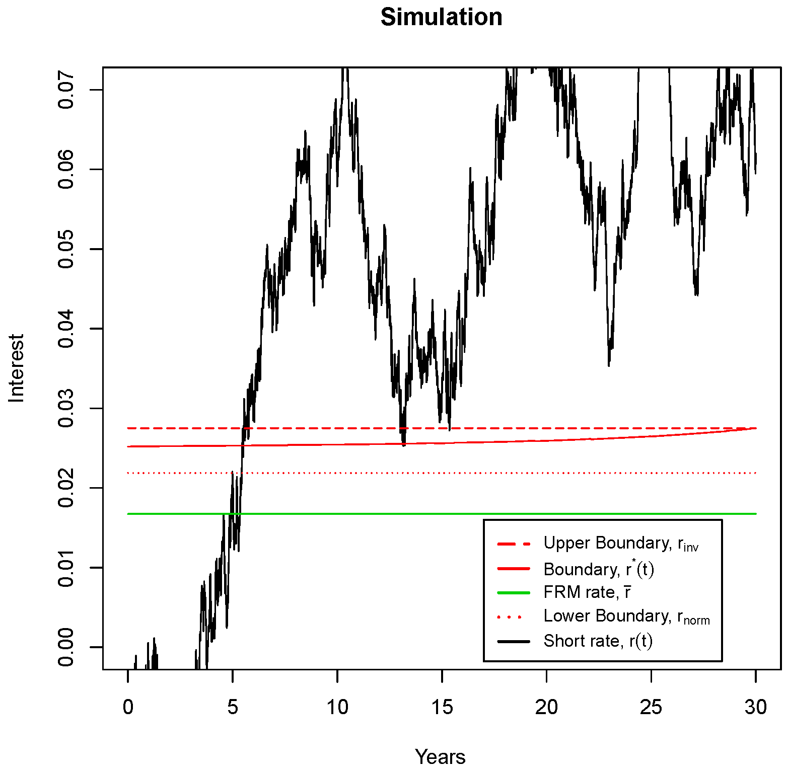
In a Vasicek setting, the above results are particularly simple. Assuming short-rate P-dynamics:

$$dr\left(t\right)=\kappa (r_v-r\left(t\right))dt-{\sigma }_{v}d{W}^P\left(t\right),$$

and assuming a constant market price of risk, λ, then the Q-dynamics are,

$$dr\left(t\right)=\kappa (r_v+{\sigma }_v\lambda /\kappa -r\left(t\right))dt-{\sigma }_{v}d{W}^Q\left(t\right).$$

The F- and R-function defined in Equations (10) and (11) are identified as

$$F\left(x\right)=\kappa (r_v+{\sigma }_v\lambda /\kappa )x+\frac{1}{2}{\sigma }_v^2{x}^2$$

$$R\left(x\right)=-\kappa x.$$

As a result, it is possible to determine the boundary $r^{*}\left(t\right)$ numerically. Furthermore, the upper and lower bounds are given by Keller-Ressel and Steiner [1], referred in Equations (12) and (13) of Theorem 1 above:

$$r_{\mathrm{inv}}=r_v+{\sigma }_v\lambda /\kappa$$

(16)

$$r_{\mathrm{norm}}=r_v+{\sigma }_v\lambda /\kappa -{\sigma }_v^2/{\kappa }^2.$$

(17)

6.1. Simulation

The numerically calculated boundary $r^{*}\left(t\right)$ and the upper and lower bound $r_{\mathrm{inv}}$ and $r_{\mathrm{norm}}$ can be viewed in a numerical example with a short rate simulation in Figure 1. The parameters used for the Vasicek short rate model in the example are the same as used by Kraft and Munk [7], and can be viewed in

Table 1. Parameters for the baseline example.

Parameter	Variable	Value
Maturity	T	30
Mean reversion rate	κ	0.2
Long-term short rate	$r_v$	0.02
Short rate volatility	${\sigma }_v$	0.015
Sharpe ratio of bond	λ	0.1
Initial short rate	$r_0$	–0.0034

. The initial interest for the simulation path is set at $r_0=-0.0034$, reflecting the 1-week Copenhagen Interbank Offered Rate (CIBOR) of 22 December 2016. A simple calculation of the prices of the Danish Government Bonds has been made under the assumption of the short rate model (while assuming zero credit risk), and these prices are compared to the market closing prices in

Table 2. Comparison of the prices of Danish Government Bonds in the model and in reality, as of 22 December 2016.

Bond	Model Price	Closing Price
4.0%, 15 November 2017	103.96	104.17
4.5%, 15 November 2039	150.31	171.92
7.0%, 10 November 2024	141.03	153.77

. As expected, it is not possible to replicate the closing prices, but we see that the model parameters (very) roughly capture the current price level in the Danish bond market.

The example shows that the borrower with the ARM can fix the interest-rate just before year five. The boundary at which the interest rate can be fixed is calculated at the initiation of the loan, and it can be communicated to the borrower at the initiation of the loan at which level the interest can be fixed. However, it is observed that the interest is fixed at a higher level than the initial FRM interest. This is in contrast to common financial advice in the Danish mortgage market, where customers are usually assessed on their ability to take on the risk of an ARM by securing that they have room in their budget for the payments on an (immediately initiated) FRM.

With the particular parameters used in this example, the upper bound for the boundary $r^{*}\left(t\right)$ is $r_{\mathrm{inv}}=0.0275$. As such, the customer who initiates an ARM with the current short rate $r_0=-0.0034$ is guaranteed a cap on the mortgage rate of less than $2.75\%$, offered free of charge. This is in contrast to the level and price of caps found in the market today. As an example, the Danish mortgage lender Nykredit offers a cap on their ARM at a level of 4%. The cap only applies for the next 10 years, at which state a new cap is determined, and the cap is offered at a price of 0.55% in addition to the short rate throughout the duration of the cap. Although the products are not entirely comparable to the simple setting of this paper, it suggests that the market prices for caps on ARMs are high. It is also noted that many Danish mortgage brokers no longer offer caps on ARMs, as there is very little demand.

In addition, it is observed that the rate on the FRM initiated immediately at time $t=0$ is $\overline{r}=0.0167$. When a household is allowed by a mortgage lender to take out an ARM in Denmark today, the common practice is to check if the household has enough room in their budget today for mortgage payments corresponding to the FRM rate, $\overline{r}$. However, when the ARM is chosen and the short rate increases, then the level at which the household can fix the rate on their mortgage (continuously) is significantly above $2\%$ (with a lower bound $r_{\mathrm{norm}}=0.0219$ and upper bound of $r_{\mathrm{inv}}=0.0275$). One can thus argue that the budget-test which mortgage lenders use to assess the economy of a household should be carried out in terms of the conservative upper bound $r_{\mathrm{inv}}=0.0275$ determined in this study. This would give a more appropriate benchmark for the budget-risk involved when choosing an ARM.

6.2. Sensitivity

The sensitivity of the boundary $r^{*}\left(t\right)$ is studied in terms of the upper and lower bounds $r_{\mathrm{inv}}$ and $r_{\mathrm{norm}}$. In Equations (16) and (17), it is seen that the level of $r^{*}\left(t\right)$ is driven by the level of the long-term short rate $r_v$ with the addition of the term ${\sigma }_v\lambda /\kappa$. Increasing the short rate volatility produces a higher level for the transition rate $r^{*}\left(t\right)$, as the FRM price increases faster with high volatility. Likewise, a high market price on risk results in a high level of $r^{*}\left(t\right)$. In contrast, when the mean reversion rate κ is high, the upper bound $r_{\mathrm{inv}}$ will be closer to the long-term rate $r_v$, since the short rate will quickly adjust to the long-term level, and thus the price of the FRM will not be as sensitive to the level of the current short rate.

7. Conclusion

This study has demonstrated practical consequences of an ATS assumption in a simplified version of the Danish mortgage market. In particular, this study provides a theoretical upper boundary for a smooth transition from a formalized ARM offered in the Danish market to a new FRM. By this, the study provides a theoretical cap on the ARM free of charge. This discovery highlights that the choice of an ARM does not equal an acceptance of risking exorbitantly high payments. In addition, the boundary provides a level which can be presented to future loan takers in the choice between an ARM and an FRM. Finally, the practical consequences of the theoretical assumptions encourage further research to back-test the theoretical results on the Danish mortgage market.

References

1. M. Keller-Ressel, and T. Steiner. “Yield curve shapes and the asymptotic short rate distribution in affine one-factor models.” Financ. Stoch. 12 (2008): 149–172. [Google Scholar] [CrossRef]
2. M.B. Nordfang, and M. Steffensen. “Portfolio Optimization and Mortgage Choice.” J. Risk Financ. Manage. 10 (2017): 1. [Google Scholar] [CrossRef]
3. Q. Dai, and K. Singleton. “Term Structure Dynamics in Theory and Reality.” Rev. Financ. Stud. 16 (2003): 631–678. [Google Scholar] [CrossRef]
4. A. Episcopos. “Further evidence on alternative continuous time models of the short-term interest rate.” J. Int. Financ. Mark. Inst. Money 10 (2000): 199–212. [Google Scholar] [CrossRef]
5. M. Dahlquist. “On alternative interest rate processes.” J. Bank. Financ. 20 (1996): 1093–1119. [Google Scholar] [CrossRef]
6. O. Vasicek. “An equilibrium characterization of the term structure.” J. Financ. Econ. 5 (1977): 177–188. [Google Scholar] [CrossRef]
7. H. Kraft, and C. Munk. “Optimal housing, consumption, and investment decisions over the life cycle.” Manage. Sci. 57 (2011): 1025–1041. [Google Scholar] [CrossRef]
Figure 1. Simulation of the short-rate under the Vasicek assumption. FRM: Fixed Rate Mortgage.
Ijfs 05 00010 g001