
A Dynamic Programming Approach for Pricing Weather Derivatives under Issuer Default Risk

1
Ladislaus von Bortkiewicz Chair of Statistics, School of Business and Economics, Humboldt-Universität zu Berlin, Unter den Linden 6, 10099 Berlin, Germany
2
Sim Kee Boon Institute for Financial Economics, Singapore Management University, 90 Stamford Road, 6th Level, School of Economics, Singapore 178903, Singapore
*
Author to whom correspondence should be addressed.
†
Current address: Ladislaus von Bortkiewicz Chair of Statistics, School of Business and Economics, Humboldt-Universität zu Berlin, Unter den Linden 6, 10099 Berlin, Germany.
‡
These authors contributed equally to this work.
Int. J. Financial Stud. 2017, 5(4), 23; https://doi.org/10.3390/ijfs5040023
Submission received: 16 September 2017
/
Revised: 15 October 2017
/
Accepted: 16 October 2017
/
Published: 20 October 2017
(This article belongs to the Special Issue Recent Developments in Numerical Methods for Option Pricing)
Abstract
:Weather derivatives are contingent claims with payoff based on a pre-specified weather index. Firms exposed to weather risk can transfer it to financial markets via weather derivatives. We develop a utility-based model for pricing baskets of weather derivatives under default risk on the issuer side in over-the-counter markets. In our model, agents maximise the expected utility of their terminal wealth, while they dynamically rebalance their weather portfolios over a finite investment horizon. Using dynamic programming approach, we obtain semi-closed forms for the equilibrium prices of weather derivatives and for the optimal strategies of the agents. We give an example on how to price rainfall derivatives on selected stations in China in the universe of a financial investor and a weather exposed crop insurer.
1. Introduction
Weather derivatives (WDs) are contingent claims with payoffs determined by future weather events as temperature, snowfall, and rainfall. Hedging with WDs reduces exposure to weather volatility and stabilises profits of a weather exposed agent. Firms operating in energy, tourism, agriculture, and insurance sectors use WDs to hedge their weather risks. Investigations in Peréz-González and Yun (2013) show that weather risk management with WDs leads to an increase in firm value. Moreover, WDs are also attractive for a purely financial investor as their payoffs are acyclic, uncorrelated with financial assets, and, therefore, contribute to portfolio diversification.
Frequently, the structure of agent’s weather exposure is complicated, such that, it is more beneficial to purchase a basket of WDs on several underlying weather indices rather than on a single one to manage weather risks in an optimal way. For a financial investor, positions in multiple WDs strengthen the positive portfolio diversification effect. To increase the hedging efficiency and to achieve a higher degree of portfolio diversification, both weather exposed business and financial investors are, therefore, interested in holding a portfolio of multiple WDs. While valuing baskets of such derivatives, market participants should also account for the dependence in the underlying weather indices.
We develop a simple utility-based model for pricing such baskets of customised WDs on multiple dependent underlying indices. We address here the problem of WD pricing in over-the-counter (OTC) markets, where fewer interested agents transfer their specific non-financial weather risks among themselves through creating and trading customised weather dependent claims. We perceive a model which is flexible enough to handle a wide range of customised WDs and allows dynamic trading in the sence that the agents rebalance their portfolios (or renegotiate the contracts) at some predetermined discrete time points in their finite investment horizon. As in Çanakoǧlu and Özekici (2009) we use a dynamic programming approach for portfolio optimisation combined in our case with zero-net-supply condition for WDs to determine their equilibrium prices.
We choose an equilibrium pricing approach based on utility maximisation for several reasons. First, we anticipate that the OTC transactions of WDs involve a limited number of participants. Thus, the interaction of their individual supply and demand functions will give the equilibrium price. Further, due to the market incompleteness standard arguments imposing an existence of a unique pricing measure fail, see Heath et al. (1992). Models based on pure weather dynamics impose restrictive assumptions in order to choose the appropriate equivalent martingale measure, see Alaton et al. (2002), Benth et al. (2007), and López Cabrera et al. (2013). In our model, involved agents construct WD securities in zero net supply, thus, they complete the WD market. Moreover, the chosen utility-based pricing approach naturally reflects the risk attitudes of each agent and facilitates via dynamic programming the derivation of explicit prices for WDs in a multi-period framework.
Most previous works on utility-based WD pricing either fail to price derivatives on multiple dependent underlying indices simultaneously (Carmona and Diko 2005; Lee and Oren 2010; Leobacher and Ngare 2011) or they impose restrictive assumptions on the dynamics of the underlying weather indices (Horst and Müller 2007; Chaumont et al. 2006). Consumption based model of Cao and Wei (2004) prices multiple WDs in an extended pure exchange economy of Lucas (1978) on the macroeconomic level and is not feasible for a limited number of weather market participants and a short contract duration typical for OTC markets. We contribute to this literature by providing a model for pricing baskets of customised WDs on multiple dependent underlying indices. In our framework, market participants account for the possible dependence between the weather indexes that determine the payoffs of their weather portfolios. The applicability of our pricing model is not restricted to any particular type of WDs. Various kinds of WDs can be priced in our framework.
Our further contribution is the introduction of counterparty default risk into the pricing model for WDs. The importance of counterparty default risk for pricing was addressed, for example, in Hull and White (1995), Jarrow and Turnbull (1995), and Wu and Chung (2010). We show that the introduction of a non-zero issuer default probability significantly depresses the demand for WDs through correcting expectations of future portfolio payoffs in utility terms downwards.
We illustrate our approach on pricing rainfall derivatives. These derivatives can be used to hedge agricultural volumetric risks, see Musshoff et al. (2010). Traditionally, volumetric risk hedging in agriculture is taken over by the crop insurance as Glauber et al. (2002). Therefore, a crop insurer frequently faces indirect losses caused by rainfall surplus/deficit through its impact on crop production. Whenever the weather exposed income of such an insurer depends on rainfall outcomes in a number of geographical sites where the insured farmers are operating, a basket of rainfall derivatives should be used for hedging the risks.
We give the pricing example for China. Chinese farmers are exposed to pronounced weather risks as Turvey and Kong (2010). According to The World Bank (2007) the existing agricultural insurance schemes are too expensive for Chinese agricultural producers. Trading WDs can play an important role in transferring a part of the weather exposure of crop insurer to financial markets and so make crop insurance affordable for Chinese farmers.
Our empirical analysis addresses the effects of the increasing investment horizon, default risk, market volatility, and capital costs on the demand and on the supply for WDs.
The structure of the paper is as follows. In Section 2 we, first, derive the multi-asset dynamic pricing model for WDs in the absence of any default risk. Next, we extend the model to account for counterparty default risk and a possibility of an alternative financial investment. Section 3 shows an example of pricing rainfall derivatives using historical rainfall data for China and features a discussion of further applications. In Section 4 we summarise our results.
2. Dynamic Pricing Model for Weather Derivatives
In this section, we construct a dynamic pricing model for WDs with multiple assets. First, we introduce a market design and notation. Then, we derive equilibrium prices for WDs without any default risk. Next, we study the implications of counterparty default risk and of an alternative financial investment.
2.1. Assumptions and Notation
- Assets. There are WDs on S weather indices (at different geographical sites and/or on different weather events) that are priced at times At T the payoff of each WD is determined and the cash settlement takes place. The non-negative price of the WD on underlying s in time t is denoted as where and . The final value corresponds to the non-negative payoff of the sth WD. We denote the vector of prices at t as . Besides the WDs, a risk free asset with a constant per period return r is available. Trading with is not restricted in any way, that is, unlimited borrowing and lending at the interest r in each t is allowed. We assume there is no transaction costs on the asset market. No capital addition or withdrawals are possible throughout the investment horizon, such that the agents are exposed to self-financing constraints.
- Agents. There are heterogeneous market participants, indexed by i, with the risk preferences described by the exponential utility function of the form , where is the risk aversion of agent i. All agents have the same multi-period investment horizon of length T. They invest at and they consume their terminal wealth at . At agents rebalance their weather portfolios and renegotiate the prices for WDs. All agents are endowed with an initial wealth of zero monetary units. We distinguish between J buyers, indicated by subscript j, , who hedge weather exposure of their random income , and a purely financial investor, indicated by subscript m, who issues WDs. Each buyer holds a basket of WDs on the relevant weather indices to hedge weather caused fluctuations in her profits. The issuer holds positions in all S WDs. A portfolio of agent i includes shares of the corresponding WDs and shares of the asset . Both and are real valued, that is, all assets are perfectly divisible and short sales are allowed. We denote the value of ith agent’s portfolio at time t as , where . In each period t of the investment horizon, the agents maximise their expected utility of the terminal wealth with the available WDs and attain their demand and supply for the WDs. That is, in each period every agent i determines her self-financing trading strategy , in particular, she constructs the optimal hedging portfolio given the state of the system at time t. Partial market clearing with respect to WDs determines the equilibrium prices for the WDs.
- State. The observable state of the system at time t, denoted by , contains values of the underlying weather indices at t and the variables regarding default risk at t. The random state is characterised by the conditional distribution function . We assume that this transition function satisfies the Feller property Stokey et al. (1989). Expectation taken with respect to is denoted by .Each agent is faced with the following discrete time stochastic control system:where incorporates portfolio value of agent j with . are controls of the agent in the system (1). The law of motion maps to the next state of the stochastic system.
2.2. Pricing WDs without Default Risk
We now derive a dynamic pricing model for WDs with multiple assets under the market design described by assumptions 1 to 3. For the moment, we assume that there is no default risk. The terminal wealth of buyer j at T is her profit :
with being a random income that depends on some weather indices entering the final payoff . and are the payoffs of the risk free asset and of the basket of the WDs; together they constitute , the terminal portfolio value of buyer j. Let denote trading strategies of agent j from to T. Portfolio choice problem of buyer j in each is:
That is, in each period of the investment horizon T buyer j maximises expected utility of her terminal wealth with respect to all future trading strategies, subject to a self-financing portfolio.
The terminal wealth of investor m at T is:
with and being the payoffs of the WDs portfolio and the risk free asset respectively. Investor’s portfolio choice problem in each is:
In investor m maximises expected utility of her terminal wealth with respect to all future trading strategies, subject to a self-financing portfolio.
Note, that under assumptions 1 to 3, the constraints in the optimization problems (3) and (5) are non-empty, compact and continuous in and , is continuous and bounded, and transition function is Feller (by assumption). Thus, continuous law of motion ensures the existence of optimal solutions to the problems above and continuity of the value function (see Stokey et al. 1989, p. 62).
Following Pennacchi (2008) we solve the multi-period portfolio choice problems (3) and (5) using dynamic programming. Let denote the expected utility of agent i in time t. It depends on the agent’s current portfolio value , the current state , and the trading strategies in the time span to T (here indicated by subscript ). Let be the expected utility maximised with respect to the strategies of agent i from on. Formally, in each t is obtained by:
According to the principle of dynamic programming the expected utility of agent i in t can be rewritten as:
Combining (6) and (7), we obtain a recursive expression for :
with the boundary condition at T
and with .
Starting with and using (8), we recursively solve for supply and demand in each t for all the WDs, denoted in vector form as:
Imposing partial market clearing for WD securities (zero net supply), , delivers the equilibrium prices for all , where identifies the optimal values. Specific forms of buyer’s demand and investor’s supply are given in Propositions 1 and 2 below.
Proposition 1.
Let the utility function of the buyer j be of the exponential form with risk aversion . Let the assumptions 1 to 3 hold and let in (13) hold for . Then, jth buyer’s reverse demand for WD s, , and her optimal utility level are given recursively by:
for , and .
Proof.
See Appendix A. ☐
Proposition 2.
Let the utility function of the investor be of the exponential form with risk aversion . Let the assumptions 1 to 3 hold and let in (16) hold for . Then, investor’s reverse supply for WD s, , and her optimal utility level are given recursively by:
for , and .
Proof.
The proof is very similar to the proof of Proposition 1 and is omitted. ☐
The results above show that the reverse demand and supply for the sth WD at time t are determined by the interaction of the terms proportional to the marginal expected utility of the next period as well as future expected utilities in that embrace optimal future trading behaviour, . Moreover, the reverse demand and supply are both influenced by capital costs or risk-free rate r. Changes in r will, therefore, influence the resulting WD prices.
2.3. Default Risk
As we already mentioned, OTC derivatives are subject to counterparty default risk or credit risk as termed in Golden et al. (2007). In this section we consider incorporation of issuer default risk into the pricing model for WDs.
As in Golden et al. (2007), we consider dichotomous default risk modelled by a payoff proportion parameter with values in . While means that the counterparty fully meets its obligations in t, inherits the situation where the counterparty does not perform at all. We assume that is independent of all other random variables in the model, and , , where is the probability of investor’s default at . Parameters and are known to the buyers by t. Once the investor defaults, she is not going to meet any obligations in subsequent periods, and .
Clearly, under investor’s default risk, the payoff vector of the WDs is a multiple of , that is, . If the investor has met all her obligations up to period , then the contribution of the next period WD prices is . Hence, the jth buyer’s demand for WD s in (11) has to be modified to account for the default risk in the following way:
with
and .
To derive (17) we consider all probable outcomes of at each t. Thus, in , if we solve the maximisation problem (3) with the payoff of the WDs scaled by and equal to . As a result, we find , , and which is equal to:
with
If , , and
where .
We move one period backwards to . If now we maximise:
Note, that the expectation in the first line of (22) is taken under the joint distribution of and the other random variables of the model, and in the second line—only with respect to the joint distribution of the later ones. is in this case:
with
If then , , and
where . Then, the following expectation reads:
with
From (17) we observe that a non-zero issuer default probability influences adversely the demand for the WDs through correcting the expectations of the future portfolio values and the marginal expected utility of the WD payoffs downwards.
2.4. Alternative Investment
Frequently, the model assumptions implying that the agents’ portfolios contain only the risk free asset besides WDs do not hold. This will often be the case for the investor’s portfolio. In the following, we relax this restriction and allow the investor to invest in the financial market.
Let’s amend the assumptions made in Section 2.1 with the following:
- 1a
- Assets. Let assumption 1. hold. Let be a quoted price of an exchange traded financial asset at time t. While is given, is random, bounded, and predictable at t. Trading with is not restricted in any way, that is, short and long positions in the asset in each t are possible. We assume there is no transaction costs on the asset market. As before, no capital addition or withdrawals are possible throughout the investment horizon, such that the agents are exposed to self-financing constraints.
For example, can be a share value of an exchange traded fund tracking some financial portfolio, or it can represent the value of the market portfolio itself at t.
- 2a
- Agents. Let assumption 2. hold. Now, issuer m holds additionally shares of the exchange traded financial asset with exogenous price . Also, is real valued, that is, all assets are perfectly divisible and short sales are allowed. The value of the issuer’s portfolio at time t becomes .
As before, in each period t of the investment horizon, agents maximise their expected utility of the terminal wealth with the available WDs and attain their demand and supply for the WDs. That is, in each period issuer m determines her self-financing trading strategy , in particular, she constructs the optimal hedging portfolio given the state of the system at time t. Partial market clearing with respect to WDs determines the equilibrium prices for the WDs.
- 3a
- State. Let assumption 3. hold. The observable state of the system at time t, denoted by , contains additionally the quoted price . The random state is characterised by the conditional distribution function . Expectation taken with respect to is denoted by .
Under assumptions 1a-3a, the terminal wealth of investor m at T is:
with , , and being the payoffs of the WDs portfolio, the alternative financial investment, and the risk free asset respectively. Investor’s portfolio choice problem in each is:
As before, in each investor m maximises expected utility of her terminal wealth with respect to all future trading strategies, subject to a self-financing portfolio. The expected utility of the investor in t, , is now also a function of her trading strategies on the financial market, denoted as .
Keeping in mind these modifications and following the steps of Section 2.2, we have to modify investor’s supply for WD s in (14) in the following way:
for , and . In (33), should be chosen such that it satisfies:
Note, that now the reverse supply for the sth WD also depends on the position in the alternative financial investment. Thus, any changes in its price process will influence investor’s supply for the sth WD.
3. Pricing Weather Derivatives Using Weather Data
In this section, we show an example on how to price rainfall derivatives using historical weather data from China and discuss other applications of the pricing approach presented.
3.1. Pricing Chinese Rain
Chinese farmers are exposed to pronounced weather risks as Turvey and Kong (2010). According to The World Bank (2007) the existing agricultural insurance schemes are too expensive for Chinese agricultural producers. One of the causes might be the fact that crop insurer are exposed to variability in precipitation due to the impact of the later on farmers’ crop production. Trading WDs can play an important role in transferring part of the weather exposure to financial markets and so make crop insurance affordable for farmers. Since the weather exposed income of such a crop insurer is generally dependent on the rainfall in a number of geographical sites where the insured farmers are located, a basket of rainfall derivatives on the relevant sites should be used for hedging the risks. Motivated by this example, we illustrate pricing a basket of rainfall options on two weather stations Changde and Enshi1 located in an agricultural area of China.
3.1.1. Setup
Our representative buyer is an insurer who offers crop insurance to farmers in the agricultural area of Changde and Enshi is, therefore, exposed to fluctuations in the local rainfall amount. The company discovers that its income is highly dependent on the cumulative precipitation in Changde and Enshi during May, and wants to hedge its rainfall exposure by holding a portfolio of put options on cumulative rainfall in these sites. Suppose, there is an investor who wants to issue such rainfall derivatives on the two of the relevant sites: Changde and Enshi. Then, the parties consider pricing a basket of derivatives containing two put options on cumulative precipitation over May in Changde and Enshi. They construct the put options as plain vanilla options on the underlying rainfall indices computed as the sums of monthly rainfall over May measured in each of the sites. Both options mature at the end of the measurement period, that is, on the 31st of May. We also suppose that the parties agree to renegotiate the put prices in the middle of the measurement period: on the 15th of May.
Let denote the rainfall measured in the station i in day z. The cumulative precipitation over a period Z is then . Thus, a put option on the cumulative precipitation in Z in station i with strike (in precipitation units) has the payoff:
where k specifies the tick value of the option in monetary units.
Suppose, the insurer’s income exhibits a non-linear dependence to the rainfall index in May of the form with and parametrize the dependence of to the rainfall of Changde (indexed by 1) and Enshi (indexed by 2) respectively. Further parameters to specify are: the risk aversion , the strikes and the tick value monetary units per mm precipitation measured.
The log-return on the alternative investment in the investor’s portfolio is assumed to follow a normal distribution with zero mean and annual volatility in the law volatility scenario and in the high volatility scenario. The value of the alternative investment in is normalized to a hundred monetary units, that is .
We compute the prices for the put options assuming different investment horizons T. If , in (prior to the 1st of May) the agents negotiate the prices for the specified options under their current states of the world and respectively, and at (here, on 31 May) the settlement occurs according to the terminal time with realized payoffs . means that the agents additionally renegotiate the prices at (here, on 15 May). The renegotiation at takes place under the new circumstances arising from their new states and respectively. The final payments are then settled according to the realizations of . In our example, the state , includes the evolution of the rainfall, the observed price process , , , , and r. The evolution to the next state conditional on the realization of is described by continuous function . The terminal state of the insurer contains also her realised income .
3.1.2. Generation of Dependent Rainfall Paths on a Daily Basis
We use a model for multi-site rainfall generation proposed by Wilks (1998). This model accounts for spatial correlation of rainfall occurrences and rainfall amounts, and is flexible enough to describe different rainfall-based indexes. Based on Wilks (1998) we give the basic ideas of the model below:
Precipitation at time t in station is modelled as:
where takes values and represents a rainfall occurrence at time t in station and is a positive random variable for the rainfall amount. This structure ensures that equals zero whenever is zero and there is no rain and equals whenever rainfall occurs. are assumed to form a Markov chain with two states, wet and dry:
We take a first order Markov model where the probability of a wet day depends only on the state in the previous day. Our justification of this choice is based on the Bayesian information criteria (BIC), see Katz (1981) where the lowest value of the test statistics indicates the appropriate order of the Markov chain. The transition probabilities to the wet state are:
The multi-site feature is added to the model through the generation of correlated occurrences in neighbour locations. We define the threshold probability :
and can be generated using
Here is the cumulative distribution function of the standard normal distribution, , with such that the empirical correlations of the rainfall occurrences are mimicked in the generated rainfall occurrence series, see Wilks (1998) for further details.
The multi-site rainfall amount, conditioned on a rainy day, follows a mixture of two exponential distributions with a time dependent mixing parameter and time changing means . Following Wilks (1998) we can generate rainfall amounts at time t in site s using
where
and are normal covariates correlated such that the generated rainfall time series mimic the empirical correlation in the rainfall data.
Now we estimate the parameters for the multi-site rainfall generation in Changde and Enshi based on the rainfall data. Table 1 summarises the daily rainfall data for Changde and Enshi acquired via Research Data Centre of CRC 649 (Collaborative Research Centre 649: Economic risk).
BIC in Table 2 indicates that the first order Markov chain is appropriate to model the rainfall occurencies in the data.
The parameters for the rainfall amounts were estimated using maximum likelihood. For the analysed rainfall data and whereas and where the indices 1 and 2 refer to Changde and Enshi respectively. The empirical counterpart of appears to be 0.53, in order to mimic this correlation must be set to 0.76. The empirical counterpart of is 0.16 for the considered data, and in order to obtain this correlation in the generated rainfall series must be 0.25.
The results on fitting the mixture of two exponential distributions to , are presented in Table 3.
In our Monte Carlo example, we generate the correlated rainfall time series in Changde and Enshi using the estimated parameters and (36) times.
3.1.3. Results
By altering T, p, r and we obtain the put prices on the rainfall in Changde and Enshi under different market scenarios, see Table 4. All prices are normalized to the price obtained for , , and to enable the comparison.
The shift of the demand curve by changing probability to default and capital costs is shown in Figure 1.
The prices are significantly lower under a non-zero default probability and increasing capital costs. Whereas non-zero default probability has no effect on the supply of the WDs, the demand curve shifts downwards which results in lower equilibrium prices for the rainfall options. A higher risk-free rate r also results in lower WD prices to compensate for higher capital costs.
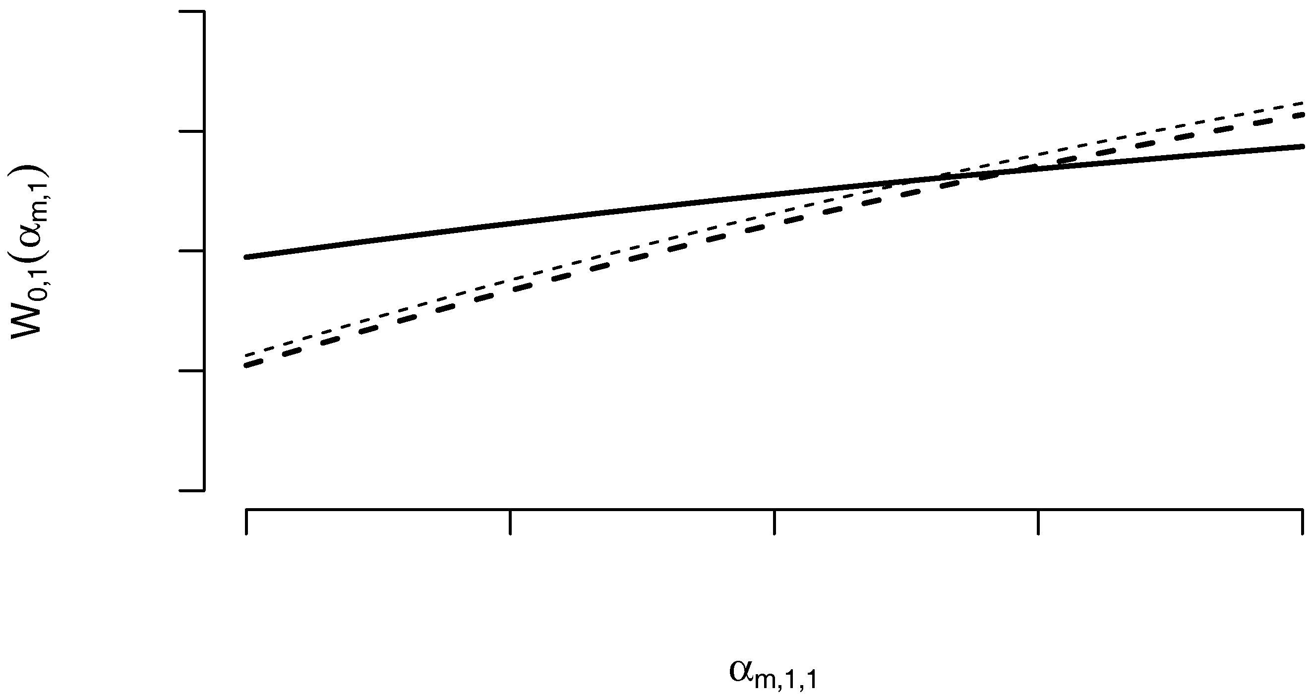
Figure 2 shows buyer’s demand in for different time horizons T. In the “flexible” case the WD prices are renegotiated at , and in the case no rebalancing takes place. From Figure 2 we observe that buyer’s demand price elasticity at is lower in the “flexible” case. Consistent with the classical result of Allen and Postlewaite (1984), already at individual demand reflects all agents’ expectations, including the expectations about future trading behaviour.
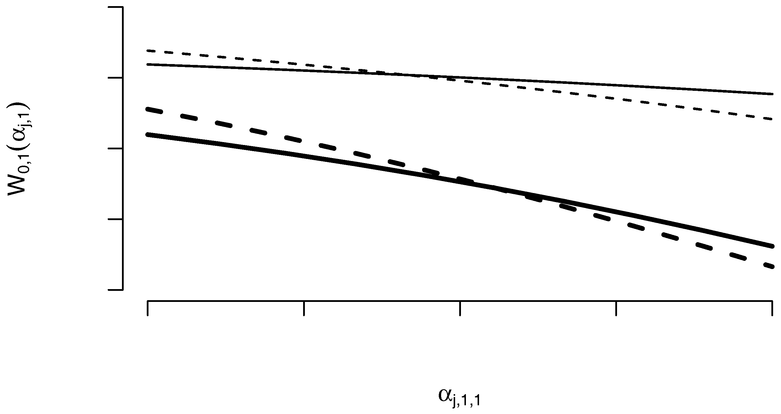
Figure 3 shows investor’s supply in for different time horizons T and for different levels in volatility of the alternative investment in the investor’s portfolio. In the “flexible” case the WD prices are renegotiated at , and in the case no rebalancing takes place. From Figure 3 we observe that the price elasticity of the investor’s supply at is lower in the “flexible” case. Moreover, the reaction of the supply to the changes in market volatility is very subtle in the “flexible” case (under 1% and is not visible in the graph), as the downward shift of the supply curve is quite pronounced for . In this case, increase in market volatility (or volatility of the alternative investment) significantly stimulates investor’s supply for WDs.
Our example shows pricing rainfall options. The presented pricing model, however, is not limited to any particular kind of weather derivatives. In fact, it is possible to price various weather derivatives with such underlying indices as snowfall, sunshine hours, number of sunny days, number of rainy days, wind speed, and other weather indices of a practical relevance for retail, tourism and renewable energy operators.
Along with the other assumptions, the premise is the existence of a probabilistic model that precisely enough describes the distribution and the time evolution of the underlying weather index. Then, the conditional expectations of agents’ utilities, which determine their supply and demand, can be approximated using Monte Carlo samples from the fitted probabilistic model. Applying partial market clearing condition, one obtains the equilibrium prices for weather derivatives.
4. Summary
We derive a dynamic utility-based model for pricing baskets of weather derivatives on multiple dependent underlying indices. Using dynamic programming approach to portfolio optimisation over a finite investment horizon and partial market clearing, we obtain semi-closed forms for the equilibrium prices of weather derivatives and for the optimal trading strategies. We provide extensions of the model to account for counterparty default risk and a possibility of an alternative financial investment.
As expected, there is an adverse effect of increasing default risk and capital costs on the demand for weather derivatives and on their prices. We find, however, a stimulating effect of increasing market volatility on the supply for weather derivatives.
We apply the proposed model to price rainfall options using historical rainfall data of agricultural provinces Changde and Enshi in China. The equilibrium put option prices on cumulative rainfall over May are compared for different market scenarios. The effects of increasing default risk, capital costs, investment horizon, and market volatility are assessed.
Acknowledgments
Authors acknowledge financial support of Deutsche Forschungsgemeinschaft through the CRC 649: Economic Risk.
Author Contributions
Wolfgang Karl Härdle and Maria Osipenko contributed equally to this work.
Conflicts of Interest
The authors declare no conflict of interest.The founding sponsors had no role in the design of the study; in the collection, analyses, or interpretation of data; in the writing of the manuscript, and in the decision to publish the results.
Appendix A
Proof of Proposition 1.
We prove the assertion by backward induction starting with . Utility maximisation problem of buyer j in :
The expected utility in reads:
By plugging the self-financing constraint in (A2) we obtain
Taking the first derivative of (A3) with respect to , we win the gradient vector with the sth entry equal to:
for . Taking the second derivative of (A3) with respect to gives the Hessian matrix H with th entry:
for . The Hessian H defined entry-wise by (A5) is negative semi-definite, since for any nonzero :
is always smaller or equal to zero. Hence, we obtain the maximiser of (A3) by setting the gradient (A4) coordinate-wise to zero, in particular:
In the current prices are known and can be taken out of the expectation in (A7). Thus, we obtain the reverse demand of the jth buyer for each as:
with .
Applying partial market clearing or zero-net-supply condition to all WDs, we find and . Then, the maximised utility of buyer j at is:
with
is of the exponential form like the utility function itself, and the induction hypothesis holds for . Assume, that it holds for . Then, in :
is the constrained utility maximisation problem faced by buyer j. The expected utility in is:
where
Now we use the following identity:
to rewrite (A12) as a function of :
By taking the derivative of (A15) with respect to we find the gradient with sth entry:
As in (A6) the Hessian is also negative semi-definite. Thus, the maximiser of (A15) is found by setting the gradient (A16) to zero, that is:
We obtain the reverse demand of the jth buyer for each as:
Partial market clearing in determines , and the maximised utility of buyer j in this period:
with
which completes the proof. ☐
References
- Alaton, Peter, Boalem Djehiche, and David Stillberger. 2002. On modelling and pricing weather derivatives. Applied Mathematical Finance 1: 1–20. [Google Scholar] [CrossRef]
- Allen, Franklin, and Andrew Postlewaite. 1984. Rational expectations and the measurement of a stock’s elasticity of demand. Journal of Finance 39: 1119–25. [Google Scholar] [CrossRef]
- Benth, Fred Espen, Jūrate Šaltyté Benth, and Steen Koekebakker. 2007. Putting a price on temperature. Scandinavian Journal of Statistics 34: 746–67. [Google Scholar] [CrossRef]
- Cao, Melanie, and Jason Wei. 2004. Pricing weather derivative: An equilibrium approach. Journal of Futures Markets 24: 1065–89. [Google Scholar] [CrossRef]
- Carmona, René, and Pavel Diko. 2005. Pricing precipitation based derivatives. International Journal of Theoretical and Applied Finance 8: 959–88. [Google Scholar] [CrossRef]
- Çanakoǧlu, Ethem, and Süleyman Özekici. 2009. Portfolio selection in stochastic markets with exponential utility functions. Annals of Operations Research 166: 281–97. [Google Scholar] [CrossRef]
- Chaumont, Sébastian, Peter Imkeller, and Matthias Müller. 2006. Equilibrium trading of climate and weather risk and numerical simulation in a Markovian framework. Stochastic Environment Research and Risk Assessment 20: 184–205. [Google Scholar] [CrossRef]
- Glauber, Joseph, Keith Collins, and Peter Barry. 2002. Crop insurance, disaster assistance, and the role of the federal government in providing catastrophic risk protection. Agricultural Finance Review 62: 81–101. [Google Scholar] [CrossRef]
- Golden, Linda, Mulong Wang, and Chuanhou Yang. 2007. Handling weather related risks through the financial markets: Considerations of credit risk, basis risk, and hedging. Journal of Risk & Insurance 74: 319–46. [Google Scholar]
- Heath, David, Robert Jarrow, and Andrew Morton. 1992. Bond pricing and the term structure of interest rates: A new methodology for contingent claims valuation. Econometrica 60: 77–105. [Google Scholar] [CrossRef]
- Horst, Ulrich, and Matthias Müller. 2007. On the spanning property of risk bonds priced by equilibrium. Mathematics of Operation Research 32: 784–807. [Google Scholar] [CrossRef]
- Hull, John, and Allan White. 1995. The impact of default risk on the prices of options and other derivative securities. Journal of Banking & Finance 19: 299–322. [Google Scholar]
- Jarrow, Robert A., and Stuart M. Turnbull. 1995. Pricing derivatives on financial securities subject to credit risk. Journal of Finance 50: 53–85. [Google Scholar] [CrossRef]
- Katz, Richard. 1981. On some criteria for estimating the order of a Markov chain. Technometrics 23: 243–49. [Google Scholar] [CrossRef]
- Lee, Yongheon, and Shmuel Oren. 2010. A multi-period equilibrium pricing model of weather derivatives. Energy Systems 1: 3–30. [Google Scholar] [CrossRef]
- Leobacher, Gunther, and Philip Ngare. 2011. On modelling and pricing rainfall derivatives with seasonality. Applied Mathematical Finance 18: 71–91. [Google Scholar] [CrossRef]
- López Cabrera, Brenda, Martin Odening, and Matthias Ritter. 2013. Pricing rainfall futures at the CME. Journal of Banking & Finance 37: 4286–98. [Google Scholar]
- Lucas, Robert E. 1978. Asset prices in an exchange economy. Econometrica 46: 1429–45. [Google Scholar] [CrossRef]
- Musshoff, Oliver, Martin Odening, and Wei Xu. 2010. Management of climate risks in agriculture—Will weather derivatives permeate? Applied Economics 43: 1067–77. [Google Scholar] [CrossRef]
- Pennacchi, George. 2008. Theory of Asset Pricing. Boston: Pearson Addison-Wesley. [Google Scholar]
- Peréz-González, Francisco, and Hayong Yun. 2013. Risk management and firm value: Evidence from weather derivatives. Journal of Finance 68: 2143–76. [Google Scholar] [CrossRef]
- Stokey, Nancy, Robert Lucas, and Edward Prescott. 1989. Recursive Methods in Economic Dynamics. Cambridge: Harvard University Press. [Google Scholar]
- The World Bank. 2007. China: Innovations in Agricultural Insurance—-Promoting Access to Agricultural Insurance for Small Farmers. Technical Report. Washington: The World Bank. [Google Scholar]
- Turvey, Calum, and Rong Kong. 2010. Weather risk and the viability of weather insurance in China’s Gansu, Shaanxi and Henan provinces. China Agricultural Economic Review 2: 5–24. [Google Scholar] [CrossRef]
- Wilks, Daniel. 1998. Multisite generalization of a daily stochastic precipitation generation model. Journal of Hydrology 210: 178–91. [Google Scholar] [CrossRef]
- Wu, Yang Che, and San Lin Chung. 2010. Catastrophe risk management with counterparty risk using alternative instruments. Insurance: Mathematics and Economics 47: 234–45. [Google Scholar] [CrossRef]
| 1. | Station numbers given by the World Meteorological Organisation are 57662 for Changde and 57447 for Enshi. |
Figure 1.
Shifts of the demand curves by increasing default risk (top) and capital costs (bottom).Top: the default risk probability changes from 0 (dashed) to 0.01, 0.05, 0.10 (solid lines, thicker with increasing p). Bottom: capital cost p.a. r changes from 1% (dashed) to 5%, 10%, 15% (solid lines, thicker with increasing r) for . Both plots: the x-axis shows , the buyer’s position in the put option on the rainfall in Changde during May () with strike and investment horizon ; the y-axis shows , the price our representative buyer is willing to pay for such an option, where and while , the position in the other put option on the rainfall in Enshi during May () is kept constant.
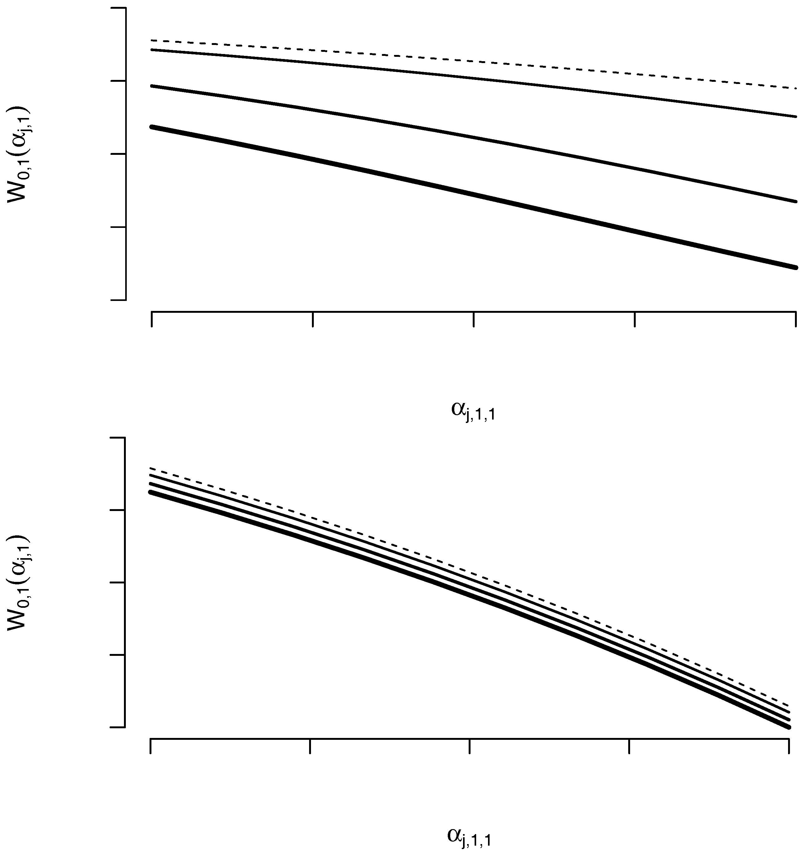
Figure 2.
Shifts of the demand curves by increasing investment horizon T. Buyer’s demand with investment horizon (dashed) and (solid). Thinner lines correspond to the case capital costs and probability of issuer’s default ; thicker lines correspond to capital costs and probability of issuer’s default for . The x-axis shows , the buyer’s position in the put option on the rainfall in Changde during May () with strike ; the y-axis shows , the price our representative buyer is willing to pay for such an option, where and while , the position in the other put option on the rainfall in Enshi during May () is kept constant.

Figure 3.
Shifts of the supply curves by increasing volatility of the alternative investment. Investor’s supply with investment horizon (dashed) and (solid). Thinner lines correspond to the case low volatility of the alternative investment; thicker lines correspond to high volatility. The x-axis shows , the investor’s position in the put option on the rainfall in Changde during May () with strike ; the y-axis shows , the price for which the investor is willing to sell such an option, where and while , the position in the other put option on the rainfall in Enshi during April and May () is kept constant.

Table 1.
Description of the rainfall data.
| Station | Number | Latitude | Longitude | Start Date | End Date |
|---|---|---|---|---|---|
| Changde | 57,662 | 29.05 | 111.68 | 1951/01/01 | 2009/11/30 |
| Enshi | 57,447 | 30.28 | 109.47 | 1951/08/01 | 2009/11/30 |
Table 2.
BIC criterion for different orders of Markov model for the rainfall occurrences in May
| Order/BIC | Changde | Enshi |
|---|---|---|
| 0 | 70.83 | 60.02 |
| 1 | 53.21 | 43.21 |
| 2 | 53.47 | 44.69 |
| 3 | 65.64 | 59.72 |
Table 3.
Maximum Likelihood estimator for the mixture of two exponential distributions for the rainfall amounts.
Table 3.
Maximum Likelihood estimator for the mixture of two exponential distributions for the rainfall amounts.
| Parameter | Changde | Enshi |
|---|---|---|
| 0.78 | 0.58 | |
| 15.90 | 23.14 | |
| 0.62 | 1.86 |
Table 4.
Put option prices on cumulative rainfall in Changde and Enshi under different market scenarios.
Table 4.
Put option prices on cumulative rainfall in Changde and Enshi under different market scenarios.
| Scenarios | Put on | Put on | ||||
|---|---|---|---|---|---|---|
| 100.00 | 100.30 | 100.00 | 96.68 | |||
| 99.67 | 99.95 | 98.81 | 96.35 | |||
| 91.22 | 93.95 | 86.74 | 87.45 | |||
| 90.87 | 93.62 | 85.95 | 87.12 | |||
| 100.00 | 100.31 | 100.23 | 96.68 | |||
| 99.67 | 99.97 | 99.71 | 96.36 | |||
| 91.23 | 94.23 | 86.88 | 87.73 | |||
| 90.92 | 93.99 | 86.47 | 87.51 | |||
© 2017 by the authors. Licensee MDPI, Basel, Switzerland. This article is an open access article distributed under the terms and conditions of the Creative Commons Attribution (CC BY) license (http://creativecommons.org/licenses/by/4.0/).
Share and Cite
MDPI and ACS Style
Härdle, W.K.; Osipenko, M. A Dynamic Programming Approach for Pricing Weather Derivatives under Issuer Default Risk. Int. J. Financial Stud. 2017, 5, 23. https://doi.org/10.3390/ijfs5040023
AMA Style
Härdle WK, Osipenko M. A Dynamic Programming Approach for Pricing Weather Derivatives under Issuer Default Risk. International Journal of Financial Studies. 2017; 5(4):23. https://doi.org/10.3390/ijfs5040023
Chicago/Turabian StyleHärdle, Wolfgang Karl, and Maria Osipenko. 2017. "A Dynamic Programming Approach for Pricing Weather Derivatives under Issuer Default Risk" International Journal of Financial Studies 5, no. 4: 23. https://doi.org/10.3390/ijfs5040023
Note that from the first issue of 2016, this journal uses article numbers instead of page numbers. See further details here.