Numerical Simulation of the Heston Model under Stochastic Correlation

Abstract

Stochastic correlation models have become increasingly important in financial markets. In order to be able to price vanilla options in stochastic volatility and correlation models, in this work, we study the extension of the Heston model by imposing stochastic correlations driven by a stochastic differential equation. We discuss the efficient algorithms for the extended Heston model by incorporating stochastic correlations. Our numerical experiments show that the proposed algorithms can efficiently provide highly accurate results for the extended Heston by including stochastic correlations. By investigating the effect of stochastic correlations on the implied volatility, we find that the performance of the Heston model can be proved by including stochastic correlations.

1. Introduction

The Heston Model Heston (1993) is one of the most widely used stochastic volatility models. It is an extension of the Black–Scholes (Black and Scholes 1973) model by taking into account stochastic volatility given by the Cox–Ingersoll–Ross (CIR) process. The attractiveness of the Heston model is its analytical tractability and the consideration of the correlation between the underlying asset price process and volatility process. Subsequently, a couple of papers on the numerically stable and efficient computation of European-style option prices were published, e.g., (Andersen 2008; Carr and Madan 1999; Kahl and Jäckel 2005; Lee 2004; Lewis 2001; Lipton 2002).

It has been pointed out, in many works (see, e.g., (Christoffersen et al. 2009; Grzelak and Oosterlee 2011)) that the Heston model is unable to provide enough skew in the implied volatility as market required, especially for a short maturity. Therefore, one tries to extend the Heston model. For example, one way is to extend the Heston by introducing a more realistic stochastic volatility process, which is the double Heston model (Christoffersen et al. 2009) or by introducing a stochastic interest rate, which is the Hybrid–Heston–Hull–White model (HHW) (Grzelak and Oosterlee 2011); another way is to adapt the Heston model by allowing time-dependent parameters (see Elices 2009; Mikhailov and Nögel 2003). Actually, the major factor that affects the implied volatility skew is the correlation. However, in the pure Heston model (Heston 1993), and also in most of the extended Heston models, only a constant correlation coefficient is used. It has been shown in Teng et al. (2014b, 2016b) that the calibration to market data can be already improved by allowing a local time-dependent correlation model. Therefore, in this work, we extend the Heston model by imposing a stochastic correlation model cf. Emmerich (2006); Teng et al. (2014a, 2016a) and discuss its simulation methods. Furthermore, using Monte Carlo simulation, we study how the implied volatility is affected by introducing stochastic correlations.

In the next section, we impose a stochastic correlation model to the Heston model and discuss in Section 3 a discretization for each path of the variance, correlation and the log price process including numerical analysis. Section 4 is devoted to firstly comparing different numerical algorithms, and secondly to recognizing the effect of imposing stochastic correlation on implied volatility. Finally, Section 5 concludes this work.

2. Stochastic Correlation in the Heston Model

We study the Heston model and its extension by incorporating a stochastic correlation process. Heston’s stochastic volatility model under the risk-neutral measure reads

$$\begin{array}{cc}\hfill d{S}_t& =r{S}_{t}dt+\sqrt{{\nu }_t}{S}_{t}d{W}_t^S,\hfill \end{array}$$

(1)

$$\begin{array}{cc}\hfill d{\nu }_t& ={\kappa }_{\nu }({\mu }_{\nu }-{\nu }_t)dt+{\sigma }_{\nu }\sqrt{{\nu }_t}d{W}_t^{\nu },\hfill \end{array}$$

(2)

where $S_t$ denotes the spot price of the asset and ${\nu }_t$ is the instantaneous variance, where ${\mu }_{\nu }$ is the long-term variance, ${\kappa }_{\nu }$ is the speed at which it reverts to ${\mu }_{\nu }$ and ${\sigma }_{\nu }$ is the volatility of the variance process. We note that the process (2) is strictly positive if the parameters obey the Feller condition $2{\kappa }_{\nu }{\mu }_{\nu }>{\sigma }_{\nu }$. The Brownian motions (BMs) $W^S$ and $W^{\nu }$ are correlated with a constant ${\rho }_{S\nu }$ by

$$d{W}_t^{S}d{W}_t^{\nu }={\rho }_{S\nu }dt$$

(3)

and under risk-neutral measure. By applying Itô’s Lemma with $x_t=log\left(S_t\right)$ (log-transform), we obtain from (1) the log price process as

$$d{x}_t=(r-\frac{1}{2}{\nu }_t)dt+\sqrt{{\nu }_t}d{W}_t^x,$$

(4)

where $W_t^x$ is the same BM to $W_t^S$ in (1). We suppose an appropriate stochastic correlation process of the form

$$d{\rho }_t=\tilde{a}(t,{\rho }_t)dt+\tilde{b}(t,{\rho }_t)d{\tilde{W}}_t^{\rho },$$

(5)

where $\tilde{a}(t,{\rho }_t)$ and $\tilde{b}(t,{\rho }_t)$ are given functions depending on the chosen correlation process, ${\tilde{W}}_t^{\rho }$ is a standard BM with respect to the physical measure. By including the market price of correlation risk, the correlation process (5) can be rewritten as

$$d{\rho }_t=(\tilde{a}(t,{\rho }_t)-\lambda (S_t,{\nu }_t,{\rho }_t,t))dt+\tilde{b}(t,{\rho }_t)d{W}_t^{\rho },$$

(6)

which is under risk-neutral measure, where $\lambda (S_t,{\nu }_t,{\rho }_t,t)$ represents the price of the correlation risk and could be assumed to be $\lambda {\rho }_t$, with a constant $\lambda$. In what follows, we set $\tilde{a}(t,{\rho }_t)-\lambda (S_t,{\nu }_t,{\rho }_t,t)=a(t,{\rho }_t)$ and $b(t,{\rho }_t)=\tilde{b}(t,{\rho }_t)$. With the aim of imposing a stochastic correlation between the log price process $d{x}_t$ and the stochastic variance $d{\nu }_t$, we extend the Heston model as

$$\begin{array}{cc}\hfill d{\nu }_t& ={\kappa }_{\nu }({\mu }_{\nu }-{\nu }_t)dt+{\sigma }_{\nu }\sqrt{{\nu }_t}d{W}_t^{\nu },\hfill \end{array}$$

(7)

$$\begin{array}{cc}\hfill d{\rho }_t& =a(t,{\rho }_t)dt+b(t,{\rho }_t)d{W}_t^{\rho },\hfill \end{array}$$

(8)

$$\begin{array}{cc}\hfill d{x}_t& =(r-\frac{1}{2}{\nu }_t)dt+\sqrt{{\nu }_t}d{W}_t^x,\hfill \end{array}$$

(9)

with

$$d{W}^{x}d{W}^{\nu }={\rho }_{t}dt,d{W}^{x}d{W}^{\rho }={\rho }^{x\rho }dt,d{W}^{\nu }d{W}^{\rho }={\rho }^{\nu \rho }dt,$$

(10)

where ${\rho }_t$ is given by (8), and ${\rho }^{x\rho }$ and ${\rho }^{\nu \rho }$ are assumed to be two constant correlations.

3. Path Simulation

We now discuss how to simulate the paths for (7)–(9) to compute the price of European options in the extended Heston model applying Monte Carlo simulation. We need to generate random paths of the triplet $({\nu }_t,{\rho }_t,x_t)$ for all $t\in {\left\{t_i\right\}}_{i=1}^N:=\mathcal{T}$. To be more precise, for an arbitrary time increment $\mathsf{\Delta }$, we need to generate a random sample of $({\nu }_{t+\mathsf{\Delta }},{\rho }_{t+\mathsf{\Delta }},x_{t+\mathsf{\Delta }})$ for given $({\nu }_t,{\rho }_t,x_t)$. Repeated application of the resulting one period scheme will generate a full path ${({\nu }_t,{\rho }_t,x_t)}_{t\in \mathcal{T}}$.

3.1. Discretization for the Variance Process ${\nu }_t$

To discretize the variance process ${\nu }_t$, we employ the quadratic-exponential (QE) scheme by Andersen (2008). The idea of the QE scheme is the approximation to the non-central chi-square distribution. Let ${\widehat{\nu }}_t$ denote a discrete-time approximation to ${\nu }_t$, for sufficiently large realized values of ${\widehat{\nu }}_t$, Andersen (2008) suggested to approximate the non-central chi-square random variable by the power function

$${\widehat{\nu }}_{t+\mathsf{\Delta }}=\alpha {(\beta +Z^{\nu })}^2,$$

(11)

where $Z^{\nu }$ is a standard Gaussian random variable, $\alpha$ and $\beta$ are certain constants that can be determined by moment-matching using the parameters in (7) and given in the following Proposition 1; the detailed calculations can be found in Andersen (2008).

Proposition 1.

The mean and the variance of the variance process (7) read

$$\begin{array}{cc}\hfill m& =E\left[{\nu }_{t+\mathsf{\Delta }}\right|{\nu }_t]={\mu }_{\nu }+({\nu }_t-{\mu }_{\nu }){\mathrm{e}}^{-{\kappa }_{\nu }(T-t)},\hfill \end{array}$$

(12)

$$\begin{array}{cc}\hfill s^2& =\frac{{\nu }_t{\sigma }_{\nu }^2{\mathrm{e}}^{-{\kappa }_{\nu }(T-t)}}{{\kappa }_{\nu }}\left(1-e^{-{\kappa }_{\nu }(T-t)}\right)+\frac{{\mu }_{\nu }{\sigma }_{\nu }^2}{2{\kappa }_{\nu }}{\left(1-e^{-{\kappa }_{\nu }(T-t)}\right)}^2.\hfill \end{array}$$

(13)

If we set $\psi :=\frac{s^2}{m^2}$ and choose

$${\beta }^2=2{\psi }^{-1}-1+\sqrt{2{\psi }^{-1}}\sqrt{2{\psi }^{-1}-1}\ge 0$$

(14)

and

$$\alpha =\frac{m}{1+{\beta }^2},$$

(15)

then (11) has a mean equal to m and a variance equal to $s^2$. Note that $\psi \le 2$.

However, the approximation (11) will not work well for small values of ${\widehat{\nu }}_t$, cf. Andersen (2008). For small values of ${\widehat{\nu }}_t$, Andersen (2008) suggested to use an approximated density for ${\widehat{\nu }}_{t+\mathsf{\Delta }}$ of the form:

$$P({\widehat{\nu }}_{t+\mathsf{\Delta }}\in [x,x+dx])\approx (p\delta \left(0\right)+q(1-p){\mathrm{e}}^{-qx})dx,x\ge 0,$$

(16)

where $\delta$ is a Dirac delta function, and $p\in [0,1]$ and $q>0$ are constants to be determined by moment-matching. We integrate (16) and obtain

$$\mathsf{\Psi }\left(x\right)=P({\widehat{\nu }}_{t+\mathsf{\Delta }}<x)=p+(1-p)(1-{\mathrm{e}}^{-qx}),x\ge 0$$

(17)

and, by inverting, we obtain

$${\mathsf{\Psi }}^{-1}\left(u\right)={\mathsf{\Psi }}^{-1}(u;p,q)=\left\{\begin{array}{cc}0,\hfill & 0\le u\le p,\hfill \\ q^{-1}ln\left(\frac{1-p}{1-u}\right),\hfill & p<u\le 1.\hfill \end{array}\right.$$

(18)

Thus, the sampling scheme for small values of ${\widehat{\nu }}_t$ reads

$${\widehat{\nu }}_{t+\mathsf{\Delta }}={\mathsf{\Psi }}^{-1}(U^{\nu };p,q),$$

(19)

where $U^{\nu }$ is a uniform random variable.

Proposition 2.

Let m, $s^2$ and ψ be defined as in Proposition 1. For $\psi \ge 1$, there exist two parameters p and q such that (19) has a mean equal to m and a variance equal to $s^2$, which read

$$p=\frac{\psi -1}{\psi +1}\in [0,1)$$

(20)

and

$$q=\frac{1-p}{m}=\frac{2}{m(\psi +1)}>0.$$

(21)

We only need to select an arbitrary level ${\psi }_c\in [1,2]$ and choose either (11) or (19) according to $\psi \le {\psi }_c$ or $\psi >{\psi }_c$ to do the sampling for the variance process (7).

3.2. Discretization for the Correlation Process ${\rho }_t$

We know that several stochastic processes could be used for modelling stochastic correlation, e.g., the bounded Jacobi process (Ma 2009; Emmerich 2006), the sort of stochastic correlation process produced by transformation (Teng et al. 2014a, 2016a). Moreover, for nice analytical tractability, we might choose some other mean-reverting processes that exhibit simpler structure, e.g., the Ornstein–Uhlenbeck (OU) process (Uhlenbeck and Ornstein 1930).

$$d{\rho }_t={\kappa }_{\rho }({\mu }_{\rho }-{\rho }_t)dt+{\sigma }_{\rho }d{W}_t^{\rho }$$

(22)

with the exact solution

$${\rho }_{t+\mathsf{\Delta }}={\rho }_t{\mathrm{e}}^{-{\kappa }_{\rho }\mathsf{\Delta }}+{\mu }_{\rho }(1-{\mathrm{e}}^{-{\kappa }_{\rho }\mathsf{\Delta }})+{\sigma }_{\rho }\sqrt{\frac{1-{\mathrm{e}}^{-2{\kappa }_{\rho }\mathsf{\Delta }}}{2{\kappa }_{\rho }}}{Z}^{\rho },$$

(23)

where $Z^{\rho }$ is a standard Gaussian random variable. Thus, the functions $a(t,{\rho }_t)$ and $b(t,{\rho }_t)$ defined in (5) are known as ${\kappa }_{\rho }({\mu }_{\rho }-{\rho }_t)$ and ${\sigma }_{\rho }$, respectively. However, the major drawback of using the OU process for stochastic correlation is that the process is not bounded. This is to say the generated correlations can be out of the correlation interval $[-1,1]$, especially with a small value of ${\kappa }_{\rho }$ and a large value of ${\sigma }_{\rho }$. Moreover, it has been indicated by Teng et al. in (Teng et al. 2016b) that $P({\rho }_t<1)=1$ is valid if and only if

$$\frac{\sqrt{{\kappa }_{\rho }}(1-{\mu }_{\rho })}{{\sigma }_{\rho }}\to \infty ,$$

(24)

and the condition for $P({\rho }_t>-1)=1$ is

$$\frac{\sqrt{{\kappa }_{\rho }}(-1-{\mu }_{\rho })}{{\sigma }_{\rho }}\to -\infty .$$

(25)

This does not necessarily means that ${\sigma }_{\rho }$ tends to zero. If one limits the mean value ${\mu }_{\rho }$ to be in $(-1,1)$, from (24) and (25), one can conclude that the OU process is bounded in the interval with the condition $\frac{\sqrt{{\kappa }_{\rho }}}{{\sigma }_{\rho }}\to \infty$. In practice, such a positive constant C could be selected such that the condition $\frac{\sqrt{{\kappa }_{\rho }}}{{\sigma }_{\rho }}\ge C$ is already sufficient to ensure that the generated correlations stay in $(-1,1)$, if the initial correlation ${\rho }_0$ and the long-term mean ${\mu }_{\rho }$ are not close to $-1$ or 1.

3.3. Discretization for the Log Price Process $x_t$

In this section, we discuss how to discretize the log price process (9). As indicated by Andersen (2008), a straight discretization of (9) may lead to the problem of “leaking correlation”: suppose that we use directly a Euler scheme for simulating (9):

$${\widehat{x}}_{t+\mathsf{\Delta }}={\widehat{x}}_t+(r-\frac{1}{2}{\widehat{\nu }}_t)\mathsf{\Delta }+\sqrt{{\widehat{\nu }}_t}{Z}_x\sqrt{\mathsf{\Delta }}.$$

(26)

We know that the true correlation between ${\widehat{x}}_{t+\mathsf{\Delta }}$ and ${\widehat{\nu }}_{t+\mathsf{\Delta }}$ is always close to ${\rho }_t$ given by (8). However, ${\widehat{\nu }}_{t+\mathsf{\Delta }}$ and $Z_{\nu }$ in (11) have a strong nonlinear relationship, which will imply that the effective correlation between ${\widehat{x}}_{t+\mathsf{\Delta }}$ and ${\widehat{\nu }}_{t+\mathsf{\Delta }}$ will be closer to zero than ${\rho }_t$ for the cases where the probability $P(\beta +Z_v<0)$ is nonzero. To tackle this problem of “leaking correlation”, we reformulate the stochastic differential equation (SDE) system (7)–(9) as follows: first, we see that the SDE system (7)–(9) has a family of correlation matrices

$${\mathcal{C}}_t=\left(\begin{array}{ccc}1& {\rho }^{\nu \rho }& {\rho }_t\\ {\rho }^{\rho \nu }& 1& {\rho }^{\rho x}\\ {\rho }_t& {\rho }^{x\rho }& 1\end{array}\right),t\ge 0.$$

(27)

To simplify notation, we set ${\rho }_1:={\rho }^{\nu \rho }\left({\rho }^{\rho \nu }\right)$ and ${\rho }_2:={\rho }^{x\rho }\left({\rho }^{\rho x}\right)$. One can thus perform a Cholesky-decomposition ${\mathcal{C}}_t={\mathcal{L}}_t{\mathcal{L}}_t^{\top }$, where ${\mathcal{L}}_t$ is a family of lower triangular matrices given by

$${\mathcal{L}}_t=\left(\begin{array}{ccc}1& 0& 0\\ {\rho }_1& \sqrt{1-{\rho }_1^2}& 0\\ {\rho }_t& \frac{{\rho }_2-{\rho }_1{\rho }_t}{\sqrt{1-{\rho }_1^2}}& \sqrt{1-{\rho }_t^2-{\left(\frac{{\rho }_2-{\rho }_1{\rho }_t}{\sqrt{1-{\rho }_1^2}}\right)}^2}\end{array}\right),t\ge 0,$$

(28)

which can be used to reformulate the SDE system (7)–(9) with respect to the independent BMs ${\tilde{W}}_t^{\nu },{\tilde{W}}_t^{\rho }$ and ${\tilde{W}}_t^x$ as:

$$\begin{array}{cc}\hfill d{\nu }_t& ={\kappa }_{\nu }({\mu }_{\nu }-{\nu }_t)dt+{\sigma }_{\nu }\sqrt{{\nu }_t}d{\tilde{W}}_t^{\nu },\hfill \end{array}$$

(29)

$$\begin{array}{cc}\hfill d{\rho }_t& =a(t,{\rho }_t)dt+{\rho }_{1}b(t,{\rho }_t)d{\tilde{W}}_t^{\nu }+\sqrt{1-{\rho }_1^2}b(t,{\rho }_t)d{\tilde{W}}_t^{\rho },\hfill \end{array}$$

(30)

$$\begin{array}{c}d{x}_t=(r-\frac{1}{2}{\nu }_t)dt+{\rho }_t\sqrt{{\nu }_t}d{\tilde{W}}_t^{\nu }+\frac{{\rho }_2-{\rho }_1{\rho }_t}{\sqrt{1-{\rho }_1^2}}\sqrt{{\nu }_t}d{\tilde{W}}_t^{\rho }\hfill \\ +\sqrt{1-{\rho }_t^2-{\left(\frac{{\rho }_2-{\rho }_1{\rho }_t}{\sqrt{1-{\rho }_1^2}}\right)}^2}\sqrt{{\nu }_t}d{\tilde{W}}_t^x.\hfill \end{array}$$

(31)

Since our main aim is to impose a stochastic correlation between the asset process (31) and the stochastic variance process (29), to simplify the model, we assume ${\rho }_1=0$, and the latter SDE system thus becomes

$$\begin{array}{cc}\hfill d{\nu }_t& ={\kappa }_{\nu }({\mu }_{\nu }-{\nu }_t)dt+{\sigma }_{\nu }\sqrt{{\nu }_t}d{\tilde{W}}_t^{\nu },\hfill \end{array}$$

(32)

$$\begin{array}{cc}\hfill d{\rho }_t& =a(t,{\rho }_t)dt+b(t,{\rho }_t)d{\tilde{W}}_t^{\rho },\hfill \end{array}$$

(33)

$$\begin{array}{cc}\hfill d{x}_t& =(r-\frac{1}{2}{\nu }_t)dt+{\rho }_t\sqrt{{\nu }_t}d{\tilde{W}}_t^{\nu }+{\rho }_2\sqrt{{\nu }_t}d{\tilde{W}}_t^{\rho }+\sqrt{1-{\rho }_t^2-{\rho }_2^2}\sqrt{{\nu }_t}d{\tilde{W}}_t^x.\hfill \end{array}$$

(34)

In the following, we will discuss two different ways to discretize (34).

3.3.1. The Euler and Milstein Scheme (EM Scheme)

The most simple way of discretizing (34) is to use the Euler or Milstein scheme. The discretization of (34) by applying the Euler scheme (Euler [1768] 1913; Maruyama 1955) reads

$$\begin{array}{c}{\widehat{x}}_{t+\mathsf{\Delta }}={\widehat{x}}_t+(r-\frac{1}{2}{\widehat{\nu }}_t)\mathsf{\Delta }+{\rho }_2\sqrt{\mathsf{\Delta }}{Z}^{\tilde{\rho }}\sqrt{{\widehat{\nu }}_t}+{\widehat{\rho }}_t\sqrt{\mathsf{\Delta }}{Z}^{\tilde{\nu }}\sqrt{{\widehat{\nu }}_t}+\sqrt{1-{\rho }_2^2-{\tilde{\rho }}_t^2}\sqrt{\mathsf{\Delta }}{Z}^{\tilde{x}}\sqrt{{\widehat{\nu }}_t},\end{array}$$

(35)

where $Z^{\tilde{\rho }},Z^{\tilde{\nu }}$ and $Z^{\tilde{x}}$ are independent standard Gaussian random variables. The discretization of (34) by applying the Milstein scheme Milstein (1974) will be the same to (35), since all the derivatives included in the coefficients of the double integral terms (with respect to BMs) by the Milstein scheme are equal to zero. Moreover, we remark that ${\widehat{S}}_t=exp\left({\widehat{x}}_t\right)$ with the discretized process ${\widehat{x}}_t$ in (35) is a martingale, and any types of stochastic correlation processes can be straightforwardly employed within this scheme.

3.3.2. The Hybrid Scheme (HB Scheme)

In this section, we introduce a new way to discretize (34) where several different approximation techniques will be used. We thus call it the hybrid scheme. We take the OU process as an example due to its analytical tractability and start with the integral form of (34)

$$\begin{array}{c}{x}_{t+\mathsf{\Delta }}=x_t+r\mathsf{\Delta }-\frac{1}{2}{\int }_t^{t+\mathsf{\Delta }}{\nu }_{u}du+{\int }_t^{t+\mathsf{\Delta }}{\rho }_u\sqrt{{\nu }_u}d{\tilde{W}}_u^{\nu }+{\rho }_2{\int }_t^{t+\mathsf{\Delta }}\sqrt{{\nu }_u}d{\tilde{W}}_u^{\rho }+{\int }_t^{t+\mathsf{\Delta }}\sqrt{1-{\rho }_u^2-{\rho }_2^2}\sqrt{{\nu }_u}d{\tilde{W}}_u^x,\end{array}$$

(36)

where ${\rho }_t$ follows an OU process. For the integral ${\int }_t^{t+\mathsf{\Delta }}{\rho }_u\sqrt{{\nu }_u}d{\tilde{W}}_u^{\nu }$, where the integrand is not independent from the corresponding BM, we consider Itô’s product in the following

$$d{\rho }_t{\nu }_t={\rho }_t{\kappa }_{\nu }({\mu }_{\nu }-{\nu }_t)dt+{\nu }_t{\kappa }_{\rho }({\mu }_{\rho }-{\rho }_t)dt+{\nu }_t{\sigma }_{\rho }d{\tilde{W}}_t^{\rho }+{\rho }_t{\sigma }_{\nu }\sqrt{{\nu }_t}d{\tilde{W}}_t^{\nu },$$

(37)

where it has been assumed that ${\nu }_t$ and ${\rho }_t$ are independent from each other corresponding to ${\rho }_1=0$. This product implies that

$$\begin{array}{cc}{\int }_t^{t+\mathsf{\Delta }}{\rho }_u\sqrt{{\nu }_u}d{\tilde{W}}_u^{\nu }& =\frac{{\rho }_{t+\mathsf{\Delta }}{\nu }_{t+\mathsf{\Delta }}}{{\sigma }_{\nu }}-\frac{{\rho }_t{\nu }_t}{{\sigma }_{\nu }}-\frac{{\sigma }_{\rho }}{{\sigma }_{\nu }}{\int }_t^{t+\mathsf{\Delta }}{\nu }_{u}d{\tilde{W}}_u^{\rho }\hfill \\ & -{\int }_t^{t+\mathsf{\Delta }}\frac{{\kappa }_{\nu }{\mu }_{\nu }{\rho }_u+{\kappa }_{\rho }{\mu }_{\rho }{\nu }_u-({\kappa }_{\nu }+{\kappa }_{\rho }){\rho }_u{\nu }_u}{{\sigma }_{\nu }}du.\hfill \end{array}$$

(38)

Now, we insert (38) into (36)

$$\begin{array}{cc}\hfill x_{t+\mathsf{\Delta }}=x_t+r\mathsf{\Delta }& -\frac{1}{2}{\int }_t^{t+\mathsf{\Delta }}{\nu }_{u}du+\frac{{\rho }_{t+\mathsf{\Delta }}{\nu }_{t+\mathsf{\Delta }}}{{\sigma }_{\nu }}-\frac{{\rho }_t{\nu }_t}{{\sigma }_{\nu }}\hfill \\ & -{\int }_t^{t+\mathsf{\Delta }}\frac{{\kappa }_{\nu }{\mu }_{\nu }{\rho }_u+{\kappa }_{\rho }{\mu }_{\rho }{\nu }_u-({\kappa }_{\nu }+{\kappa }_{\rho }){\rho }_u{\nu }_u}{{\sigma }_{\nu }}du\hfill \\ & +{\int }_t^{t+\mathsf{\Delta }}{\rho }_2\sqrt{{\nu }_u}d{\tilde{W}}_u^{\rho }-{\int }_t^{t+\mathsf{\Delta }}\frac{{\sigma }_{\rho }}{{\sigma }_{\nu }}{\nu }_{u}d{\tilde{W}}_u^{\rho }+{\int }_t^{t+\mathsf{\Delta }}\sqrt{1-{\rho }_u^2-{\rho }_2^2}\sqrt{{\nu }_u}d{\tilde{W}}_u^x.\hfill \end{array}$$

(39)

For the integrals over the time in (39), we simply use the approximation

$$\mathsf{\Delta }\left({\gamma }_1{\nu }_t+{\gamma }_2{\nu }_{t+\mathsf{\Delta }}\right),$$

(40)

and

$$\begin{array}{c}\hfill \mathsf{\Delta }\left({\gamma }_1\frac{{\kappa }_{\nu }{\mu }_{\nu }{\rho }_t+{\kappa }_{\rho }{\mu }_{\rho }{\nu }_t-({\kappa }_{\nu }+{\kappa }_{\rho }){\rho }_t{\nu }_t}{{\sigma }_{\nu }}\right.\left.+{\gamma }_2\frac{{\kappa }_{\nu }{\mu }_{\nu }{\rho }_{t+\mathsf{\Delta }}+{\kappa }_{\rho }{\mu }_{\rho }{\nu }_{t+\mathsf{\Delta }}-({\kappa }_{\nu }+{\kappa }_{\rho }){\rho }_{t+\mathsf{\Delta }}{\nu }_{t+\mathsf{\Delta }}}{{\sigma }_{\nu }}\right),\end{array}$$

(41)

where ${\gamma }_1$ and ${\gamma }_2$ are given constants, e.g., we choose ${\gamma }_1={\gamma }_2=\frac{1}{2}$ for a central discretization.

In all the Itô integrals in (39), the integrand is independent with the corresponding BM. Thus, they can be approximated by

$${\int }_t^{t+\mathsf{\Delta }}\left({\rho }_2\sqrt{{\nu }_u}-\frac{{\sigma }_{\rho }}{{\sigma }_{\nu }}{\nu }_u\right)d{\tilde{W}}_u^{\rho }\approx \sqrt{\mathsf{\Delta }}\sqrt{{\gamma }_1{\left({\rho }_2\sqrt{{\nu }_t}-\frac{{\sigma }_{\rho }}{{\sigma }_{\nu }}{\nu }_t\right)}^2+{\gamma }_2{\left({\rho }_2\sqrt{{\nu }_{t+\mathsf{\Delta }}}-\frac{{\sigma }_{\rho }}{{\sigma }_{\nu }}{\nu }_{t+\mathsf{\Delta }}\right)}^2}{Z}^{\tilde{\rho }},$$

(42)

and

$${\int }_t^{t+\mathsf{\Delta }}\sqrt{1-{\rho }_u^2-{\rho }_2^2}\sqrt{{\nu }_u}d{\tilde{W}}_u^x\approx \sqrt{\mathsf{\Delta }}\sqrt{{\gamma }_1{\nu }_t\left(1-{\rho }_t^2-{\rho }_2^2\right)+{\gamma }_2{\nu }_{t+\mathsf{\Delta }}\left(1-{\rho }_{t+\mathsf{\Delta }}^2-{\rho }_2^2\right)}{Z}^{\tilde{x}},$$

(43)

respectively, where $Z^{\tilde{\rho }}$ and $Z^{\tilde{x}}$ are independent standard Gaussian random variables. With all the approximations mentioned above, we rearrange (39) as

$$\begin{array}{cc}\hfill {\widehat{x}}_{t+\mathsf{\Delta }}={\widehat{x}}_t+r\mathsf{\Delta }& +K_1{\nu }_t+K_2{\widehat{\nu }}_{t+\mathsf{\Delta }}+K_3{\widehat{\rho }}_t{\widehat{\nu }}_t+K_4{\widehat{\rho }}_{t+\mathsf{\Delta }}{\widehat{\nu }}_{t+\mathsf{\Delta }}+K_5{\widehat{\rho }}_t+K_6{\widehat{\rho }}_{t+\mathsf{\Delta }}\hfill \\ & +\sqrt{K_{\nu }^1{\widehat{\nu }}_t+K_{\nu }^2{\widehat{\nu }}_t^{\frac{3}{2}}+K_{\nu }^3{\widehat{\nu }}_t^2+K_{\nu }^4{\widehat{\nu }}_{t+\mathsf{\Delta }}+K_{\nu }^5{\widehat{\nu }}_{t+\mathsf{\Delta }}^{\frac{3}{2}}+K_{\nu }^6{\widehat{\nu }}_{t+\mathsf{\Delta }}^2}{Z}^{\tilde{\rho }}\hfill \\ & +\sqrt{K_{\rho }^1{\widehat{\nu }}_t+K_{\rho }^2{\widehat{\nu }}_t{\widehat{\rho }}_t^2+K_{\rho }^3{\widehat{\nu }}_{t+\mathsf{\Delta }}+K_{\rho }^4{\widehat{\nu }}_{t+\mathsf{\Delta }}{\widehat{\rho }}_{t+\mathsf{\Delta }}^2}{Z}^{\tilde{x}},\hfill \end{array}$$

(44)

where

$$\begin{array}{l}{K}_1:=-\mathsf{\Delta }{\gamma }_1\left(\frac{{\kappa }_{\rho }{\mu }_{\rho }}{{\sigma }_{\nu }}+\frac{1}{2}\right),K_2:=-\mathsf{\Delta }{\gamma }_2\left(\frac{{\kappa }_{\rho }{\mu }_{\rho }}{{\sigma }_{\nu }}+\frac{1}{2}\right),\\ K_3:=\frac{1}{{\sigma }_{\nu }}\left(\mathsf{\Delta }{\gamma }_1({\kappa }_{\nu }+{\kappa }_{\rho })-1\right),K_4:=\frac{1}{{\sigma }_{\nu }}\left(\mathsf{\Delta }{\gamma }_2({\kappa }_{\nu }+{\kappa }_{\rho })+1\right),\\ K_5:=-\frac{\mathsf{\Delta }{\gamma }_1{\kappa }_{\nu }{\mu }_{\nu }}{{\sigma }_{\nu }},K_6:=-\frac{\mathsf{\Delta }{\gamma }_2{\kappa }_{\nu }{\mu }_{\nu }}{{\sigma }_{\nu }},\\ K_{\nu }^1:=\mathsf{\Delta }{\gamma }_1{\rho }_2^2,K_{\nu }^2:=-\frac{2\mathsf{\Delta }{\gamma }_1{\rho }_2{\sigma }_{\rho }}{{\sigma }_{\nu }},K_{\nu }^3:=\frac{\mathsf{\Delta }{\gamma }_1{\sigma }_{\rho }^2}{{\sigma }_{\nu }^2},\\ K_{\nu }^4:=\mathsf{\Delta }{\gamma }_2{\rho }_2^2,K_{\nu }^5:=-\frac{2\mathsf{\Delta }{\gamma }_2{\rho }_2{\sigma }_{\rho }}{{\sigma }_{\nu }},K_{\nu }^6:=\frac{\mathsf{\Delta }{\gamma }_2{\sigma }_{\rho }^2}{{\sigma }_{\nu }^2},\\ K_{\rho }^1:=\mathsf{\Delta }{\gamma }_1\left(1-{\rho }_2^2\right),K_{\rho }^2:=-\mathsf{\Delta }{\gamma }_1,\\ K_{\rho }^3:=\mathsf{\Delta }{\gamma }_2\left(1-{\rho }_2^2\right),K_{\rho }^4:=-\mathsf{\Delta }{\gamma }_2.\end{array}$$

A analysis of the convergence properties for (44) is difficult and complicated, since it may not have any high-order moments. We will consider the analysis of weak consistency.

Proposition 3.

Assume that ${\gamma }_1+{\gamma }_2$ in (44) approach 1 for $\mathsf{\Delta }\to 0$. Conditional on ${\widehat{S}}_t,{\widehat{\nu }}_t$ and ${\widehat{\rho }}_t$, we have for the HB scheme

$$\begin{array}{c}\underset{\mathsf{\Delta }\to 0}{lim}E\left[\frac{{\widehat{x}}_{t+\mathsf{\Delta }}-{\widehat{x}}_t}{\mathsf{\Delta }}\right]=r-\frac{1}{2}{\widehat{\nu }}_t,\underset{\mathsf{\Delta }\to 0}{lim}Var\left[\frac{{\widehat{x}}_{t+\mathsf{\Delta }}-{\widehat{x}}_t}{\sqrt{\mathsf{\Delta }}}\right]={\widehat{\nu }}_t+2\left(\frac{{\sigma }_{\rho }^2}{{\sigma }_{\nu }^2}{\widehat{\nu }}_t^2-{\rho }_2\frac{{\sigma }_{\rho }}{{\sigma }_{\nu }}{\widehat{\nu }}_t^{\frac{3}{2}}\right),\hfill \end{array}$$

(45)

$$\begin{array}{c}\underset{\mathsf{\Delta }\to 0}{lim}E\left[\frac{{\widehat{\nu }}_{t+\mathsf{\Delta }}-{\widehat{\nu }}_t}{\mathsf{\Delta }}\right]={\kappa }_{\nu }({\mu }_{\nu }-{\widehat{\nu }}_t),\underset{\mathsf{\Delta }\to 0}{lim}Var\left[\frac{{\widehat{\nu }}_{t+\mathsf{\Delta }}-{\widehat{\nu }}_t}{\sqrt{\mathsf{\Delta }}}\right]={\sigma }_{\nu }{\widehat{\nu }}_t,\hfill \end{array}$$

(46)

$$\begin{array}{c}\underset{\mathsf{\Delta }\to 0}{lim}E\left[\frac{{\widehat{\rho }}_{t+\mathsf{\Delta }}-{\widehat{\rho }}_t}{\mathsf{\Delta }}\right]={\kappa }_{\rho }({\mu }_{\rho }-{\widehat{\rho }}_t),\underset{\mathsf{\Delta }\to 0}{lim}Var\left[\frac{{\widehat{\rho }}_{t+\mathsf{\Delta }}-{\widehat{\rho }}_t}{\sqrt{\mathsf{\Delta }}}\right]={\sigma }_{\rho }^2,\hfill \end{array}$$

(47)

$$\begin{array}{c}\underset{\mathsf{\Delta }\to 0}{lim}Cov\left[\frac{{\widehat{x}}_{t+\mathsf{\Delta }}-{\widehat{x}}_t}{\sqrt{\mathsf{\Delta }}},\frac{{\widehat{\nu }}_{t+\mathsf{\Delta }}-{\widehat{\nu }}_t}{\sqrt{\mathsf{\Delta }}}\right]={\widehat{\rho }}_t{\sigma }_{\nu }{\widehat{\nu }}_t,\underset{\mathsf{\Delta }\to 0}{lim}Cov\left[\frac{{\widehat{x}}_{t+\mathsf{\Delta }}-{\widehat{x}}_t}{\sqrt{\mathsf{\Delta }}},\frac{{\widehat{\rho }}_{t+\mathsf{\Delta }}-{\widehat{\rho }}_t}{\sqrt{\mathsf{\Delta }}}\right]={\rho }_2{\sigma }_{\rho }\sqrt{{\widehat{\nu }}_t}.\hfill \end{array}$$

(48)

Proof. 

The statements (46) and (47) are obvious. We consider $Var\left[\frac{{\widehat{x}}_{t+\mathsf{\Delta }}-{\widehat{x}}_t}{\sqrt{\mathsf{\Delta }}}\right]$ in (45) and calculate

$$\begin{array}{cc}\hfill Var\left[\frac{{\widehat{x}}_{t+\mathsf{\Delta }}-{\widehat{x}}_t}{\sqrt{\mathsf{\Delta }}}\right]& =\frac{K_2^{2}Var\left[{\widehat{\nu }}_{t+\mathsf{\Delta }}\right]+K_4^{2}Var\left[{\widehat{\rho }}_{t+\mathsf{\Delta }}{\widehat{\nu }}_{t+\mathsf{\Delta }}\right]+K_6^{2}Var\left[{\widehat{\rho }}_{t+\mathsf{\Delta }}\right]}{\mathsf{\Delta }}\hfill \\ & +\frac{K_{\nu }^1{\widehat{\nu }}_t+K_{\nu }^2{\widehat{\nu }}_t^{\frac{3}{2}}+K_{\nu }^3{\widehat{\nu }}_t^2+K_{\nu }^{4}E\left[{\widehat{\nu }}_{t+\mathsf{\Delta }}\right]+K_{\nu }^{5}E\left[{\widehat{\nu }}_{t+\mathsf{\Delta }}^{\frac{3}{2}}\right]+K_{\nu }^{6}E\left[{\widehat{\nu }}_{t+\mathsf{\Delta }}^2\right]}{\mathsf{\Delta }}\hfill \\ & +\frac{K_{\rho }^1{\widehat{\nu }}_t+K_{\rho }^2{\widehat{\nu }}_t{\widehat{\rho }}_t^2+K_{\rho }^{3}E\left[{\widehat{\nu }}_{t+\mathsf{\Delta }}\right]+K_{\rho }^{4}E\left[{\widehat{\nu }}_{t+\mathsf{\Delta }}{\widehat{\rho }}_{t+\mathsf{\Delta }}^2\right]}{\mathsf{\Delta }}\hfill \end{array}$$

$$\begin{array}{c}\stackrel{\mathsf{\Delta }\to 0}{\to }\frac{K_4^{2}Var\left[{\widehat{\rho }}_{t+\mathsf{\Delta }}{\widehat{\nu }}_{t+\mathsf{\Delta }}\right]+(K_{\nu }^1+K_{\nu }^4+K_{\rho }^1+K_{\rho }^3){\widehat{\nu }}_t+(K_{\nu }^2+K_{\nu }^5){\widehat{\nu }}_t^{\frac{3}{2}}+(K_{\nu }^3+K_{\nu }^6){\widehat{\nu }}_t^2+(K_{\rho }^2+K_{\rho }^4){\widehat{\nu }}_t{\widehat{\rho }}_t^2}{\mathsf{\Delta }}\hfill \\ \underset{{\gamma }_1+{\gamma }_2=1}{\overset{\mathsf{\Delta }\to 0}{\to }}{\widehat{\rho }}_t^2{\widehat{\nu }}_t+\frac{{\sigma }_{\rho }^2}{{\sigma }_{\nu }^2}{\widehat{\nu }}_t^2+{\rho }_2^2{\widehat{\nu }}_t-2{\rho }_2\frac{{\sigma }_{\rho }}{{\sigma }_{\nu }}{\widehat{\nu }}_t^{\frac{3}{2}}+\frac{{\sigma }_{\rho }^2}{{\sigma }_{\nu }^2}{\widehat{\nu }}_t^2+{\widehat{\nu }}_t-{\widehat{\rho }}_t^2{\widehat{\nu }}_t-{\rho }_2^2{\widehat{\nu }}_t={\widehat{\nu }}_t+2\left(\frac{{\sigma }_{\rho }^2}{{\sigma }_{\nu }^2}{\widehat{\nu }}_t^2-{\rho }_2\frac{{\sigma }_{\rho }}{{\sigma }_{\nu }}{\widehat{\nu }}_t^{\frac{3}{2}}\right).\hfill \end{array}$$

The first part in (45) can be proved in the same way. Moreover, we calculate

$$\begin{array}{cc}\hfill Cov\left[\frac{{\widehat{x}}_{t+\mathsf{\Delta }}-{\widehat{x}}_t}{\sqrt{\mathsf{\Delta }}},\frac{{\widehat{\nu }}_{t+\mathsf{\Delta }}-{\widehat{\nu }}_t}{\sqrt{\mathsf{\Delta }}}\right]& =\frac{K_2}{\mathsf{\Delta }}Var\left[{\widehat{\nu }}_{t+\mathsf{\Delta }}\right]+\frac{K_4}{\mathsf{\Delta }}Cov\left[{\widehat{\nu }}_{t+\mathsf{\Delta }},{\widehat{\rho }}_{t+\mathsf{\Delta }}{\widehat{\nu }}_{t+\mathsf{\Delta }}\right]+\frac{K_6}{\mathsf{\Delta }}Cov\left[{\widehat{\nu }}_{t+\mathsf{\Delta }},{\widehat{\rho }}_{t+\mathsf{\Delta }}\right]\hfill \\ & \stackrel{{\nu }_t\perp {\rho }_t}{=}{K}_{2}Var\left[\frac{{\widehat{\nu }}_{t+\mathsf{\Delta }}}{\sqrt{\mathsf{\Delta }}}\right]+K_{4}E\left[{\widehat{\rho }}_{t+\mathsf{\Delta }}\right]Var\left[\frac{{\widehat{\nu }}_{t+\mathsf{\Delta }}}{\sqrt{\mathsf{\Delta }}}\right]\hfill \\ & \stackrel{\mathsf{\Delta }\to 0}{\to }\frac{1}{{\sigma }_{\nu }}{\widehat{\rho }}_t{\sigma }_{\nu }^2{\widehat{\nu }}_t={\widehat{\rho }}_t{\sigma }_{\nu }{\widehat{\nu }}_t.\hfill \end{array}$$

In the same way, one can prove the second part in (48). ☐

Obviously, Proposition (3) says the HB scheme is weakly consistent Kloeden and Platen (1999) whilst

$$E\left[{\left|\frac{{\sigma }_{\rho }^2}{{\sigma }_{\nu }^2}{\widehat{\nu }}_t^2-{\rho }_2\frac{{\sigma }_{\rho }}{{\sigma }_{\nu }}{\widehat{\nu }}_t^{\frac{3}{2}}\right|}^2\right]\stackrel{\mathsf{\Delta }\to 0}{\to }0,$$

(49)

which will be satisfied with non-extreme parameter values.

3.4. HB Scheme with Martingale Correction (HBM Scheme)

We know that the price process $S_t$ will be a martingale; however, the price process $S_t=exp\left(x_t\right)$ in (44) is not a martingale. For this problem, on one side, we can reduce the size of $\mathsf{\Delta }$; on the other side, the “martingale correction” proposed by Andersen (2008) can be employed.

The scheme (44) is equivalent to

$$\begin{array}{cc}\hfill {\widehat{S}}_{t+\mathsf{\Delta }}& ={\widehat{S}}_{t}exp(r\mathsf{\Delta }+K_1{\widehat{\nu }}_t+K_3{\widehat{\rho }}_t{\widehat{\nu }}_t+K_5{\widehat{\rho }}_t)exp(K_2{\widehat{\nu }}_{t+\mathsf{\Delta }}+K_4{\widehat{\rho }}_{t+\mathsf{\Delta }}{\widehat{\nu }}_{t+\mathsf{\Delta }}+K_6{\widehat{\rho }}_{t+\mathsf{\Delta }})\hfill \\ & exp\left(\sqrt{K_{\nu }^1{\widehat{\nu }}_t+K_{\nu }^2{\widehat{\nu }}_t^{\frac{3}{2}}+K_{\nu }^3{\widehat{\nu }}_t^2+K_{\nu }^4{\widehat{\nu }}_{t+\mathsf{\Delta }}+K_{\nu }^5{\widehat{\nu }}_{t+\mathsf{\Delta }}^{\frac{3}{2}}+K_{\nu }^6{\widehat{\nu }}_{t+\mathsf{\Delta }}^2}{Z}^{\tilde{\rho }}\right)\hfill \\ & exp\left(\sqrt{K_{\rho }^1{\widehat{\nu }}_t+K_{\rho }^2{\widehat{\nu }}_t{\widehat{\rho }}_t^2+K_{\rho }^3{\widehat{\nu }}_{t+\mathsf{\Delta }}+K_{\rho }^4{\widehat{\nu }}_{t+\mathsf{\Delta }}{\widehat{\rho }}_{t+\mathsf{\Delta }}^2}{Z}^{\tilde{x}}\right).\hfill \end{array}$$

(50)

Assuming that ${\rho }_{t+\mathsf{\Delta }}$ is known, by iterated conditional expectations, we calculate that

$$\begin{array}{c}E\left[{\widehat{S}}_{t+\mathsf{\Delta }}|{\widehat{S}}_t,{\widehat{\rho }}_{t+\mathsf{\Delta }}\right]=E\left[E\left[{\widehat{S}}_{t+\mathsf{\Delta }}|{\widehat{S}}_t,{\widehat{\rho }}_{t+\mathsf{\Delta }},{\widehat{\nu }}_{t+\mathsf{\Delta }}\right]|{\widehat{S}}_t,{\widehat{\rho }}_{t+\mathsf{\Delta }}\right]\hfill \\ ={\widehat{S}}_{t}exp\left(r\mathsf{\Delta }+(K_1+\frac{K_{\nu }^1}{2}+\frac{K_{\rho }^1}{2}){\widehat{\nu }}_t+\frac{K_{\nu }^2}{2}{\widehat{\nu }}_t^{\frac{3}{2}}+\frac{K_{\nu }^3}{2}{\widehat{\nu }}_t^2+K_5{\widehat{\rho }}_t+K_6{\widehat{\rho }}_{t+\mathsf{\Delta }}+K_3{\widehat{\rho }}_t{\widehat{\nu }}_t\right.\hfill \\ +K_{\rho }^2{\widehat{\nu }}_t{\widehat{\rho }}_t^2)E\left[exp\left(K_2+K_4{\widehat{\rho }}_{t+\mathsf{\Delta }}+\frac{K_{\nu }^4}{2}+\frac{K_{\rho }^3}{2}+K_{\rho }^4{\widehat{\rho }}_{t+\mathsf{\Delta }}^2\right){\widehat{\nu }}_{t+\mathsf{\Delta }}+\underline{exp\left(K_{\nu }^5{\widehat{\nu }}_{t+\mathsf{\Delta }}^{\frac{3}{2}}+K_{\nu }^6{\widehat{\nu }}_{t+\mathsf{\Delta }}^2\right)}|{\widehat{S}}_t,{\widehat{\rho }}_{t+\mathsf{\Delta }}\right].\hfill \end{array}$$

Clearly, it is not easy to compute the part underlined in the latter equation. However, since both exponents of ${\widehat{\nu }}_t$ in that part are greater than one, we might thus ignore this part to obtain an approximated martingale correction. Therefore, we reformulate the latter equation as

$$E\left[{\widehat{S}}_{t+\mathsf{\Delta }}|{\widehat{S}}_t,{\widehat{\rho }}_{t+\mathsf{\Delta }}\right]\approx {\widehat{S}}_{t}exp\left(N\right)\underset{:=M}{\underbrace{E\left[exp\left(A\right){\widehat{\nu }}_{t+\mathsf{\Delta }}|{\widehat{S}}_t,{\widehat{\rho }}_{t+\mathsf{\Delta }}\right]}},$$

(51)

where

$$\begin{array}{cc}\hfill N:& =r\mathsf{\Delta }+(K_1+\frac{K_{\nu }^1}{2}+\frac{K_{\rho }^1}{2}){\widehat{\nu }}_t+\frac{K_{\nu }^2}{2}{\widehat{\nu }}_t^{\frac{3}{2}}+\frac{K_{\nu }^3}{2}{\widehat{\nu }}_t^2+K_5{\widehat{\rho }}_t+K_6{\widehat{\rho }}_{t+\mathsf{\Delta }}+K_3{\widehat{\rho }}_t{\widehat{\nu }}_t+K_{\rho }^2{\widehat{\nu }}_t{\widehat{\rho }}_t^2,\hfill \end{array}$$

(52)

$$\begin{array}{cc}\hfill A:& =K_2+K_4{\widehat{\rho }}_{t+\mathsf{\Delta }}+\frac{K_{\nu }^4}{2}+\frac{K_{\rho }^3}{2}+K_{\rho }^4{\widehat{\rho }}_{t+\mathsf{\Delta }}^2.\hfill \end{array}$$

(53)

We assume that M in (51) is finite, and then $E\left[{\widehat{S}}_{t+\mathsf{\Delta }}|{\widehat{S}}_t,{\widehat{\rho }}_{t+\mathsf{\Delta }}\right]$ is also finite. In order to force $E\left[{\widehat{S}}_{t+\mathsf{\Delta }}|{\widehat{S}}_t,{\widehat{\rho }}_{t+\mathsf{\Delta }}\right]$ will be a martingale, we require

$$exp(K_0+N)M=1,$$

(54)

which implies $K_0=-lnM-N$. Finally, we obtain the HBM scheme as

$$\begin{array}{cc}\hfill {\widehat{x}}_{t+\mathsf{\Delta }}={\widehat{x}}_t+r\mathsf{\Delta }& +K_0+K_1{\nu }_t+K_2{\widehat{\nu }}_{t+\mathsf{\Delta }}+K_3{\widehat{\rho }}_t{\widehat{\nu }}_t+K_4{\widehat{\rho }}_{t+\mathsf{\Delta }}{\widehat{\nu }}_{t+\mathsf{\Delta }}+K_5{\widehat{\rho }}_t+K_6{\widehat{\rho }}_{t+\mathsf{\Delta }}\hfill \\ & +\sqrt{K_{\nu }^1{\widehat{\nu }}_t+K_{\nu }^2{\widehat{\nu }}_t^{\frac{3}{2}}+K_{\nu }^3{\widehat{\nu }}_t^2+K_{\nu }^4{\widehat{\nu }}_{t+\mathsf{\Delta }}+K_{\nu }^5{\widehat{\nu }}_{t+\mathsf{\Delta }}^{\frac{3}{2}}+K_{\nu }^6{\widehat{\nu }}_{t+\mathsf{\Delta }}^2}{Z}^{\tilde{\rho }}\hfill \\ & +\sqrt{K_{\rho }^1{\widehat{\nu }}_t+K_{\rho }^2{\widehat{\nu }}_t{\widehat{\rho }}_t^2+K_{\rho }^3{\widehat{\nu }}_{t+\mathsf{\Delta }}+K_{\rho }^4{\widehat{\nu }}_{t+\mathsf{\Delta }}{\widehat{\rho }}_{t+\mathsf{\Delta }}^2}{Z}^{\tilde{x}}.\hfill \end{array}$$

(55)

Obviously, the challenge of using the HBM scheme is to compute $K_0$, which is actually a random variable conditional on ${\widehat{S}}_t$ and ${\widehat{\rho }}_{t+\mathsf{\Delta }}$. Because ${\nu }_t$ and ${\rho }_t$ are independent, hence, we can directly adopt the recent approach by Andersen (2008, Proposition 9) to compute $K_0$

$$K_0=\left\{\begin{array}{cc}-\frac{A{\beta }^2\alpha }{1-2A\alpha }+\frac{1}{2}ln(1-2A\alpha )-N,\hfill & \hfill \psi \le {\psi }_c,\\ -ln\left(\frac{q(1-p)}{q-A}\right)-N,\hfill & \hfill \psi >{\psi }_c,\end{array}\right.$$

(56)

where $\alpha$, $\beta$, $\psi$, ${\psi }_c$, p, q are defined in Propositions 1 and 2, and N and A are defined in (52) and (53).

4. Numerical Results

As mentioned before, we analyze the numerical results by pricing European call options. We denote the exact option price C and the numerically approximated price with $\widehat{C}$ that can be computed using the expectation

$$\widehat{C}=\mathbb{E}\left[{({\widehat{S}}_T-K)}^{+}\right]=\mathbb{E}\left[{(e^{{\widehat{x}}_T}-K)}^{+}\right]$$

(57)

and approximated by a Monte Carlo method

$$\widehat{C}\approx \frac{1}{M}\sum _{i=1}^M{\left(e^{{\widehat{x}}_T^i}-K\right)}^{+}.$$

(58)

Thus, we define the error of a discretization scheme as

$$ϵ=|C-\widehat{C}|,$$

(59)

which will be dependent on $\mathsf{\Delta }$. For all of the numerical experiments, we assume $S=100$, $r=0$ and three different levels of the strike $K=[70,100,140]$.

4.1. A Comparison of the Numerical Methods EM, HB and HBM

In this section, we test the discretization schemes EM, HB and HBM described in Section 3.2 for the log price process $x_t$. It is well known that the OU process is a mean-reverting process, i.e., whilst we initialize the stochastic correlation process so that it can rapidly reach its mean value ${\mu }_{\rho }$, the option price computed in the extended Heston model should be the same as the original Heston price with the constant correlation $\rho ={\mu }_{\rho }$. In this case, we can take the original Heston price obtained by computing the (semi-)analytical pricing formula in Heston (1993) as the benchmark.

To initialize the variance process, we take the parameters collection used in Andersen (2008) and given in

Table 1. Parameters collection for $d{\nu }_t$.

	Case I	Case II	Case III	Case IV
${\nu }_0$	$0.04$	$0.04$	$0.09$	$0.04$
${\kappa }_{\nu }$	$0.5$	$0.3$	1	$2.6$
${\mu }_{\nu }$	$0.04$	$0.04$	$0.09$	$0.04$
${\sigma }_{\nu }$	1	$0.9$	1	$0.2$
$\rho$	$-0.9$	$-0.5$	$-0.3$	$-0.6$
T (maturity)	10	15	5	10

.

We see that all the parameters collection of Cases I, II, III are not under the Feller condition. Hence, for Case IV, we choose parameters collection that are under the Feller condition. In order to let the price be computed in the extended Heston model to coincide with the pure Heston price, as mentioned above, e.g., we choose ${\kappa }_{\rho }=2,{\sigma }_{\rho }={10}^{-3}$ and set the value for ${\mu }_{\rho }$ and ${\rho }_0$ to be same as the value of $\rho$ in Table 1. Moreover, letting ${\rho }_2=0,{\gamma }_1={\gamma }_2$ in (40) be $0.5$, we use $M={10}^6$ for the Monte Carlo method and report the errors for different time steps and for cases in

Table 2. A comparison of the relative errors in Case I using different schemes; numbers in parentheses are standard deviations.

$\mathbf{\Delta }$	EM		HB	HBM
		$K=70$
1	$0.504\left(0.046\right)$		$-0.821\left(0.023\right)$	$-0.084\left(0.022\right)$
$1/2$	$0.379\left(0.036\right)$		$-0.131\left(0.023\right)$	$0.052\left(0.023\right)$
$1/4$	$0.236\left(0.030\right)$		$-0.000\left(0.023\right)$	$0.031\left(0.022\right)$
$1/8$	$0.179\left(0.027\right)$		$0.021\left(0.022\right)$	$-0.019\left(0.022\right)$
$1/16$	$0.101\left(0.025\right)$		$-0.003\left(0.022\right)$	$-0.005\left(0.022\right)$
$1/32$	$0.019\left(0.024\right)$		$-0.002\left(0.022\right)$	$-0.003\left(0.022\right)$
		$K=100$
1	$-2.054\left(0.040\right)$		$-0.998\left(0.013\right)$	$-0.211\left(0.013\right)$
$1/2$	$-1.265\left(0.030\right)$		$-0.332\left(0.013\right)$	$-0.120\left(0.013\right)$
$1/4$	$-0.692\left(0.023\right)$		$-0.046\left(0.013\right)$	$0.000\left(0.013\right)$
$1/8$	$-0.361\left(0.019\right)$		$0.019\left(0.013\right)$	$0.027\left(0.013\right)$
$1/16$	$-0.182\left(0.017\right)$		$-0.020\left(0.013\right)$	$-0.019\left(0.013\right)$
$1/32$	$-0.074\left(0.015\right)$		$-0.003\left(0.013\right)$	$-0.003\left(0.013\right)$
		$K=140$
1	$-5.264\left(0.037\right)$		$0.076\left(0.002\right)$	$0.084\left(0.002\right)$
$1/2$	$-3.904\left(0.021\right)$		$0.017\left(0.003\right)$	$0.018\left(0.003\right)$
$1/4$	$-2.517\left(0.013\right)$		$-0.004\left(0.003\right)$	$-0.005\left(0.003\right)$
$1/8$	$-1.489\left(0.008\right)$		$-0.004\left(0.002\right)$	$-0.004\left(0.002\right)$
$1/16$	$-0.814\left(0.006\right)$		$-0.008\left(0.003\right)$	$-0.008\left(0.003\right)$
$1/32$	$-0.431\left(0.004\right)$		$-0.006\left(0.003\right)$	$-0.006\left(0.003\right)$

,

Table 3. A comparison of the relative errors in Case II using different schemes; numbers in parentheses are standard deviations.

$\mathbf{\Delta }$	EM		HB	HBM
		$K=70$
1	$0.249\left(0.072\right)$		$-0.243\left(0.048\right)$	$-0.153\left(0.049\right)$
$1/2$	$0.114\left(0.063\right)$		$-0.118\left(0.047\right)$	$-0.103\left(0.047\right)$
$1/4$	$0.160\left(0.052\right)$		$0.015\left(0.046\right)$	$0.015\left(0.046\right)$
$1/8$	$0.095\left(0.050\right)$		$-0.077\left(0.077\right)$	$-0.078\left(0.077\right)$
$1/16$	$-0.035\left(0.025\right)$		$0.006\left(0.052\right)$	$0.005\left(0.049\right)$
$1/32$	$-0.013\left(0.052\right)$		$0.079\left(0.047\right)$	$0.079\left(0.047\right)$
		$K=100$
1	$-1.285\left(0.064\right)$		$0.397\left(0.044\right)$	$0.465\left(0.044\right)$
$1/2$	$-0.774\left(0.053\right)$		$0.153\left(0.040\right)$	$0.164\left(0.040\right)$
$1/4$	$-0.624\left(0.051\right)$		$0.075\left(0.044\right)$	$0.075\left(0.044\right)$
$1/8$	$-0.410\left(0.051\right)$		$0.053\left(0.045\right)$	$0.052\left(0.045\right)$
$1/16$	$-0.092\left(0.046\right)$		$0.059\left(0.041\right)$	$0.059\left(0.041\right)$
$1/32$	$-0.072\left(0.046\right)$		$0.023\left(0.043\right)$	$0.023\left(0.043\right)$
		$K=140$
1	$-3.259\left(0.152\right)$		$0.224\left(0.040\right)$	$0.182\left(0.041\right)$
$1/2$	$-2.279\left(0.069\right)$		$0.043\left(0.035\right)$	$0.028\left(0.035\right)$
$1/4$	$-1.365\left(0.041\right)$		$-0.013\left(0.043\right)$	$-0.018\left(0.044\right)$
$1/8$	$-0.750\left(0.040\right)$		$0.022\left(0.037\right)$	$0.020\left(0.036\right)$
$1/16$	$-0.475\left(0.040\right)$		$0.056\left(0.033\right)$	$0.055\left(0.033\right)$
$1/32$	$-0.236\left(0.046\right)$		$-0.022\left(0.039\right)$	$-0.023\left(0.040\right)$

,

Table 4. A comparison of the relative errors in Case III using different schemes; numbers in parentheses are standard deviations.

$\mathbf{\Delta }$	EM		HB	HBM
		$K=70$
1	$0.097\left(0.069\right)$		$-0.286\left(0.060\right)$	$-0.111\left(0.060\right)$
$1/2$	$0.040\left(0.066\right)$		$-0.111\left(0.059\right)$	$-0.063\left(0.059\right)$
$1/4$	$0.085\left(0.063\right)$		$-0.042\left(0.061\right)$	$-0.030\left(0.061\right)$
$1/8$	$0.090\left(0.061\right)$		$-0.033\left(0.059\right)$	$-0.030\left(0.059\right)$
$1/16$	$0.030\left(0.061\right)$		$-0.077\left(0.060\right)$	$-0.076\left(0.060\right)$
$1/32$	$0.147\left(0.060\right)$		$0.037\left(0.059\right)$	$0.038\left(0.059\right)$
		$K=100$
1	$-0.634\left(0.065\right)$		$0.362\left(0.053\right)$	$0.480\left(0.054\right)$
$1/2$	$-0.404\left(0.060\right)$		$0.160\left(0.052\right)$	$0.192\left(0.052\right)$
$1/4$	$-0.183\left(0.055\right)$		$0.029\left(0.053\right)$	$0.036\left(0.053\right)$
$1/8$	$-0.144\left(0.073\right)$		$-0.015\left(0.052\right)$	$-0.014\left(0.052\right)$
$1/16$	$-0.099\left(0.055\right)$		$-0.011\left(0.056\right)$	$-0.011\left(0.056\right)$
$1/32$	$0.037\left(0.051\right)$		$-0.022\left(0.053\right)$	$-0.022\left(0.053\right)$
		$K=140$
1	$-1.249\left(0.057\right)$		$0.593\left(0.044\right)$	$0.567\left(0.045\right)$
$1/2$	$-1.069\left(0.064\right)$		$0.125\left(0.044\right)$	$0.114\left(0.044\right)$
$1/4$	$-0.652\left(0.047\right)$		$0.094\left(0.044\right)$	$0.090\left(0.044\right)$
$1/8$	$-0.346\left(0.045\right)$		$0.127\left(0.044\right)$	$0.126\left(0.044\right)$
$1/16$	$-0.308\left(0.046\right)$		$-0.062\left(0.045\right)$	$-0.062\left(0.045\right)$
$1/32$	$-0.110\left(0.045\right)$		$0.006\left(0.044\right)$	$0.006\left(0.044\right)$

and

Table 5. A comparison of the relative errors in Case IV using different schemes; numbers in parentheses are standard deviations.

$\mathbf{\Delta }$	EM		HB	HBM
		$K=70$
1	$0.108\left(0.059\right)$		$-3.989\left(0.067\right)$	$0.089\left(0.059\right)$
$1/2$	$-0.020\left(0.059\right)$		$-1.081\left(0.061\right)$	$0.169\left(0.059\right)$
$1/4$	$-0.071\left(0.059\right)$		$-0.447\left(0.060\right)$	$-0.088\left(0.059\right)$
$1/8$	$0.015\left(0.059\right)$		$-0.117\left(0.059\right)$	$-0.020\left(0.059\right)$
$1/16$	$0.008\left(0.059\right)$		$-0.001\left(0.059\right)$	$0.024\left(0.059\right)$
$1/32$	$0.079\left(0.059\right)$		$-0.005\left(0.059\right)$	$0.002\left(0.059\right)$
		$K=100$
1	$0.078\left(0.050\right)$		$-4.000\left(0.058\right)$	$-0.008\left(0.050\right)$
$1/2$	$0.079\left(0.050\right)$		$-1.097\left(0.052\right)$	$0.163\left(0.050\right)$
$1/4$	$0.045\left(0.050\right)$		$-0.354\left(0.051\right)$	$0.016\left(0.050\right)$
$1/8$	$0.027\left(0.050\right)$		$0.003\left(0.051\right)$	$0.105\left(0.050\right)$
$1/16$	$0.023\left(0.050\right)$		$-0.081\left(0.051\right)$	$-0.054\left(0.051\right)$
$1/32$	$0.064\left(0.050\right)$		$-0.104\left(0.051\right)$	$-0.097\left(0.051\right)$
		$K=140$
1	$0.091\left(0.039\right)$		$-3.330\left(0.047\right)$	$0.003\left(0.039\right)$
$1/2$	$-0.014\left(0.039\right)$		$-0.990\left(0.042\right)$	$0.068\left(0.039\right)$
$1/4$	$0.047\left(0.039\right)$		$-0.261\left(0.040\right)$	$0.051\left(0.039\right)$
$1/8$	$-0.066\left(0.039\right)$		$-0.136\left(0.040\right)$	$-0.049\left(0.040\right)$
$1/16$	$0.021\left(0.039\right)$		$-0.017\left(0.040\right)$	$0.006\left(0.039\right)$
$1/32$	$-0.022\left(0.039\right)$		$0.032\left(0.039\right)$	$0.038\left(0.039\right)$

by varying the value of the time step $\mathsf{\Delta }$ from one year to $1/32$ year.

We consider first the results for Case I in Table 2 and find that both the discretization schemes HB and HBM have an advantage over the EM scheme, and the advantage is considerable for the out-of-money options with $K=140$. By comparison to the HB scheme, one can realize that it is beneficial by adding a martingale correction for computing the in-the-money and at-the-money options with a simulation step of $\mathsf{\Delta }=1$ or $\mathsf{\Delta }=\frac{1}{2}$.

Since the results for Cases II and III are qualitatively similar to those of Case I, one can reach the same conclusion that both the HB and HBM schemes outperform the EM scheme. It is worth to noting, for the less challenging Case III, that the results for Case III by using the EM scheme are better than those of Cases I and II.

Now, we turn to the Case IV where the parameters obey the Feller condition. The performance of the HB scheme in this case is a bit poor, especially, with a large time step $\mathsf{\Delta }$. Actually, we have also tested the pure QE scheme in Andersen (2008) for this case and obtained the same output. By contrast, the performance of the EM scheme for this case is surprisingly good. Fortunately, for this case, the martingale correction has brought a huge benefit so that the HBM scheme still performs better.

About comparing the numerical efficiency, we check the average computation times of the HB and HBM schemes relative to the EM scheme for all runs in Table 2, Table 3, Table 4 and Table 5, which are $0.61$ and $0.79$, respectively. Obviously, both HB and HBM schemes are more efficient than the EM scheme because, compared to the EM scheme, we have one random variable less to simulate with the HB and HBM schemes.

4.2. The Effect of Imposing Stochastic Correlation on Implied Volatility

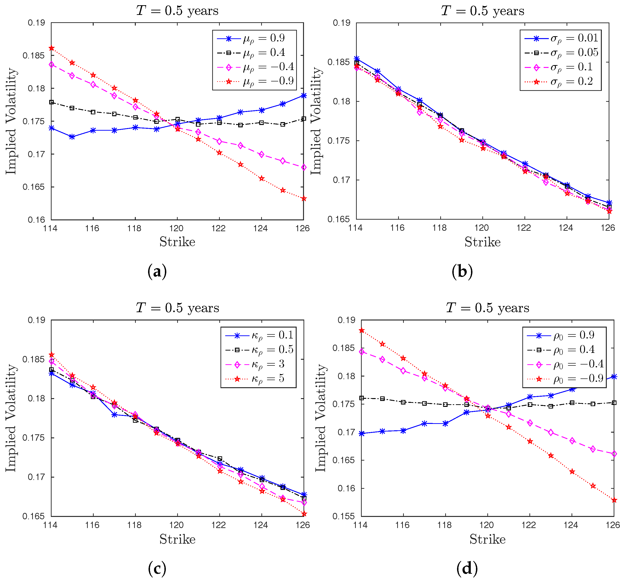
In this section, we analyze the effect of imposing stochastic correlation on the implied volatilities. To do this, we show the role of using stochastic correlation process in implied volatility, namely to see how the values of parameters of the correlation process will drive the implied volatilities. We display in Figure 1 the changes of implied volatilities by varying each parameter of stochastic correlation process. For this experiment, we prefer to use the HBM scheme.

We consider a Call-option with $S=120$, $T=0.5$ and the strikes from 114 to 126 in increments of 1, $r=1\%$. For the variance process, we set ${\nu }_0=0.03$, ${\mu }_{\nu }=0.04$, ${\kappa }_{\nu }=2.1,{\sigma }_{\nu }=0.4$, and, for the correlation process, we choose ${\kappa }_{\rho }=3.5$, ${\sigma }_{\rho }=0.1$, ${\mu }_{\rho }=-0.6$ (equal to the constant correlation) and set ${\rho }_0=-0.4$ except for the one that is varying. Finally, we set ${\rho }_2=0.1$ and use $M={10}^6$ for the Monte Carlo simulation.

From Figure 1, we realize that the parameters of correlation process can control the skewness or smiles of the implied volatilities. Compared to using a constant correlation parameter, including stochastic correlation provides more flexibility and can thus improve the calibration to the real market data.

4.3. A Comparison with the Effect of Stochastic Correlation

In order to be able to compare with the pure Heston price, in the numerical experiments above, we have initialized the stochastic correlation process such that it can rapidly reach its mean value. Now, we want to test our numerical schemes including the effect of stochastic correlations. Teng et al. (2016c) found the well approximated characteristic function of the Heston model extended by including stochastic correlations driven by the OU process in a closed-form, which can be used for analytical pricing purposes. Moreover, a comparison to the EM scheme has already been provided in Teng et al. (2016c); for more detailed information, we refer to Teng et al. (2016c).

Next, we test all of the numerical schemes by comparing them to the method in Teng et al. (2016c). For this, we take a five years Call with $S_0=100$ and report the price differences between using the proposed numerical schemes and the approach in Teng et al. (2016c) in

Table 6. Paramter values of the stochastic volatility and correlation: ${\kappa }_{\nu }=2.3,{\nu }_0={\mu }_{\nu }=0.04$, ${\sigma }_{\nu }=0.09$, ${\kappa }_{\rho }=2,{\rho }_0=-0.1,{\mu }_{\rho }=-0.5,{\sigma }_{\rho }=0.02,{\rho }_2=0,r=0$.

$\mathbf{\Delta }$	EM		HB	HBM
		$K=70$
1	$0.072\left(0.042\right)$		$-6.246\left(0.047\right)$	$-0.153\left(0.042\right)$
$1/2$	$-0.003\left(0.042\right)$		$-1.569\left(0.043\right)$	$0.007\left(0.042\right)$
$1/4$	$-0.089\left(0.042\right)$		$-0.339\left(0.042\right)$	$0.061\left(0.042\right)$
$1/8$	$0.013\left(0.042\right)$		$-0.071\left(0.042\right)$	$0.020\left(0.042\right)$
$1/16$	$0.033\left(0.042\right)$		$-0.014\left(0.042\right)$	$-0.000\left(0.042\right)$
$1/32$	$0.033\left(0.042\right)$		$-0.005\left(0.042\right)$	$-0.011\left(0.042\right)$
		$K=100$
1	$-0.006\left(0.033\right)$		$-4.924\left(0.039\right)$	$-0.182\left(0.033\right)$
$1/2$	$0.018\left(0.033\right)$		$-1.225\left(0.035\right)$	$-0.011\left(0.033\right)$
$1/4$	$-0.052\left(0.033\right)$		$-0.274\left(0.033\right)$	$0.027\left(0.033\right)$
$1/8$	$0.022\left(0.033\right)$		$-0.040\left(0.033\right)$	$0.021\left(0.033\right)$
$1/16$	$0.046\left(0.033\right)$		$-0.010\left(0.033\right)$	$-0.009\left(0.033\right)$
$1/32$	$0.047\left(0.033\right)$		$\left(0.033\right)$	$-0.011\left(0.033\right)$
		$K=140$
1	$-0.063\left(0.022\right)$		$-2.900\left(0.027\right)$	$-0.156\left(0.022\right)$
$1/2$	$-0.001\left(0.022\right)$		$-0.696\left(0.023\right)$	$-0.016\left(0.022\right)$
$1/4$	$-0.033\left(0.022\right)$		$-0.184\left(0.022\right)$	$-0.019\left(0.022\right)$
$1/8$	$-0.025\left(0.022\right)$		$-0.136\left(0.022\right)$	$-0.014\left(0.022\right)$
$1/16$	$-0.015\left(0.022\right)$		$-0.014\left(0.022\right)$	$-0.017\left(0.022\right)$
$1/32$	$0.031\left(0.022\right)$		$0.005\left(0.022\right)$	$-0.005\left(0.022\right)$

.

The used parameter values for $d{\nu }_t$ are not under the Feller condition. We thus obtain similar results to those of Case IV: the HB scheme does not perform well with a large time step $\mathsf{\Delta }$. From all the numerical experiments, we conclude that: the HB and HBM schemes outperform the EM scheme when the parameter values of $d\nu$ are not subject to the Feller condition. By contrast, under the Feller condition, the EM and HBM schemes are more favorable since they outperform the HB scheme at a large time step $\mathsf{\Delta }$.

5. Conclusions

In this work, we extended the Heston model by imposing stochastic correlations driven by a SDE. We have introduced different numerical algorithms including numerical analysis and compared their merits. We showed which algorithms are more favorable for which model parameterizations. Thereof, the HB and HBM scheme arose by adopting the QE scheme in Andersen (2008).

A couple of numerical results are provided. It has been shown that the numerical schemes proposed in this paper can work so well for the extended Heston by including stochastic correlations as the QE scheme in Andersen (2008) for the pure Heston model. Moreover, we realized the benefit of incorporating stochastic correlations by investigating the effect of stochastic correlations on the implied volatility. Because of the increased number of model parameters through the correlation process, the extended Heston with stochastic correlations can provide more than enough skews or smiles in the implied volatility as the market requires than the pure Heston model.

References

- Andersen, Leif. 2008. Simple and efficient simulation of the Heston stochastic volatility model. Journal of Computational Finance 11: 1–42. [Google Scholar] [CrossRef]
- Black, Fischer, and Myron Scholes. 1973. The Pricing of Options and Corporate Liabilities. Journal of Political Economy 81: 637–54. [Google Scholar] [CrossRef]
- Carr, Peter, and Dilip B. Madan. 1999. Option Valuation Using the Fast Fourier Transform. Journal of Computational Finance 2: 61–73. [Google Scholar] [CrossRef]
- Christoffersen, Peter, Steven Heston, and Kris Jacobs. 2009. The Shape and Term Structure of the Index Option Smirk: Why Multifactor Stochastic Volatility Models Work so Well. Management Science 55: 1914–32. [Google Scholar] [CrossRef]
- Elices, Alberto. 2009. Affine Concatenation. Wilmott Journal 1: 155–62. [Google Scholar]
- Euler, Leonhard. 1913. Institutiones Calculi Integralis. Berlin and Heidelberg: Springer, vol. 11. First published in 1768. Reprinted in Opera Omnia. [Google Scholar]
- Grzelak, Lech A., and Cornelis W. Oosterlee. 2011. On the Heston model with Stochastic Interest Rate. SIAM Journal on Financial Mathematics 2: 255–86. [Google Scholar] [CrossRef] [Green Version]
- Heston, Steven L. 1993. A Closed-Form Solution for options with Stochastic Volatility with Applications to Bond and Currency Options. The Review of Financial Studies 6: 327–43. [Google Scholar] [CrossRef]
- Kahl, Christian, and Peter Jäckel. 2005. Not-so-complex Logarithms in the Heston Model. Wilmott Magazine September: 94–103. [Google Scholar]
- Kloeden, Peter, and Eckhard Platen. 1999. Numerical Solution of Stochastic Differential Equations. New York: Springer-Verlag. [Google Scholar]
- Lee, Roger. 2004. Option pricing by transform methods: Extensions, unification, and error control. Journal of Computational Finance 7: 51–86. [Google Scholar] [CrossRef]
- Lewis, Alan L. 2001. Option Valuation under Stochastic Volatility. Newport Beach: Finance Press. [Google Scholar]
- Lipton, Alexander. 2002. The vol smile problem. Risk 8: 61–65. [Google Scholar]
- Ma, Jun. 2009. Pricing Foreign Equity Options with Stochastic Correlation and Volatility. Annals of Economics and Finance 2: 303–27. [Google Scholar]
- Maruyama, Gisiro. 1955. Continuous Markov processes and stochastic equations. Rendiconti del Circolo Matematico di Palermo 4: 48–90. [Google Scholar] [CrossRef]
- Mikhailov, Sergei, and Ullrich Nögel. 2003. Heston’s Stochastic Volatility Model: Implementation, Calibration and some Extensions. Wilmott Magazine July: 74–79. [Google Scholar]
- Milstein, Grigori Noichowitsch. 1974. Approximate integration of stochastic differential equations. Theory of Probability & Its Applications 19: 557–62. [Google Scholar]
- Teng, Long, Cathrin van Emmerich, Matthias Ehrhardt, and Michael Günther. 2014a. A Versatile Approach for Stochastic Correlation using Hyperbolic Functions. International Journal of Computer Mathematics 93: 524–39. [Google Scholar] [CrossRef]
- Teng, Long, Matthias Ehrhardt, and Michael Günther. 2014b. The pricing of Quanto options under dynamic correlation. Journal of Computational and Applied Mathematics 275: 304–10. [Google Scholar] [CrossRef]
- Teng, Long, Matthias Ehrhardt, and Michael Günther. 2016a. Modelling Stochastic Correlation. Journal of Mathematics in Industry 6: 1–18. [Google Scholar] [CrossRef]
- Teng, Long, Matthias Ehrhardt, and Michael Günther. 2016b. The Dynamic Correlation Model and its Application to the Heston model. In Innovations in Derivatives Markets. Edited by Kathrin Glau, Zorana Grbac, Matthias Scherer and Rudi Zagst. Munich: Technical University of Munich. [Google Scholar]
- Teng, Long, Matthias Ehrhardt, and Michael Günther. 2016c. On the Heston model with Stochastic Correlation. International Journal of Theoretical and Applied Finance 19: 1650033. [Google Scholar] [CrossRef]
- Uhlenbeck, George E., and Leonard S. Ornstein. 1930. On the Theory of Brownian Motion. Physical Review 36: 823–41. [Google Scholar] [CrossRef]
- Van Emmerich, Cathrin. 2006. Modelling Correlation as a Stochastic Process. Preprint 06/03. Wuppertal: University of Wuppertal. [Google Scholar]
Figure 1.
Comparison of implied volatilities for varying each parameter of stochastic correlation processes. (a) Varying ; (b) Varying ; (c) Varying ; (d) Varying .