Random Walker Coverage Analysis for Information Dissemination in Wireless Sensor Networks


Department of Informatics, Ionian University, 7 Tsirigoti Square, 49100 Corfu, Greece
*
Author to whom correspondence should be addressed.
Technologies 2017, 5(2), 33; https://doi.org/10.3390/technologies5020033
Submission received: 4 May 2017
/
Revised: 5 June 2017
/
Accepted: 7 June 2017
/
Published: 10 June 2017
(This article belongs to the Section Environmental Technology)
Abstract
:The increasing technological progress in electronics provides network nodes with new and enhanced capabilities that allow the revisit of the traditional information dissemination (and collection) problem. The probabilistic nature of information dissemination using random walkers is exploited here to deal with challenges imposed by unconventional modern environments. In such systems, node operation is not deterministic (e.g., does not depend only on network nodes’ battery), but it rather depends on the particulars of the ambient environment (e.g., in the case of energy harvesting: sunshine, wind). The mechanism of information dissemination using one random walker is studied and analyzed in this paper under a different and novel perspective. In particular, it takes into account the stochastic nature of random walks, enabling further understanding of network coverage. A novel and original analysis is presented, which reveals the evolution network coverage by a random walker with respect to time. The derived analytical results reveal certain additional interesting aspects regarding network coverage, thus shedding more light on the random walker mechanism. Further analytical results, regarding the walker’s spatial movement and its associated neighborhood, are also confirmed through experimentation. Finally, simulation results considering random geometric graph topologies, which are suitable for modeling mobile environments, support and confirm the analytical findings.
1. Introduction
During the last two decades, numerous wireless sensor networks (WSN) have been deployed for various activities [1,2,3,4,5,6]. Due to the continuous technological progress in electronics [7], reasonably inexpensive small nodes with high capabilities are now available [8,9]. In particular, the appearance on the market of small nodes with capabilities of energy harvesting (i.e., nodes capable of recharging their battery by acquiring energy from external sources) caused a revisit of fundamental networking problems (such as routing, medium access control, information dissemination, facility placement) from a new perspective [10,11,12].
WSN with energy-harvesting capabilities have lost their inherent deterministic reliability provided by batteries and need to operate in the uncertainty of the availability of natural resources. This trade-off of power over efficiency is more and more observed in technological advances; therefore there is a need for further investigation and reconsideration of traditional approaches in order to keep up with this progress. The stochastic nature of these modern networks challenges the application of the most widely-used methods for the dissemination (and similarly the collection) of information (e.g., flooding). New mechanisms have been developed and used for this purpose [13], one being the random walker [14,15,16,17].
Information propagation in various networks is crucial in order to perform a computational task, especially in the case of WSN where nodes are at a distance from each other, and therefore, they are obligated to communicate with one or more of the rest of the network nodes. Nowadays, technology has enabled the application of such devices in many fields. Taking into account the cost of energy and time for the proper operation of these networks, there is a strong need for efficient methods and approaches regarding the spread of information among the network’s nodes.
One of the known advantages of the random walker method is that during the process, it makes multiple revisits to the nodes at different times, until it fully covers the network. This fact increases the probability of a node to accept the visit of a random walker during the time period that it operates in active mode. In this study, the network topology is represented as random geometric graphs, since this graph category is considered suitable for modeling wireless sensor networks [18]. The topologies of geometric random graphs are also found in real-world systems, such as the thalamo-cortical system of the cat [19] and, in general, in the cortical system of living organisms [20,21].
In this work, the focus is on information dissemination using random walks. A random walker probabilistically chooses the next neighboring node to visit, independently of any previous visits. The probabilistic nature of this mechanism is suitable for dealing with the problem of nodes operating or not from time to time due to the energy availability. This mechanism is expected to probabilistically cover the whole network (i.e., reach all network nodes) using significantly less messages (one random walker movement corresponds to one message) in comparison to the use of deterministic flooding at the expense of increased termination time [22].
In the following sections, a novel analytical approach is proposed, showing how coverage is developed in relation to the number of random walker’s steps. First, the probability of a random walker approaching a node for the first time at each step is calculated. This probability is subsequently, used to calculate the number of nodes that had been visited by the random walker at least once, depending on the number of steps. The analytical results indicate that the evolution of the network coverage is independent of its density of connections. Only in marginally-sparse topologies, there is a significant time lag, as provided by the aforementioned analysis of this work. Extended simulations provide results that sufficiently support the analytical expectations.
Another contribution of this paper corresponds to additional results considering the walker’s spatial movement and its associated neighborhood, producing useful analytical results that subsequently enable the study of network coverage. These results are also validated through experimentation. Finally, the accordance between analytical and numerical results is shown by suitably illustrated results.
The structure of the rest of this paper is as follows: Section 2 briefly covers recent works related to information dissemination using random walkers. In Section 3, the evolution of coverage is analytically studied. This is the part of the paper that contains its main contribution. Section 4 includes the simulation outcomes that confirm the analytical results of the previous section, and finally, the conclusions are drawn in Section 5. There are also three appendices containing the detailed proofs for the corresponding theorems and corollaries that lie within the main text.
2. Related Work
The choice of the model of a geometric random graph to represent WSN and ad hoc networks is quite common in the literature, e.g., [16,23,24,25,26,27,28,29]. One of the most most comprehensive studies on geometric random graphs can be found in [18] by Penrose. In addition, in [30], there is a thorough study on geometric graphs with analytic results (studying graphs of higher dimensions, as well). In this work, Dall and Christensen investigate mainly the radius threshold to achieve critical connectivity.
The throughput of a mobile ad hoc network powered by energy harvesting is studied and analyzed by Huang [31], using a stochastic, geometric approach. Regarding information dissemination, probabilistic flooding is a popular approach (see for example [32,33,34,35]). Random walkers have been extensively examined in the literature. In particular, in [14], a mathematical framework for random walks on temporal networks is presented by Hoffmann et al. using an approach that provides a compromise between abstract, but unrealistic models and data-driven, but non-mathematical approaches.
Starnini et al. [15] describe a study on how random walks unfold on temporally-evolving networks with the use of empirical dynamical networks of contacts between individuals. Tzevelekas et al. in [16] present the same problem addressed in this work with the technique of a random walker with jumps. Oikonomou et al. in [25] investigate the use of multiple random walkers and related replication mechanisms.
Recently, Jamoos in [36] studied some network properties of WSNs, proposing an improved decision fusion model in order to optimize the energy and bandwidth consumption. Broutin et al. [37] explore random geometric graphs and the associated problem of connectivity. In particular, they use the so-called random geometric “irrigation” graphs, and then, they provide insightful results on the density of these graphs for a chosen radius. Mao in [38] discusses the behavior of the phase transition of connectivity for geometric random graphs.
Random hypergraphs are considered by Lunagómez et al. [39], especially their geometric representations. The authors are concentrated on the probability distribution and its effect on the network topology (and therefore, its properties). Recently, Kalhe in [40] revisits reviewed related literature on random geometric graphs with a focus on random simplicial complexes. In one of the most recent works related to random walkers on graphs, Estrada et al. [41] describe a random walker model where the agent is able to perform long-range hops. This extension seems to reduce the hitting time in comparison to the standard walker.
Lima and Barros [29] present an algorithm that improves the data-gathering performance by generating constrained random walks. Zuniga et al. [17] study non-revisiting random walks. The work of Mabrouki et al. [42] provides an analytical model to evaluate the performance of a random walk-based routing protocol for wireless sensor networks with special attention to two metrics: the mean system data gathering delay and the induced spatial distribution of energy consumption.
A forwarding protocol based on biased random walks is proposed combined with a lukewarm potato forwarding protocol that uses local information about neighbors, and their next active period to make forwarding decisions is presented by Beraldi et al. [24]. A routing protocol based on a random walk is proposed by Tian et al. [43] that achieves load balancing without requiring global location information. Boyd et al. [23] present a theoretical approach of random walkers in geometric random graphs that are developed in a d-dimensional torus.
These works, however, do not take into account network coverage as the evolution of time, apart from some special topologies (e.g., fully-connected networks considered in [25]). The work in [12] by Huang and Tseng discuss thoroughly the sensing ranges of sensors in wireless sensor networks. A similar work to this one is described by Mian et al. [44], where the authors propose the so-called “attenuation” metric that shows the speed of the random walker’s movement. Cover time is examined by Avin and Ercal [45]. There are interesting theoretical results regarding the achieved optimal cover time with high probability, providing tight lower bounds from the chosen radius of the geometric graphs.
The study of the network coverage achieved by a random walker acting on it constitutes the main contribution of this work. Previous works had shown an analytical expression only for fully-connected networks [25]. In this paper, an analytic solution is presented in response to the problem of network coverage achieved by a random walker, which applies to any connected network regardless of the density of its connections. The results presented in this work are in accordance with the former in the special case of the fully-connected network.
3. Analysis
In this work, the mechanism of the random walker was selected in order to study the information dissemination. A random walker can be seen as an entity, beginning at the initiator node, that chooses randomly (uniformly) to visit a one-hop neighbor of the node where it currently resides. Then, this “agent” continues in a similar manner until the entire network is covered (i.e., all nodes are visited by the walker).
In order to analytically model network coverage when a random walker is employed, the following assumptions take place. The network nodes are uniformly distributed on a plain area sized , that is a unit square. All considered networks are connected (a network is connected when there is a path between every pair of nodes). Each node of the network has the same transmission range .
The following notation is also used: N denotes the number of nodes on each network, and is a stochastic variable representing the number of nodes who have received at least one visit after t random walker’s steps. Each node has transmission range . Hence, the surface covered by its transmissions is (ideally) . Throughout this work, this surface is referred to as the node’s radius.
Given that nodes are uniformly distributed, the number of network nodes located in an area of region is (on average) . Thus, each network node will have on average neighbors. The random walker’s spatial movement (i.e., the euclidean distance covered) on each step is on average (the proof is in Appendix A). This result is also confirmed later through simulations.
The mean spatial movement of a random walker from a position after t steps is given by , where l is the Euclidean distance covered in each step [46]. Thus, using the average random walker’s spatial movement on each step mentioned in the previous paragraphs, it holds that and, consequently,
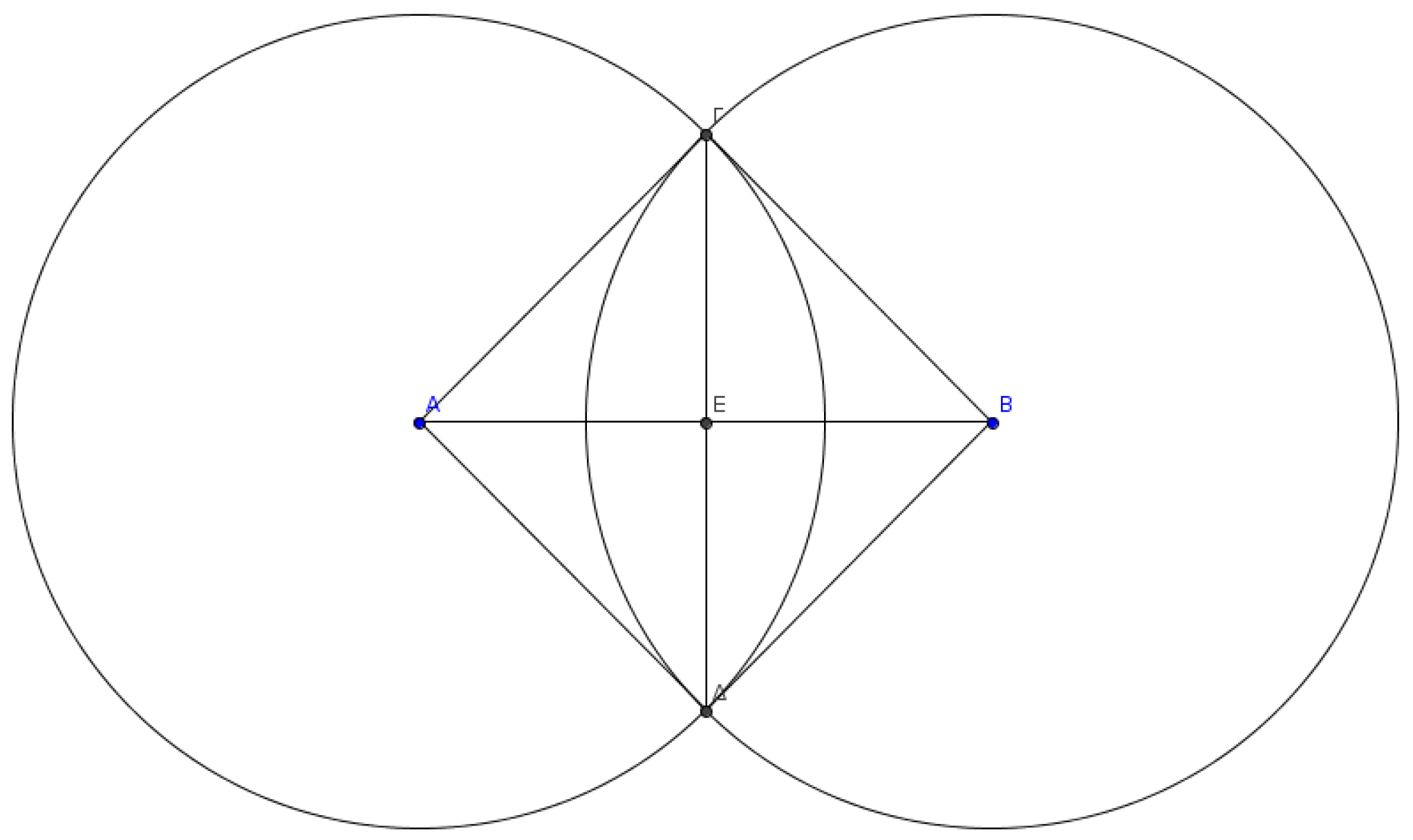
From the above Equation (1), it follows that when t ≤ 9, then < 2 . Therefore, the neighborhood of the node visited by the random walker before t ≤ 9 steps and the neighborhood of the node on which it lies now will overlap, and nodes on the corresponding overlapping surface are neighbors of both (see Figure 1). The number of those nodes is analogous on average to the overlapping surface. The area of this surface is given by the following theorem:
Theorem 1.
On a random walker acting on a geometric random graph, the neighborhood of the node visited by the random walker before t time steps (where ) and the neighborhood of the node on which it lies now have an overlapping surface :
The proof of Theorem 1 is in Appendix B.
In brief, Equation (2) is used to calculate the common neighborhood of the currently visited node with the previously visited ones, choosing at each time step the node that corresponds to the value of t (i.e., for the node visited one time step before, for the node visited two time steps before, and so on).
On this basis, each time the random walker chooses the next step node from the current set of neighbor nodes, i.e., nodes at . Note that the random walker has already visited at least one of these nodes, in particular the previous node, which the random walker visited one time step before. The probability for the node that the random walker visited before t (where ) steps to belong to this set is proportional to the fraction of the area of the overlapping surface to the node’s neighborhood surface (see Figure 1).
Let V indicate the number of neighboring nodes that have already been visited by the random walker.
Corollary 1.
The expected value of V is approximately equal to 2.838.
The proof is in Appendix C.
Given the analysis so far, it is evident that the number of neighbors not visited in the first nine steps is . This also holds when applied for any arbitrary starting point (i.e., ) of the random walker and not necessarily for . Simulation results presented later support this claim. Therefore, the probability for the random walker to select a node that has not been visited during the last nine steps is given by the following equation:
Equation (3) is the basis to calculate . In particular, the number of network nodes that have received at least one random walker visit after t steps is equal to the number of nodes that have been visited on the previous step, i.e., plus the probability that the next node to be visited has not been visited before. As shown in Appendix D, the analytical expression of is given by Equation (4):
The following corollary expresses as a discrete function of the time step t with parameters the transmission range and the number of nodes N.
Corollary 2.
Network coverage is given by:
The proof can be found in Appendix D.
The ratio of the network nodes that have been visited so far by the random walker over the total number of network nodes after every time step is calculated using Equation (5).
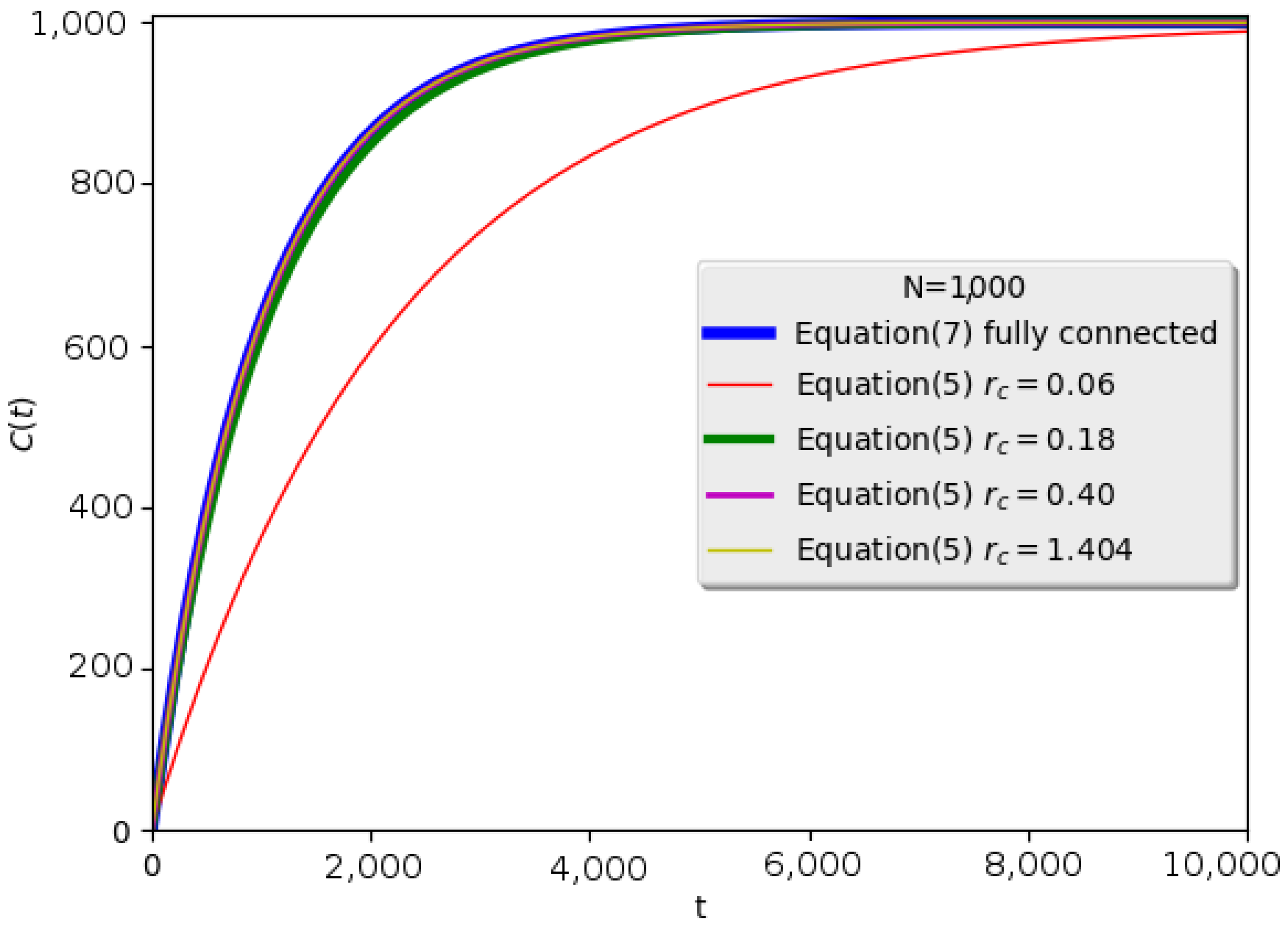
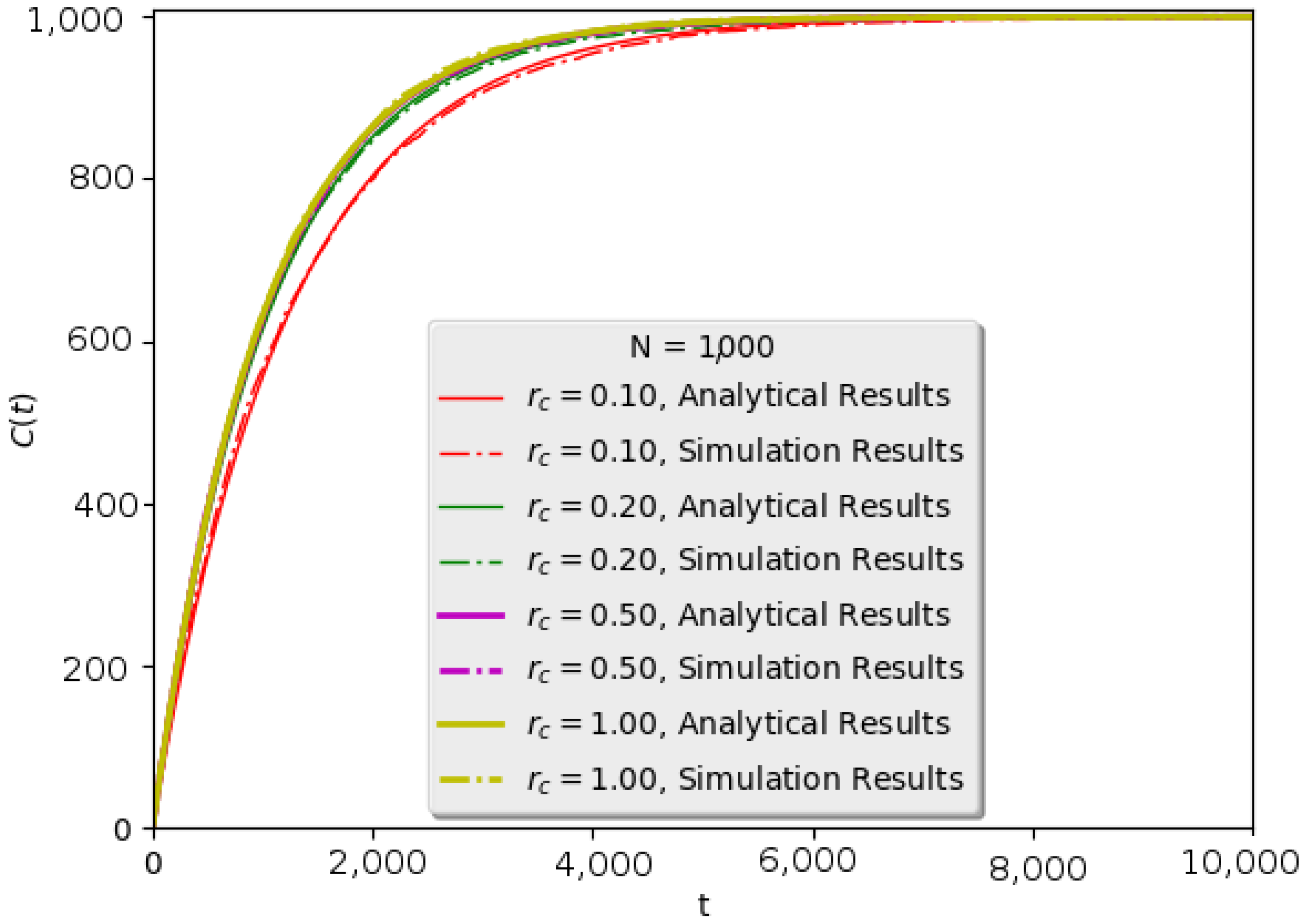
Figure 2 depicts the evolution of for a geometric random graph network of and various values of . For , the network is marginally connected (i.e., the smallest value of for which all nodes belong to the network with high probability) with the average number of links per node being ; thus, the curve is the lowest one (depicted with the red color). This is explained since in Equation (4) is much smaller than one. In all other cases where the average number of links per node is much greater (100, 500 and 1000), , and the relevant curves are close to the results presented in [25] i.e., Equation (7).
Equation (7) refers to a fully-connected network.
The proof for this theorem can be found in Appendix E.
Given Equation (5), it is observed that network coverage evolves almost independently of the network’s density of connections, since the square of the radius is taken into account, which also lies in the denominator of the fraction. Only on marginally sparse networks, there is a distinct time lag, since in this case, the value of is the minimum one. The analysis in this section resulted in Equations (5) and (6), which demonstrate the evolution of the network coverage using a random walker in relation to time (a walker’s step corresponds to a single time unit). These results are experimentally examined in the next section.
4. Simulation Results
In this section, indicative simulations are provided in order to validate the analytical results and confirm the applicability of the proposed modeling. The following simulations were made on a custom-made simulator. The simulator was developed in Python 3.0, using the SciPy and NumPy libraries, whereas the graphs were plotted using the Matplotlib library. Randomness was generated using the random number generator of Scipy (i.e., the Mersenne Twister pseudo-random number generator) with a different seed each time.
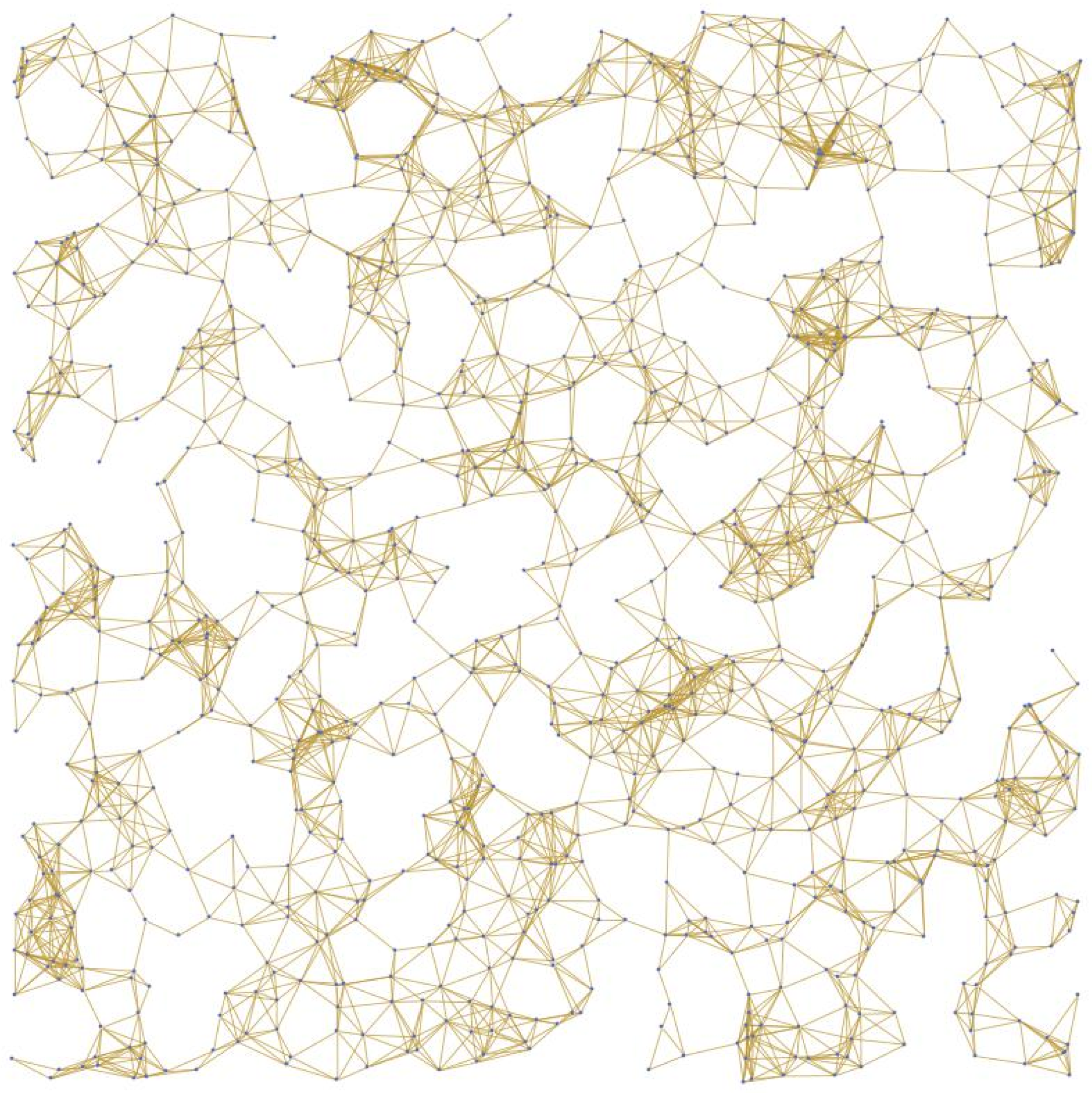
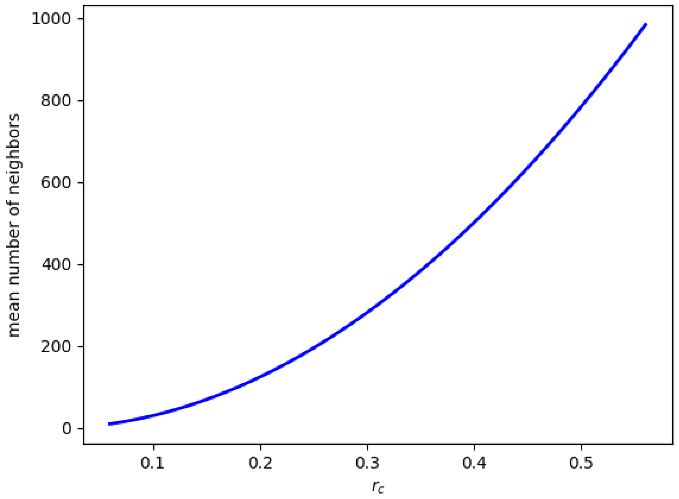
Simulations are performed on random geometric networks with 1000 and 10,000 nodes (see Figure 3 for an indicative snapshot of a marginally-connected network). The geometric area chosen for the development of the networks is the 2D-torus as suggested by the literature (e.g., in [23]). The networks assumed for simulation purposes are from marginally- to fully-connected (therefore, there are various values for the radius ), and on each of them, a random walker is employed. Furthermore, in Figure 4, the mean number of neighbors for a network of 1000 nodes is depicted as a function of . It is obvious that for each node, the longer the radius was, the more (on average) neighbors it had.
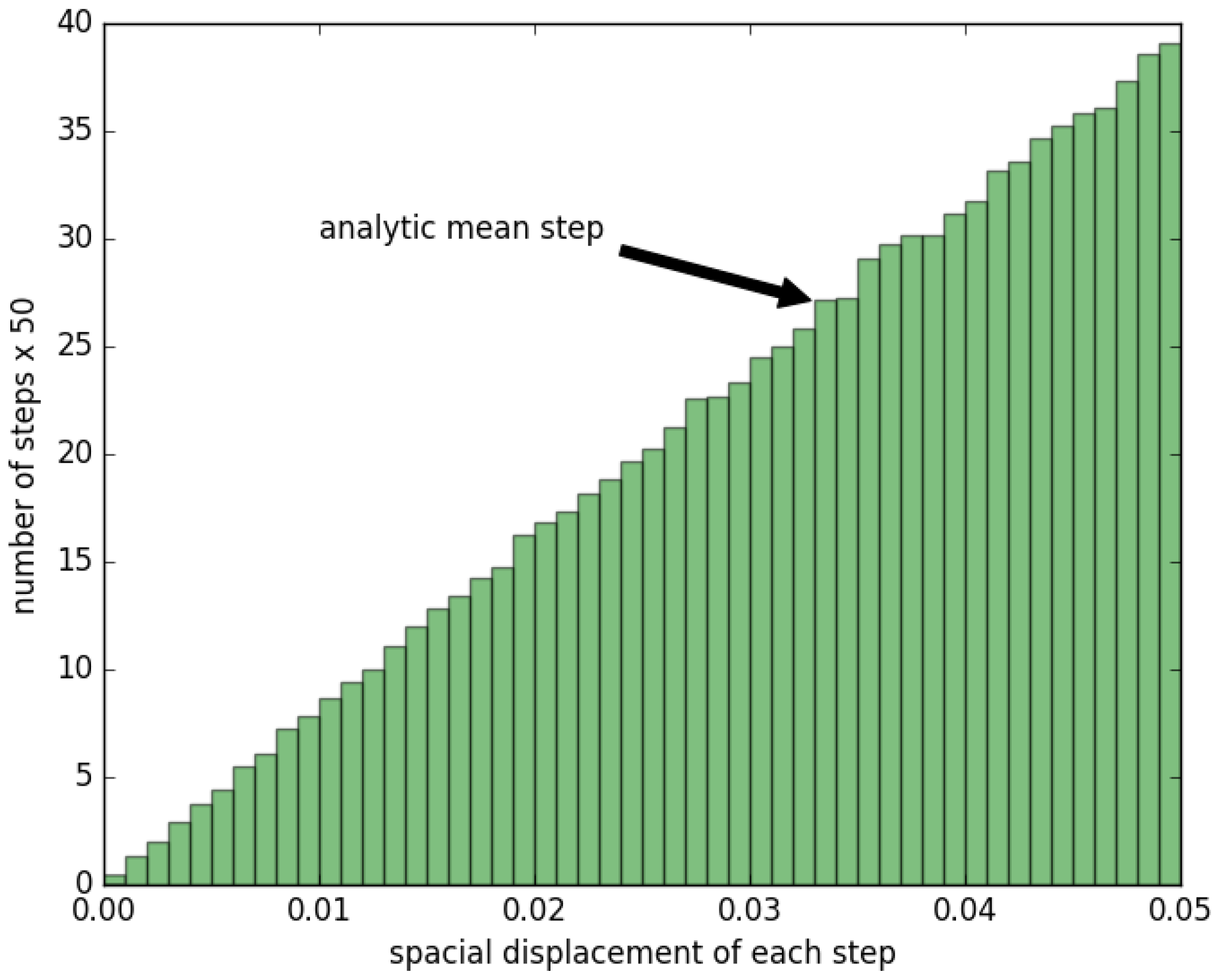
To begin with, the average spatial movement of the random walker is tested on each step. This is described by the following equation:
where is the average distance covered by the random walker.
The obtained simulation results of a random walker doing steps on a network with nodes and are shown in Figure 5, and as depicted, they are in accordance with Equation (8). In particular, the equation’s result is 0.033, whereas the one derived from the simulation is 0.033.
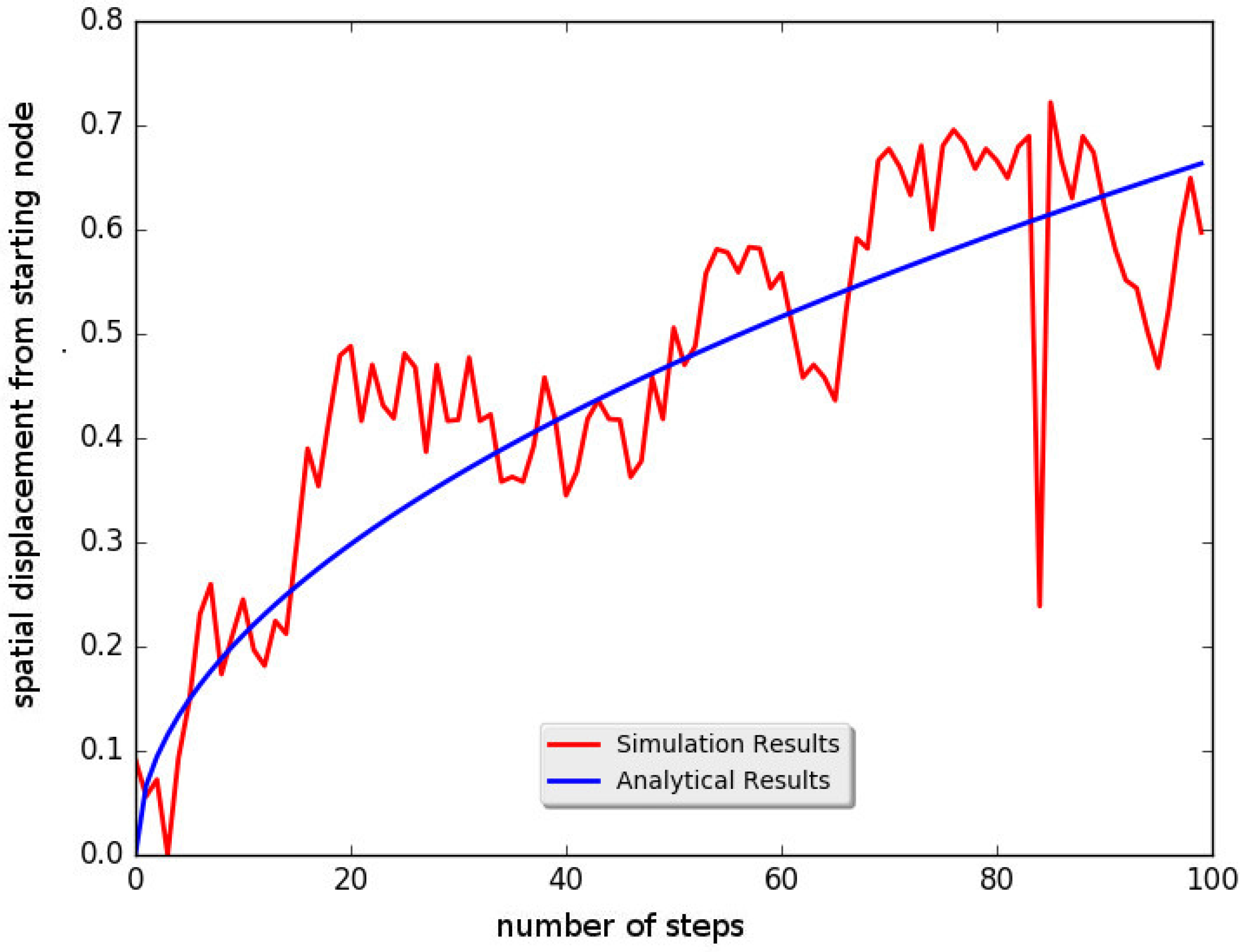
Afterwards, Equation (1) is evaluated considering a network with 1000 nodes and radius . For this network, a random walker performed 100 steps, and on each step, the spatial displacement starting from the starting node is computed. The results are illustrated in Figure 6 along with the analytic results of Equation (1). From the depicted comparison, it seems that the analytical result comprehends the actual walker’s movement. Both curves are incremental in a similar manner, and although there are some spikes on the simulation curve, Equation (1) successfully describes the underlying behavior.
In order to evaluate Equation (3), the number of each node’s neighbors that were visited by the random walker in the last nine steps is monitored for multiple simulations. The simulations took place in 10 networks of nodes with the random walker performing steps for each one of them. The results confirmed the relevant analytical results (analytic calculation = 2.838, simulation results’ mean = 3.264, std = 1.718).
In the sequel, simulations are performed on networks with nodes and varied transmission range and in order to verify the main arguments of this work. For each value of , 10 networks are created, and on each one of them, a random walker runs for steps. On the corresponding illustrations the number of nodes that had received at least one random walker’s visit (i.e., ) is given on the vertical axis, while the number of random walker’s steps (t) lies on the horizontal.
Simulation results for 100 networks with and the mean number of direct neighbors = 12 are presented in Figure 7. On the other hand, in Figure 8, results are depicted for networks with radius and mean number of direct neighbors = 35, 158, 834, 997, respectively. In Figure 8, it is shown that the coverage of the network is independent of the density of the connections.
From the aforementioned results and the associated figures, it seems that the previously stated arguments regarding the network coverage in geometric random graphs through the random walker mechanism are confirmed. Therefore, these simulation results are fully consistent with the analytical expectations presented in this work.
Geometric Networks on a Grid
In order to test the proposed analysis in extreme conditions, simulations are also conducted on grid geometric networks. A grid geometric network is composed of nodes deployed on a 2D torus grid. In particular, each node is located on the intersection of the grid in a 2D-torus surface. All considered networks are connected with nodes each and varied transmission range. Simulation results are presented in Figure 9 and Figure 10.
As can be observed, even in these conditions, where the randomness of the network is repealed in the simulation, the results fully support the analytical model proposed in the main part of this work. Although this model was based on the random walker mechanism acting on randomly-generated graphs, the results of Figure 9 and Figure 10 showed that it is able to describe a deterministic variant, as well.
5. Conclusions
The random walker’s mechanism is used for information dissemination in order to exploit the probabilistic advantage in the emerging new network environment like energy-harvesting networks. In such environments, approaches like flooding are not suitable since nodes may stop operating from time to time due to energy unavailability resulting in temporarily disconnected networks. In such systems with stochastic behavior, the use of a random walker for the dissemination of information can be quite useful, reducing the number of messages among the nodes. Nevertheless, there is disadvantage with respect to the increased time required for the coverage of the network.
In this work, a handy analytical tool is given that enables the study of the coverage of a network by a random walker over time. The paper focuses on the study of network coverage achieved by a random walker acting on it, under a novel and original perspective. As the random walker acts on a given network, it inevitably revisits the network’s nodes due to the probabilistic nature of the random walker movement. This fact enables the overcoming of the problem of the unavailability of certain nodes from time to time because of a temporary lack of energy. The random walker probabilistically chooses the next neighboring node to visit, without considering any previous visits.
To sum up the contribution of this study, a novel analytical approach is described, presenting the coverage rate in relation to the number of random walker’s steps. In this direction, the probability for the random walker to reach a node for the first time at each step is calculated. Then, this probability value is used to find the number of nodes that had been visited by the random walker, which depends on the number of steps. There are also detailed results on the neighborhood surface in a random geometric graph, as well as some formulas on the average movement of the walker.
This analysis led to the conclusion that the coverage is independent of the network’s connection density (significant time lag is met only in marginally sparse topologies). The analytical findings presented in this work were also evaluated through simulation results in order to be properly verified. As was shown through indicative examples and figures, the presented analytical results were in accordance with the simulation outcomes, even for grid topologies.
Finally, the results of this work could trigger further investigation of the random walker mechanism in geometric graphs, under different assumptions and functionality modes. For example, one could consider the analytical version of the coverage when multiple walkers are employed, or when each node is weighted according to some metric, e.g., its “popularity” (i.e., the number of neighbors); for example, to investigate how the coverage would be affected if a two-hop distance estimation [47] is considered.
Author Contributions
All of the authors have contributed extensively to this study. Konstantinos Skiadopoulos and Konstantinos Oikonomou conceived of the initial idea. They both developed the initial formulation described in the main part. Konstantinos Skiadopoulos and Konstantinos Giannakis thoroughly analyzed the current literature, and they compared it with the described approach. Konstantinos Oikonomou was responsible for supervising the progress and the finishing of this work. Konstantinos Skiadopoulos and Konstantinos Oikonomou contributed to the proper typing of formal definitions and the math used in the paper. Konstantinos Skiadopoulos and Konstantinos Giannakis collaborated in the production of the experimental results. All of the authors contributed to the writing of the paper. All authors have read and approved the final manuscript.
Conflicts of Interest
The authors declare no conflict of interest.
Appendix A. Random Walker’s Spatial Displacement after One Step
The network nodes are uniformly distributed on the field, so the average spatial displacement of a random walker after every step is equal to the average distance of any point of a circle from the center. To calculate the average distance of a point from the center of the circle of radius R to which it belongs, the following distribution function is used.
This distribution function weights each radius r according to the circumference of a very thin annulus with that radius. To calculate the mean value of distance from the center of the circle, the following formula is used:
Appendix B. Overlapping Surface
Let B be the random walker’s current position and A a previous position t steps before, where (Figure A1). Distance is on average: (Equation (1)). Furthermore, .
Figure A1.
B current position of random walker and A random walker’s position before t steps.
From the Pythagorean theorem, it holds that: . Moreover, for the following angles it holds that .
The area of the meniscus constituting the common surface of the two circles is given by the following formula, where: is the surface of the circular sector and is the triangle’s area.
Consequently, two nodes t steps () apart on the random walker’s path have on average an area of as a common neighborhood surface.
Appendix C. Proof of Corollary 1
The analysis presented in Section 3 concluded that the number of nodes that has been already visited by the random walker on the last nine steps and that belong to the set of the neighbors of the node on which it is located is:
Appendix D. The Analytical Expression of C(t)
Using from Equation (3), the following recursive form of is produced.
The solution of the simple first order difference equation for is:
Appendix E. Equivalence of Equations (5) and (7)
If is so large that the network topology becomes the complete graph, i.e., the number of neighbor nodes , the , assuming large N, then Equation (5) becomes:
Because:
and if:
In Equation (A8), if: is replaced by: ():
In order to prove that Equation (A11) is equivalent to Equation (7), it is sufficient to show that: and: are equal. If they are equal:
therefore, if and are equal, the following should be true.
but:
and:
References
- Anastasi, G.; Farruggia, O.; Re, G.L.; Ortolani, M. Monitoring High-Quality Wine Production using Wireless Sensor Networks. In Proceedings of the 2009 42nd Hawaii International Conference on System Sciences, Big Island, HI, USA, 5–8 January 2009; pp. 1–7. [Google Scholar]
- Catania, P.; Vallone, M.; Re, G.L.; Ortolani, M. A wireless sensor network for vineyard management in Sicily (Italy). Agric. Eng. Int. CIGR J. 2013, 15, 139–146. [Google Scholar]
- Anastasi, G.; Re, G.L.; Ortolani, M. WSNs for structural health monitoring of historical buildings. In Proceedings of the 2009 IEEE 2nd Conference on Human System Interactions, (HSI’09), Catania, Italy, 21–23 May 2009; pp. 574–579. [Google Scholar]
- Peiris, V. Highly Integrated Wireless Sensing for Body Area Network Applications. 2013. Available online: http://spie.org/newsroom/5120-highly-integrated-wireless-sensing-for-body-area-network-applications (accessed on 25 August 2016).
- Hart, J.K.; Martinez, K. Environmental Sensor Networks: A revolution in the earth system science? Earth Sci. Rev. 2006, 78, 177–191. [Google Scholar] [CrossRef]
- Huang, X.; Yi, J.; Chen, S.; Zhu, X. A Wireless Sensor Network-Based Approach with Decision Support for Monitoring Lake Water Quality. Sensors 2015, 15, 29273–29296. [Google Scholar] [CrossRef] [PubMed]
- Gungor, V.C.; Hancke, G.P. Industrial wireless sensor networks: Challenges, design principles, and technical approaches. IEEE Trans. Ind. Electron. 2009, 56, 4258–4265. [Google Scholar] [CrossRef]
- Akyildiz, I.; Vuran, M. Wireless Sensor Networks (Advanced Texts in Communications and Networking); Wiley: New York, NY, USA, 2010. [Google Scholar]
- Akyildiz, I.F.; Su, W.; Sankarasubramaniam, Y.; Cayirci, E. Wireless Sensor Networks: A Survey. Comput. Netw. 2002, 38, 393–422. [Google Scholar] [CrossRef]
- Gong, P.; Xu, Q.; Chen, T.M. Energy Harvesting Aware routing protocol for wireless sensor networks. In Proceedings of the 2014 9th International Symposium on Communication Systems, Networks and Digital Signal Processing (CSNDSP), Manchester, UK, 23–25 July 2014. [Google Scholar]
- Yick, J.; Mukherjee, B.; Ghosal, D. Wireless sensor network survey. Comput. Netw. 2008, 52, 2292–2330. [Google Scholar] [CrossRef]
- Huang, C.F.; Tseng, Y.C. The coverage problem in a wireless sensor network. Mob. Netw. Appl. 2005, 10, 519–528. [Google Scholar] [CrossRef]
- Nakamura, E.F.; Loureiro, A.A.F.; Frery, A.C. Information Fusion for Wireless Sensor Networks: Methods, Models, and Classifications. ACM Comput. Surv. 2007, 39. [Google Scholar] [CrossRef]
- Hoffmann, T.; Porter, M.A.; Lambiotte, R. RandomWalks on Stochastic Temporal Networks. In Temporal Networks; Holme, P., Saramäki, J., Eds.; Springer: Berlin/Heidelberg, Germany, 2013; pp. 295–313. [Google Scholar]
- Starnini, M.; Baronchelli, A.; Barrat, A.; Pastor-Satorras, R. Random walks on temporal networks. Phys. Rev. E 2012, 85, 056115. [Google Scholar] [CrossRef] [PubMed]
- Tzevelekas, L.; Oikonomou, K.; Stavrakakis, I. Random walk with jumps in large-scale random geometric graphs. Comput. Commun. 2010, 33, 1505–1514. [Google Scholar] [CrossRef]
- Zuniga, M.; Avin, C.; Hauswirth, M. Querying Dynamic Wireless Sensor Networks with Non-revisiting Random Walks. In Proceedings of the 7th European Conference on Wireless Sensor Networks (EWSN 2010), Coimbra, Portugal, 17–19 February 2010; Silva, J.S., Krishnamachari, B., Boavida, F., Eds.; Springer: Berlin/Heidelberg, Germany, 2010. [Google Scholar]
- Penrose, M.D. Random Geometric Graphs; Oxford Studies in Probability; Oxford University Press: Oxford, UK, 2004. [Google Scholar]
- Costa, L.D.F.; Batista, J.L.; Ascoli, G.A. Communication Structure of Cortical Networks. Front. Comput. Neurosci. 2011, 5, 6. [Google Scholar] [CrossRef] [PubMed]
- Kaiser, M.; Martin, R.; Andras, P.; Young, M.P. Simulation of robustness against lesions of cortical networks. Eur. J. Neurosci. 2007, 25, 3185–3192. [Google Scholar] [CrossRef] [PubMed]
- Newman, M.E. The structure and function of complex networks. SIAM Rev. 2003, 45, 167–256. [Google Scholar] [CrossRef]
- Gkantsidis, C.; Mihail, M.; Saberi, A. Random walks in peer-to-peer networks. In Proceedings of the Twenty-Third AnnualJoint Conference of the IEEE Computer and Communications Societies, (INFOCOM 2004), Hong Kong, China, 7–11 March 2004; Volume 1. [Google Scholar]
- Boyd, S.; Ghosh, A.; Prabhakar, B.; Shah, D. Mixing times for random walks on geometric random graphs. In Proceedings of the SIAM Workshop on Analytic Algorithmics and Combinatorics (ANALCO), Vancouver, BC, Canada, 22 January 2005; pp. 240–249. [Google Scholar]
- Beraldi, R.; Baldoni, R.; Prakash, R. A biased random walk routing protocol for wireless sensor networks: The lukewarm potato protocol. IEEE Trans. Mob. Comput. 2010, 9, 1649–1661. [Google Scholar] [CrossRef]
- Oikonomou, K.; Kogias, D.; Stavrakakis, I. A Study of Information Dissemination Under Multiple Random Walkers and Replication Mechanisms. In Proceedings of the Second International Workshop on Mobile Opportunistic Networking, (MobiOpp’10), Pisa, Italy, 22–23 February 2010; ACM: New York, NY, USA, 2010; pp. 118–125. [Google Scholar]
- Kenniche, H.; Ravelomananana, V. Random geometric graphs as model of wireless sensor networks. In Proceedings of the 2nd International Conference on Computer and Automation Engineering (ICCAE), Singapore, 26–28 February 2010. [Google Scholar]
- Ren, Y.; Qin, Y.; Wang, B.; Zhang, H.; Zhang, S. A random geometric graph coverage model of wireless sensor networks. In Proceedings of the 2006 IET International Conference on Wireless, Mobile and Multimedia Networks, Hangzhou, China, 6–9 November 2006. [Google Scholar]
- Karamchandani, N.; Manjunath, D.; Yogeshwaran, D.; Iyer, S.K. Evolving Random Geometric Graph Models for Mobile Wireless Networks. In Proceedings of the 4th International Symposium on Modeling and Optimization in Mobile, Ad Hoc and Wireless Networks, Boston, MA, USA, 26 February–2 March 2006. [Google Scholar]
- Lima, L.; Barros, J. Random Walks on Sensor Networks. In Proceedings of the 2007 5th International Symposium on Modeling and Optimization in Mobile, Ad Hoc and Wireless Networks and Workshops, Limasso, Cyprus, 16–20 April 2007; pp. 1–5. [Google Scholar]
- Dall, J.; Christensen, M. Random geometric graphs. Phys. Rev. E 2002, 66, 016121. [Google Scholar] [CrossRef] [PubMed]
- Huang, K. Throughput of wireless networks powered by energy harvesting. In Proceedings of the 2011 Conference Record of the Forty Fifth Asilomar Conference on Signals, Systems and Computers (ASILOMAR), Pacific Grove, CA, USA, 6–9 November 2011; pp. 8–12. [Google Scholar]
- Oikonomou, K.; Kogias, D.; Stavrakakis, I. Probabilistic Flooding for Efficient Information Dissemination in Random Graph Topologies. Comput. Netw. 2010, 54, 1615–1629. [Google Scholar] [CrossRef]
- Stauffer, A.O.; Barbosa, V.C. Probabilistic heuristics for disseminating information in networks. IEEE ACM Trans. Netw. 2007, 15, 425–435. [Google Scholar] [CrossRef]
- Crisóstomo, S.; Schilcher, U.; Bettstetter, C.; Barros, J. Analysis of probabilistic flooding: How do we choose the right coin? In Proceedings of the 2009 IEEE International Conference on Communications (ICC’09), Dresden, Germany, 14–18 June 2009; pp. 1–6. [Google Scholar]
- Gaeta, R. Generalized Probabilistic Flooding in Unstructured Peer-to-Peer Networks. IEEE Trans. Parallel Distrib. Syst. 2011, 22, 2055–2062. [Google Scholar] [CrossRef]
- Jamoos, A. Improved Decision Fusion Model for Wireless Sensor Networks over Rayleigh Fading Channels. Technologies 2017, 5, 19. [Google Scholar] [CrossRef]
- Broutin, N.; Devroye, L.; Lugosi, G. Almost optimal sparsification of random geometric graphs. Ann. Appl. Probab. 2016, 26, 3078–3109. [Google Scholar] [CrossRef]
- Mao, G. Phase Transitions in Large Networks. In Connectivity of Communication Networks; Springer: Cham, Switzerland, 2017; pp. 149–174. [Google Scholar]
- Lunagómez, S.; Mukherjee, S.; Wolpert, R.L.; Airoldi, E.M. Geometric representations of random hypergraphs. J. Am. Stat. Assoc. 2016, 363–383. [Google Scholar] [CrossRef]
- Kahle, M. Topology of random simplicial complexes: A survey. AMS Contemp. Math. 2014, 620, 201–222. [Google Scholar]
- Estrada, E.; Delvenne, J.C.; Hatano, N.; Mateos, J.L.; Metzler, R.; Riascos, A.P.; Schaub, M.T. Random Multi-Hopper Model. Super-Fast Random Walks on Graphs. arXiv 2016. [Google Scholar]
- Mabrouki, I.; Lagrange, X.; Froc, G. Random Walk Based Routing Protocol for Wireless Sensor Networks. In Proceedings of the 2nd International Conference on Performance Evaluation Methodolgies and Tools, (ValueTools ’07), Nantes, France, 22–27 October 2007; ICST (Institute for Computer Sciences, Social-Informatics and Telecommunications Engineering): Brussels, Belgium, 2007; pp. 71:1–71:10. [Google Scholar]
- Tian, H.; Shen, H.; Matsuzawa, T. Random Walk Routing in WSNs with Regular Topologies. J. Comput. Sci. Technol. 2006, 21, 496–502. [Google Scholar] [CrossRef]
- Mian, A.N.; Beraldi, R.; Baldoni, R. On the coverage process of random walk in wireless ad hoc and sensor networks. In Proceedings of the 2010 IEEE 7th International Conference on Mobile Adhoc and Sensor Systems (MASS), San Francisco, CA, USA, 8–12 November 2010; pp. 146–155. [Google Scholar]
- Avin, C.; Ercal, G. On the cover time of random geometric graphs. In Proceedings of the International Colloquium on Automata, Languages, and Programming, Lisbon, Portugal, 11–15 July 2005; Springer: Berlin/Heidelberg, Germany, 2005; pp. 677–689. [Google Scholar]
- Weisstein, E.W. A Wolfram Web Resource: Random Walk–2-Dimensional. Available online: http://mathworld.wolfram.com/RandomWalk2-Dimensional.html (accessed on 8 April 2016).
- Kim, S.; Park, S.Y.; Kwon, D.; Ham, J.; Ko, Y.B.; Lim, H. Two-hop distance estimation in wireless sensor networks. Int. J. Distrib. Sens. Netw. 2017, 13. [Google Scholar] [CrossRef]
Figure 1.
Common neighborhood surfaces of nodes sequentially visited by the random walker. Eventually, the random walker’s steps are not straight as in the figure; the Euclidean distance from the original node A is given by Equation (1). The colored gray area is still the overlapping surface for .
Figure 1.
Common neighborhood surfaces of nodes sequentially visited by the random walker. Eventually, the random walker’s steps are not straight as in the figure; the Euclidean distance from the original node A is given by Equation (1). The colored gray area is still the overlapping surface for .
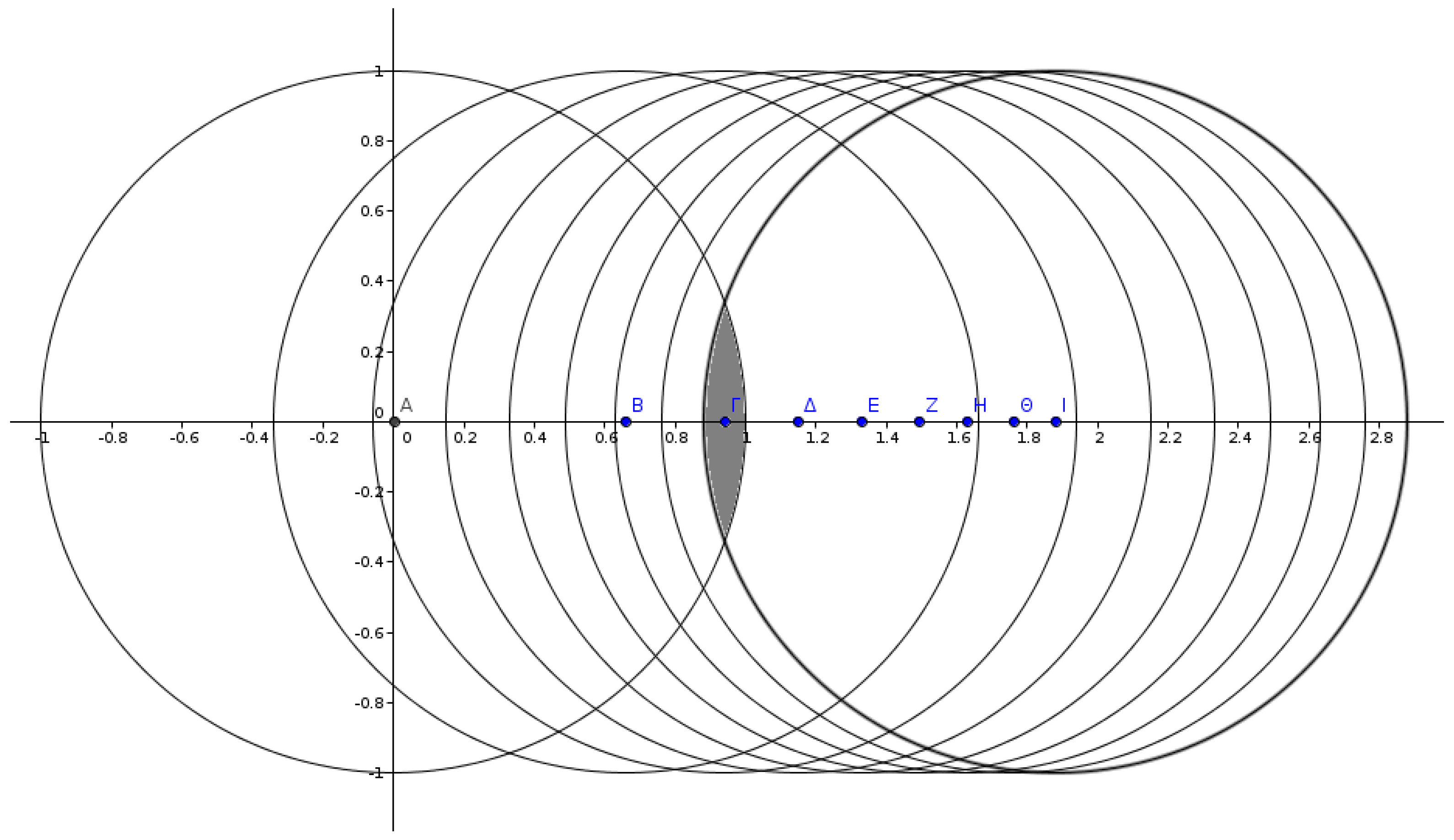
Figure 2.
This figure depicts the evolution of C(t) (i.e., network coverage) over time for a geometric random graph of 1000 nodes using the random walker mechanism. The curves produced using Equation (5) (for various values of ) are close to the one produced using Equation (7), except from the red curve that corresponds to the smallest , which is where the network is marginally connected.

Figure 3.
A snapshot of a geometric random graph with and transmission range . It depicts a marginally-connected WSN from which it can be visually understood why there is a significant time lag in the network coverage of a random walker, compared to denser networks. One can easily observe the existence of small bottlenecks dispersed over the network.

Figure 4.
Mean number of neighbors depending on the radius for a geometric random graph of 1000 nodes.
Figure 4.
Mean number of neighbors depending on the radius for a geometric random graph of 1000 nodes.

Figure 5.
A bar graph showing the spatial displacement of the random walker after each step on a network with nodes and = 0.05. There are steps, and each bar corresponds to the number of steps (×50), where the spatial displacement of the random walker is in the range of .
Figure 5.
A bar graph showing the spatial displacement of the random walker after each step on a network with nodes and = 0.05. There are steps, and each bar corresponds to the number of steps (×50), where the spatial displacement of the random walker is in the range of .

Figure 6.
Random walker’s spatial displacement from the starting node. The blue line is from the analytical part of this study (i.e., Equation (1)), while the red one is from the simulation results. One can see that the walker is permitted to move in all directions; hence, the distance from the starting node could be either decreased or increased.

Figure 7.
Simulation results for 100 sparse networks with number of nodes , radius and mean number of neighbors . One can see that the simulation’s outcome is in accordance with the expected results from the analysis.
Figure 7.
Simulation results for 100 sparse networks with number of nodes , radius and mean number of neighbors . One can see that the simulation’s outcome is in accordance with the expected results from the analysis.
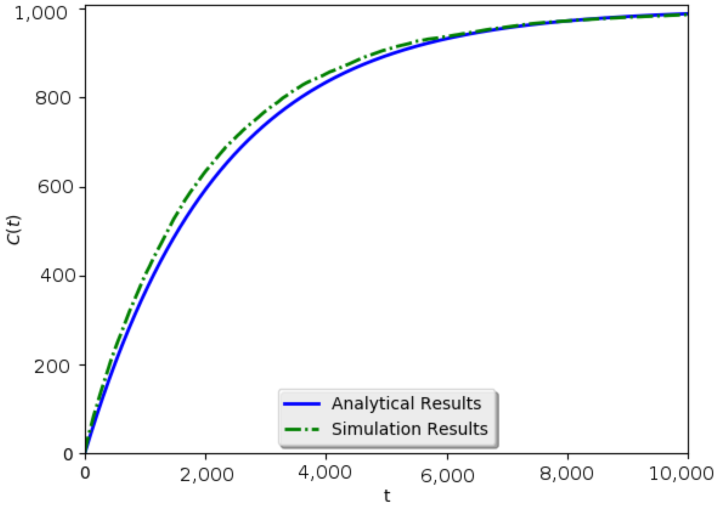
Figure 8.
Simulation results for networks of various densities of links , (red), 0.200 (green), 0.500 (magenta), 1.000 (yellow), number of neighbors . It depicts the coverage over the number of time steps. Full lines are for the analytic results and dashed for simulation results. Similarly to previous outcomes, the modeling is in accordance with the simulation. Moreover, it is clear that there is a difference only in the case of marginally-connected networks with the minimum value for radius .

Figure 9.
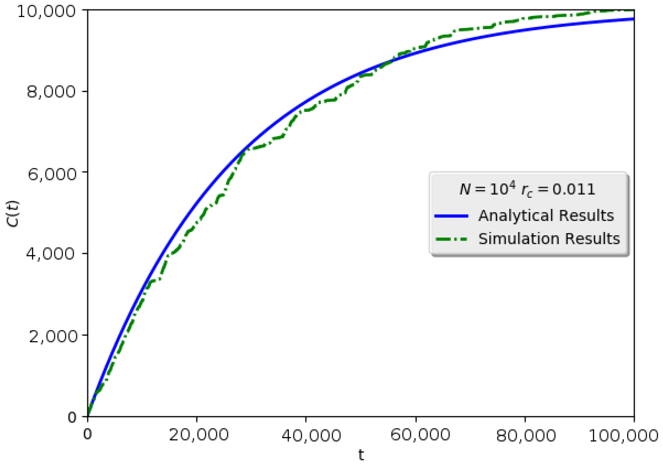
Simulation results for the grid geometric network (green dashed line), , , mean number of neighbors . Coverage is depicted over the number of time steps. There is a strong correlation between the analytical part and the simulation one.
Figure 9.
Simulation results for the grid geometric network (green dashed line), , , mean number of neighbors . Coverage is depicted over the number of time steps. There is a strong correlation between the analytical part and the simulation one.

Figure 10.
Simulation results for the grid geometric network, , , mean number of neighbors . Similarly to the previous simulation results, there is a fit between the modeling and simulation.
Figure 10.
Simulation results for the grid geometric network, , , mean number of neighbors . Similarly to the previous simulation results, there is a fit between the modeling and simulation.

© 2017 by the authors. Licensee MDPI, Basel, Switzerland. This article is an open access article distributed under the terms and conditions of the Creative Commons Attribution (CC BY) license (http://creativecommons.org/licenses/by/4.0/).
Share and Cite
MDPI and ACS Style
Skiadopoulos, K.; Giannakis, K.; Oikonomou, K. Random Walker Coverage Analysis for Information Dissemination in Wireless Sensor Networks. Technologies 2017, 5, 33. https://doi.org/10.3390/technologies5020033
AMA Style
Skiadopoulos K, Giannakis K, Oikonomou K. Random Walker Coverage Analysis for Information Dissemination in Wireless Sensor Networks. Technologies. 2017; 5(2):33. https://doi.org/10.3390/technologies5020033
Chicago/Turabian StyleSkiadopoulos, Konstantinos, Konstantinos Giannakis, and Konstantinos Oikonomou. 2017. "Random Walker Coverage Analysis for Information Dissemination in Wireless Sensor Networks" Technologies 5, no. 2: 33. https://doi.org/10.3390/technologies5020033
Note that from the first issue of 2016, this journal uses article numbers instead of page numbers. See further details here.