
Fréchet Distribution Applied to Salary Incomes in Spain from 1999 to 2014. An Engineering Approach to Changes in Salaries’ Distribution


1
Instituto Universitario de Microgravedad “Ignacio Da Riva” (IDR/UPM), ETSI Aeronáutica y del Espacio, Universidad Politécnica de Madrid, Pza. del Cardenal Cisneros 3, 28040 Madrid, Spain
2
Colegio de Ingenieros de Caminos, Canales y Puertos, Colegiado n° 13177, Almagro 42 - 1a Planta, 28010 Madrid, Spain
*
Author to whom correspondence should be addressed.
Economies 2017, 5(2), 14; https://doi.org/10.3390/economies5020014
Submission received: 20 December 2016
/
Revised: 9 April 2017
/
Accepted: 18 April 2017
/
Published: 1 May 2017
Abstract
:The official data in relation to salaries paid in Spain from 1999 to 2014 has been analyzed. The inadequate data format does not reflect the whole salary distribution. Fréchet distributions have been fitted to the data. This simple distribution has similar accuracy in relation to the data when compared to other distributions (Log-Normal, Gamma, Dagum, GB2). Analysis of the data through the fitted Fréchet distributions reveals a tendency towards more balanced (i.e., less skewed) salary distributions from 2002 to 2014 in Spain.
Keywords:
Spanish economy; salary distribution; parametric modelling; Fréchet distribution; minimum wageJEL Classification:
C22; J311. Introduction
In November 2015, the salary distribution data in Spain was updated in the statistics database of the Spanish Tax Agency.1 This data is organized by taking into account several aspects of the Spanish society (gender, age, economic sectors, etc.). According to the best-selling newspaper in Spain,2 the most significant information was the salaries earned in relation to the salary brackets (see in Table 1 and Table 2 the number of salaried people and its weight in terms of total amount of paid euros, in relation to the salary, expressed in times the minimum wage), which demonstrates that the average annual salary in Spain fell in 2014 to the levels of 2007. Other key information from the statistics reflected in the media was the imbalance between genders.3
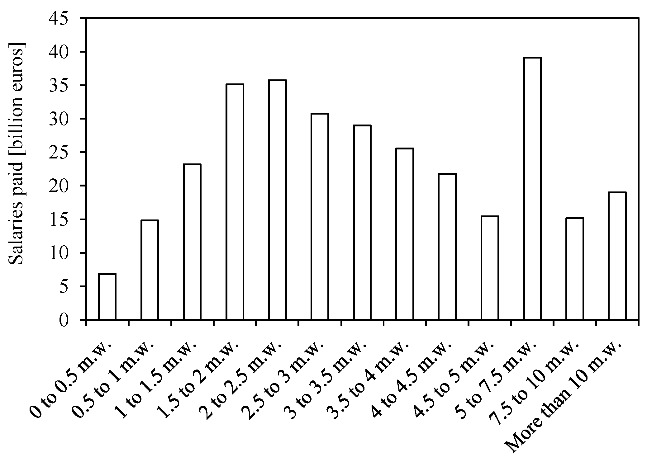
The aforementioned statistical information (included in Table 1 and Table 2) is organized in brackets of half minimum wage size until five times the minimum wage. This wage limit is followed by a bracket from 5 to 7.5 times the minimum wage and then by a bracket from 7.5 to 10 times the minimum wage. Finally, the statistics end with a more than 10 times the minimum wage bracket. In Figure 1, the distribution of the salaries paid is shown as a function of the salary bracket in 2014. A significant concern arises from this figure, as the different size of the brackets does not allow for fitting a mathematical distribution in order to obtain more information from the data.
The aim of the present work is to draw some conclusions from this data based on the empirical analysis normally used by engineers and scientists when studying a problem, which requires the use of mathematical models that can be parametrized in terms of a limited number of non-dimensional variables. This approach facilitates working with distributional functions that retain the most significant information reflected by the data. In addition, the possibility of defining the aforementioned functions from a limited amount of data (e.g., surveys) should be also mentioned as one of the main advantages of this methodology. To perform the present study:
- (1)
- The data from Table 1 and Table 2 was post-processed in order to obtain an estimation of the salaries earned in brackets of half minimum wage from 5 to 7.5 times the minimum wage and from 7.5 to 10 times the minimum wage. To do this, the evolution of the minimum wage in Spain from 1999 to 2014 is required (see Table 3).
- (2)
- The data (salaries paid) was made non-dimensional in order to directly compare the distributions from different years.
- (3)
- A corrected Fréchet distribution was fitted to the data (once post-processed), the evolution from 1999 to 2014 of this distribution being analyzed in order to detect changes in their main parameters and study the data through them.
The three-parameter Weibull distribution (Weibull 1951) was initially proposed to model the salary distribution in the present work. This is a simple but versatile distribution widely used in wind engineering and wind energy assessment (Justus et al. 1978; Rehman et al. 1994; Lun and Lam 2000; Seguro and Lambert 2000; Dorvlo 2002; Ulgen and Hepbasli 2002; Azad et al. 2014; Shittu and Adepoju 2014). The corrected Weibull probability density function (PDF) is expressed as:
where c is the scale parameter, k is the shape parameter, and d is the location parameter (Cran 1988). The correction parameter, λ, is used in order to obtain a better fit to the data, bearing in mind that the salaries interval is half minimum wage, and, therefore, the value of this parameter should be approximately λ = 0.5. In the present study, the function f stands for the density of salaries earned, whereas the variable φ stands for the salary (expressed in terms of times the minimum salary). However, the results of the fittings performed in the present work showed negative values of the shape and correction parameters. For this reason, the Fréchet distribution, which is closely related to the Weibull distribution (Abbas and Tang 2012; Mann 1984; De Gusmão and Ortega 2011; Khan et al. 2008), was finally selected.4 The Fréchet distribution is expressed as:
where, as aforementioned, c is the scale parameter, γ is the shape parameter, and d is the location parameter. Obviously, once the scale parameter is proven to be c > 0, it is easy to derive Equation (2) from Equation (1) by assuming γ = −k. Both aforementioned distributions, Weibull and Fréchet, are commonly applied to analyze the extreme values from other probability distributions (Goda et al. 2010; Carmona 2014) and represent the Fisher-Tippett FT-III and FT-II distributions, respectively (Fisher and Tippett 1928).
After a review of the available literature, it seems that the Weibull or Fréchet distributions are not commonly used in economics, compared to other distributions. Nevertheless, some examples of the use of these distributions have been found; for example, to describe the income distribution in a society (Chotikapanich et al. 2007; Jagielski and Kutner 2013; Atkinson and Bourguignon 2015) or the inequality associated with that distribution (Krause 2014; McDonald and Ransom 2008; Lubrano 2016). In the present work, the analysis is focused on wages, leaving aside other revenue types normally included in the analysis of incomes or wealth.
Just focusing on wages, the recent work by García et al. (2014) is worthy of mention. These authors analyze different PDFs to study some specific aspects of the salary distributions is Spain, suggesting the use of the four-parameter GB2 distribution as the best choice when fitting to the data. However, in that work, the reference data is obtained from the National Statistics Institute of Spain (Instituto Nacional de Estadística) annual survey, whereas in the present analysis the raw data is based on the entire database from the Spanish Tax Agency. In addition, the PDFs analyzed seem to be quite complicated when compared to the Fréchet distribution equation. Therefore, in the present work the authors have followed the suggestion by Banerjee et al. (2006), who stated ‘that a useful description of the data is the one that has the minimal number of parameters, yet reasonably (but not necessarily perfectly) agrees with the data’.
Together with the aforementioned work by García et al. (2014), a few examples in the available literature related to distributions applied to analysis of wages have been found. Shatnawi et al. (2013) studied gender discrimination in relation to wages.5 These authors stated that the wage density distribution related to a specific group of individuals (in this case male workers) corresponds to the log-normal distribution. In this sense, Benoit Mandelbrot in his work ‘Paretian distributions and income maximization’,6 stated some decades before that different distributions of offers (i.e., wages) made to a single individual are conditioned by how each sector weights the attributes of this individual (Mandelbrot 1962). Therefore, in a whole economic system there is a coexistence of distributions that affect different social groups. An example of this mixture of density functions has been recently proposed to model wage distributions in the Czech Republic (Marek and Vrabec 2013). In addition, works by Rigby and Stasinopoulos (2015), Machado and Mata (2005), and Sohn et al. (2014) can also be mentioned.7 In these works, a procedure to fit a mixture of distributional functions is developed, the works by Machado and Mata (2005), and Sohn et al. (2014) being respectively applied to wage distribution in Portugal from 1986 to 1995 and in Germany (years 1992 and 2010). These procedures have helped to analyze how inequality affects different subgroups of the population studied.
The Spanish economy has undergone drastic changes in the last 15 years. The evolution of the salaried people from 1999 to 2014 is included in Figure 2, together with the evolution of the total amount of salaries earned. After the crisis from 1994 to 1999, the Spanish economy boomed and unemployment fell. From 2006, the Spanish economy suffered the longest crisis within the period of democracy (i.e., from 1977) (Galindo 2015). This has affected the salary distribution in relation to the salary earned, thereby widening this distribution as a result of the demand for highly skilled workers, which increases the effect of the college premium for the high salaries (Carrasco et al. 2015). This conclusion had already arisen with regard to the 1994–1999 crisis (Febrer and López 2004). In contrast, inequality had fallen in the previous period, from 1985 to 1992, as a result of the unemployment reduction and the decrease in the college premium earnings for the high-skilled jobs (Pijoan-Mas and Sánchez-Marcos 2010). Inequality as a consequence of the present crisis has been the focus of many researchers’ attention, the most noteworthy example in terms of interest generated in all establishments around the world (political, economic, academic…) being the work by Thomas Piketty ‘El Capital en el Siglo XXI’ (Capital in the Twenty-First Century) (Piketty 2014).8 Regarding the Spanish economy, it seems that the adjustment is far from being fair in terms of society wealth (Orsini 2014).
As mentioned, the purpose of the authors is to analyze the salary distributions in Spain from their point of view as engineers and researchers (Cubas et al. 2014a; Mendaña and Pindado 2013; Pindado et al. 2015; Pindado et al. 2013; Cubas et al. 2014b), relying only on mathematical modeling of the data and using the Fréchet distribution. In addition, the authors have tried to work as far as possible from the constant echoes coming from different ideologies that try to explain the origin of the present economic crisis in Spain and its possible solution. Wages and distribution of wealth or incomes are not completely dependent on one another, other factors such as education or household economic structure also being important for wealth sharing in a modern society (Espejo and Pascual 2007; Asplund and Barth 2005). In terms of the intellectual challenge involved in post-processing and understanding the data, the authors find the present moment of the economy fascinating. However, let us also say that, focusing only on cold mathematical modeling, we are well aware of the difficulties many Spanish people have in finding anything fascinating about the present situation of the economy.
2. Methodology
To estimate the total earned salary corresponding to sub-brackets of half minimum wage from 5 to 7.5 times the minimum wage and from 7.5 to 10 times the minimum wage, two assumptions are made:
- the number of salaried people depends linearly on the salary, and
- the average salary corresponding to each new sub-bracket of half minimum wage is centered in relation to the aforementioned bracket.
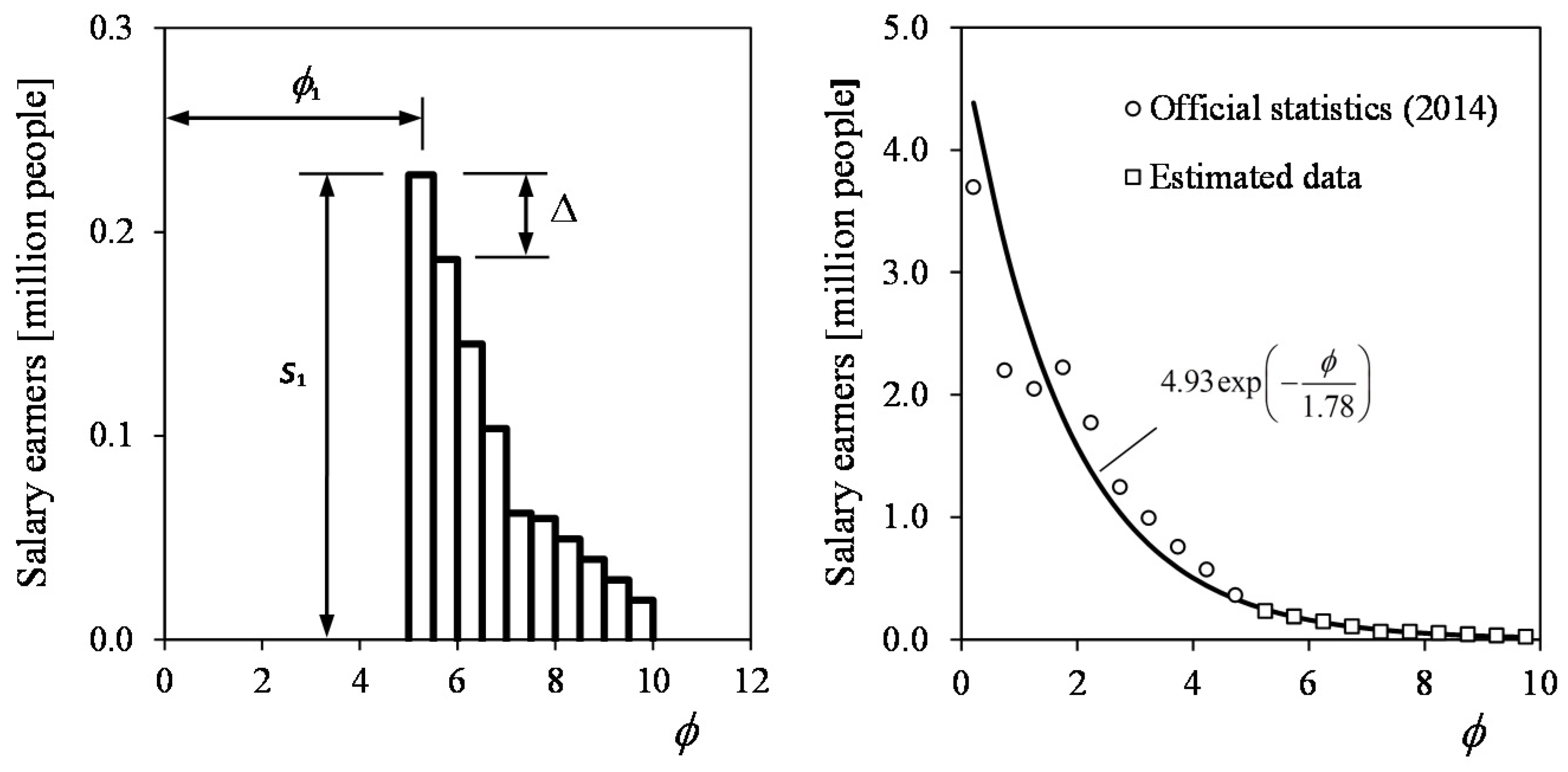
The linear distribution in each bracket is characterized by the number of salaried people in the first sub-bracket, s1, and the reduction in the number of earners from one sub-bracket to the following one, Δ. Therefore, if S is the population (salaried people) within the bracket to be split into five new sub-brackets, M is the total amount of salaries paid in the brackets to be split, Φ is the annual minimum wage, and φ1 is the center of the first sub-bracket (φ1 = 5.25 times the minimum wage in the case of the 5 to 7.5 times the minimum wage salaries bracket and φ1 = 7.75 times the minimum wage in the case of the 7.5 to 10 times the minimum wage salaries bracket, see Figure 3), the following expressions can be derived for Δ and s1:
Therefore, the salaried people within each sub-bracket j can be expressed as:
The salary earners in each half-minimum wage sub-brackets from 0 to 10 times the minimum wage are also shown for 2014 in Figure 3. Once the number of earners in each sub-bracket has been estimated, the amount of salaries paid can be calculated by multiplying this quantity by the salary corresponding to the center of the sub-bracket. In Figure 4, the salary distribution corresponding to 2014 (made non-dimensional by dividing by the total amount of salaries paid that year), is shown. In this graph the open circles correspond to the data from Table 1 and Table 2, whereas open squares correspond to the calculated data with Equations (3) to (5). It should also be mentioned that other more complex approaches to the data within the studied brackets (quadratic or cubic distributions, instead of the linear ones) are possible.
Furthermore, it can be observed in the right graph of Figure 3 that an exponential equation:
fits the distribution of salary earners, s, as a function of the salary earned expressed in number of times the minimum salary, φ, well. From this expression, it is possible to estimate the salary earners in the bracket between φ1 and φ2 minimum salaries:
It should be mentioned that the factor of 2 included in the expression above is necessary, as the data is discretized in terms of half minimum wage. Equation (7) gives the total amount of salaried people in 2014 with a 3.9% error rate.
The Fréchet Distribution Fitted to the Data
The proposed Fréchet distribution (i.e., Equation (2)), reproduced here for convenience:
has been fitted to the normalized distribution of 2014 salaries earned in relation to the non-dimensional minimum wage, φ, see Figure 4. Fitting was performed with the least squares method using MATLAB. As can be observed in the figure, the correlation seems to be accurate. Other PDFs used in income analysis (Atkinson and Bourguignon 2015; Kleiber and Kotz 2003; McDonald and Ransom 1979; Klein et al. 2015) such as the log-normal distribution:
the gamma distribution:
and the Dagum distribution (Kleiber 2008):
have been also fitted to the data with good results. Furthermore, the GB2 distribution mentioned in the first section (García et al. 2014):
was also included in the study in order to compare the suggested approach with a more complex (and better)9 distribution. The above PDFs have been compared, for the 2014 data, with the proposed Fréchet distribution in terms of Root Mean Square Error (RMSE):
where yn is the percentage of the salaries paid at the income bracket corresponding to the salary φn and f (φn) is the figure from the selected PDF at φn. The results show similar values of this error (RMSE = 4.423 × 10⁻² [Fréchet]; RMSE = 4.410 × 10⁻² [log-normal]; RMSE = 4.443 × 10⁻² [gamma]; RMSE = 4.415 × 10⁻² [Dagum]; and RMSE = 4.403 × 10⁻² [GB2]) for the five distributions.
Once Equation (8) is fitted to the data, it is possible to estimate the salaries paid in the bracket between φ1 and φ2 minimum salaries:
where TSP is the total amount of salaries paid (TSP = 311.28 billion euro in 2014, see Table 2). As aforementioned, the factor of 2 included in the expression above is necessary because the data is discretized in terms of half minimum wage. Equation (14) gives the total amount of salaries paid in 2014 with a 4.6% error rate (calculated from φ = 0 to φ → ∞, that is, leaving aside the contribution within the bracket [d, 0] [the location parameter, d, has a negative value in all studied cases]).
3. Results and Discussion
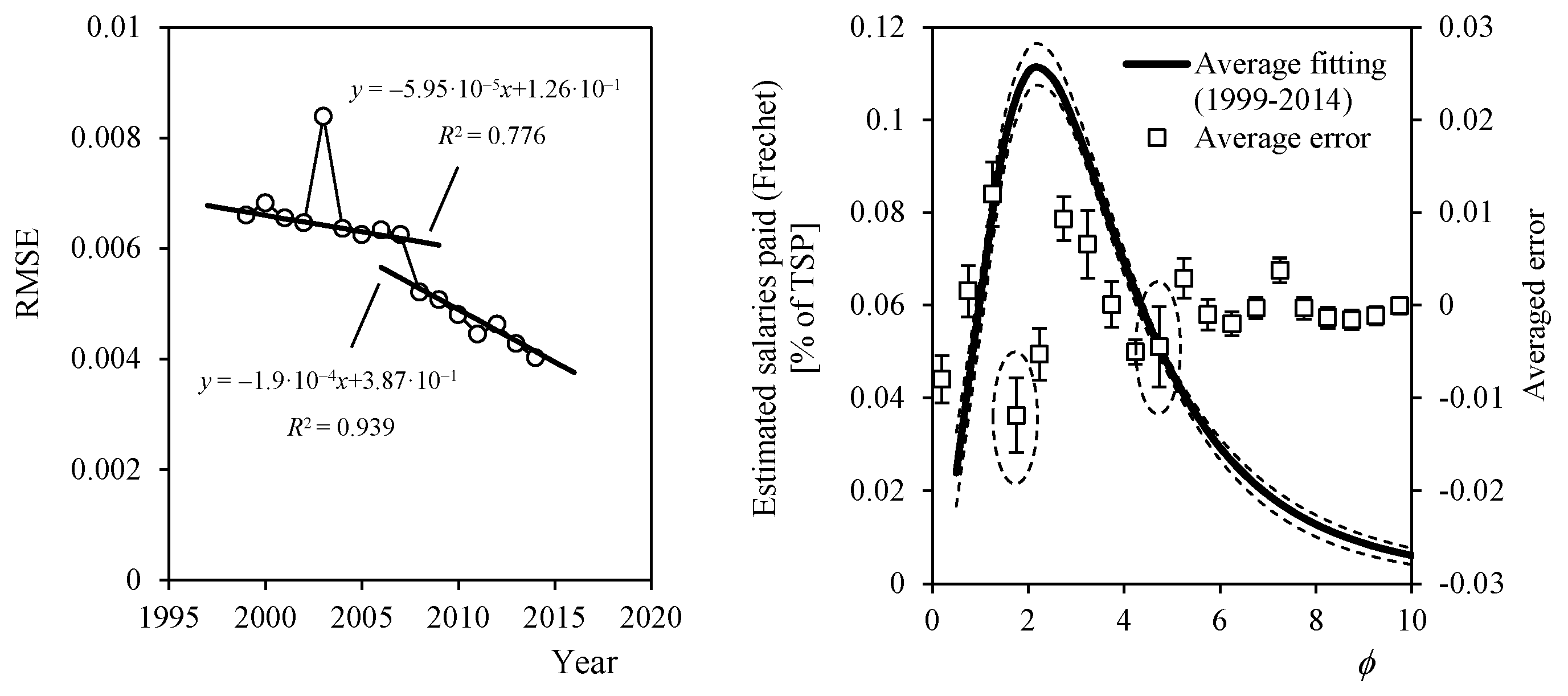
In Table 4, the coefficients resulting from the salary earners and the salaries paid distributions (Equations (6) and (8), respectively) from 1999 to 2014 are included. These results are shown in the graphs of Figure 5. As expected, the lower graph of the figure reveals the same progressive change regarding the salaries paid from 2008 as the one reflected in Figure 2. The coefficients have a local variation in 2003. The RMSE evolution of the proposed Fréchet distribution calculated in relation to the data (Equation (13)) is plotted in Figure 6 (left). The results indicate that this distribution comes closer to the statistical data, as it shows decreasing values of the RMSE from 1999 to 2014. A higher value of this error is locally reached in 2003, reproducing the local variation shown in Figure 5. This might be explained by the removal of the restriction in relation to the hiring of civil servants by both the central and regional authorities in Spain (Argimón and Gómez 2006) (it should be mentioned that the importance of the public servants in the statistics is significant). As an example, the number of civil servants in Spain represented 14.1% of total salary earners and 19.4% of the salaries paid in 2004 (Botella et al. 2009). Moreover, the total weight of the public sector on the Gross Domestic Product in Spain has been estimated to be approximately 45%).10 In addition, two distinct patterns are shown by the evolution of the RMSE in the aforementioned graph. From 1999 to 2007, a slightly decreasing pattern is shown, whereas from 2008 the negative slope of that pattern is accentuated. This effect could be the result of the changes in the labor market law implemented in 2010 and 2012 in Spain (without leaving aside the changes faced by the Spanish economy since the beginning of the present crisis in 2007).11
In addition, the curve formed by the averaged values (from 1999 to 2014) of the percentage salaries paid, estimated through the fitted Fréchet distributions, is shown in Figure 6 (right), together with the curves that represent the maximum and minimum values, plotted with dashed lines. Also, the averaged differences (averaged error) between the Fréchet distribution and the official statistical data at all 0.5 minimum wage brackets are plotted in this graph from 1999 to 2014. It can be said that, although based on the results (Figure 4), the Fréchet distribution fits the data well, some degree of error is locally shown. However, the fact that the proposed wages distribution, once fitted to the data, represents several different groups of individuals (with different skills and different evaluation of them), should be taken into account when trying to explain these differences. Finally, one more effect can be observed in this graph. A higher deviation, related to the differences between the fitted distribution and the official data, is shown for φ = 2 and φ = 5, suggesting a boundary between groups of salaried people and indicating two possible changes from one year to the next; in money (i.e., the salary payed to the people at one side of this boundary has changed) or in people (i.e., some people have moved, increasing or decreasing their salary, to the other side of the boundary).12
In order to analyze the data from Table 1 and Table 2 and estimate the accuracy of the proposed analytical approach, the number of salaried people responsible for the amount of salaries paid are placed in three different brackets: 0%–30%, 30%–70%, and more than 70%. From Equation (14), the following expressions can be derived for the salaries that represent the boundaries between the three brackets, φ30% and φ70%:
Once the aforementioned boundary salaries, φ30% and φ70%, are calculated, the salaried people in the brackets mentioned in Equation (7) can be estimated:
The results (in terms of percentage in relation to the total amount of salary earners each year) are included in Table 5 and Figure 7. It can be observed that the results based on the analytical approximation follow the general trend shown by the results calculated with direct interpolations on the statistical data from Table 1 and Table 2. However, a noteworthy deviation of the analytical approximation can also be observed in the graph.
Another interesting result is observed when the annual increases on the salaried people within the 0%–30% and 30%–70% brackets (respectively, Δ0%–30% and Δ30%–70%) are compared. The data shows a very good correlation indicating that each increase (decrease) in the number of earners within the 0%–30% salaries paid bracket is well correlated with a proportional decrease (increase) in the number of earners within the 30%–70% salaries paid bracket (see right graph of Figure 7). As it can be observed in Table 5, the boundary salary φ30% has a value of approximately φ30% = 2, which was identified as one of the points where a higher transfer of salaried people from one side to the other of this salary level was produced from 1999 to 2014. The estimated results (based on the Fréchet distribution fitting), however, do not reflect the aforementioned correlation. In addition, it should also be said that, according to the graph in Figure 7, the percentage of earners within the more than 70% salaries paid bracket remains constant throughout the studied period (1999–2014).
Finally, the distribution of the salaries paid can be studied in terms of skewness; that is, the asymmetry of the distribution (or the difference between both tails weight). The skewness, skw, of the Fréchet distribution is calculated using the gamma function (De Gusmão and Ortega 2011; Khan et al. 2008):
However, to analyze the asymmetry of the fittings and its evolution within the studied period, a simpler parameter was selected. This asymmetry parameter, ψ, is defined as the difference between the median:
and the mode:
of the distribution. Therefore:
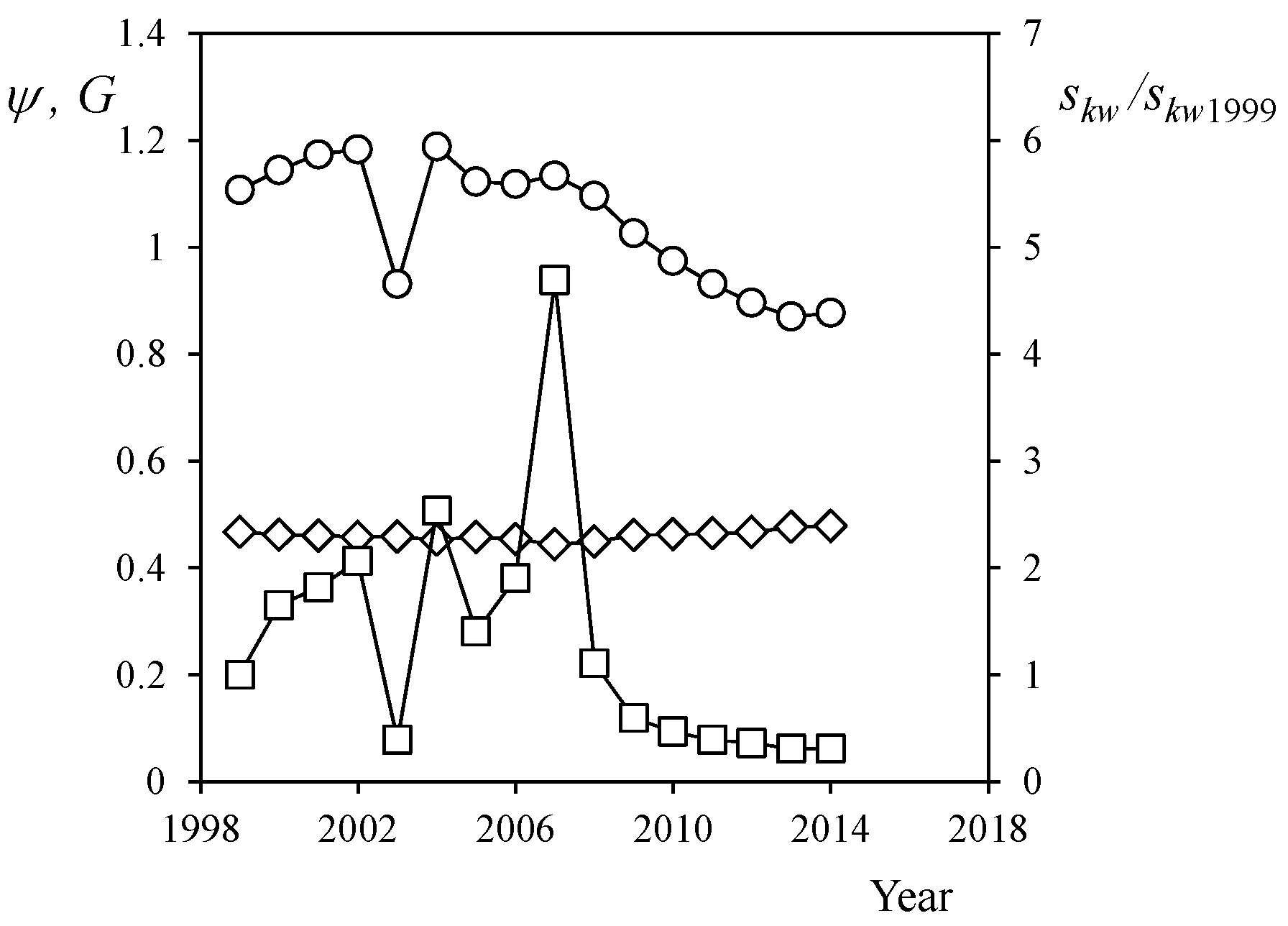
With this definition of the asymmetry, we have defined a parameter that would help to measure how much the salaries paid distribution detach from a normal (or Gaussian) distribution, which is characterized by zero skewness (and equal values of the mode and the median). A normal distribution of the salaries would be more heavily weighted on the middle wage levels, with equally weighted tails (i.e., the weight of the large number of low wages counterbalances the weight of the low number of high wages). In Figure 8, the results are shown. Leaving aside the result from 2003, produced by a larger error of the fitting from the official statistics data that year, it can be said that after a quite constant level of asymmetry from 1999 to 2007, ψ = 1.11–1.18, the asymmetry falls to 0.87 in 2013–2014. Hence, the results seem to indicate that a more balanced salary distribution was reached in 2013–2014, after the booming years of the Spanish economy (from 1999–2007). Finally, it should be underlined that this transition towards a less unequal salary distribution sharply contrasts with the latest reports on inequality in Spain regarding incomes and wealth.
In order to check the robustness of the present analysis, some additional calculations were carried out. Firstly, the skewness, skw, was calculated in order to compare it with the suggested symmetry parameter, ψ. The results, made non dimensional with the value of the skewness in 1999, are also included in Figure 8. A similar trend between the skewness and parameter ψ can be observed. In addition, it seems that parameter ψ can filter some noise shown by the skewness in those points where the scale parameter, γ, is close to γ = 3, as the skewness of the Fréchet distribution presents a singularity at this point.
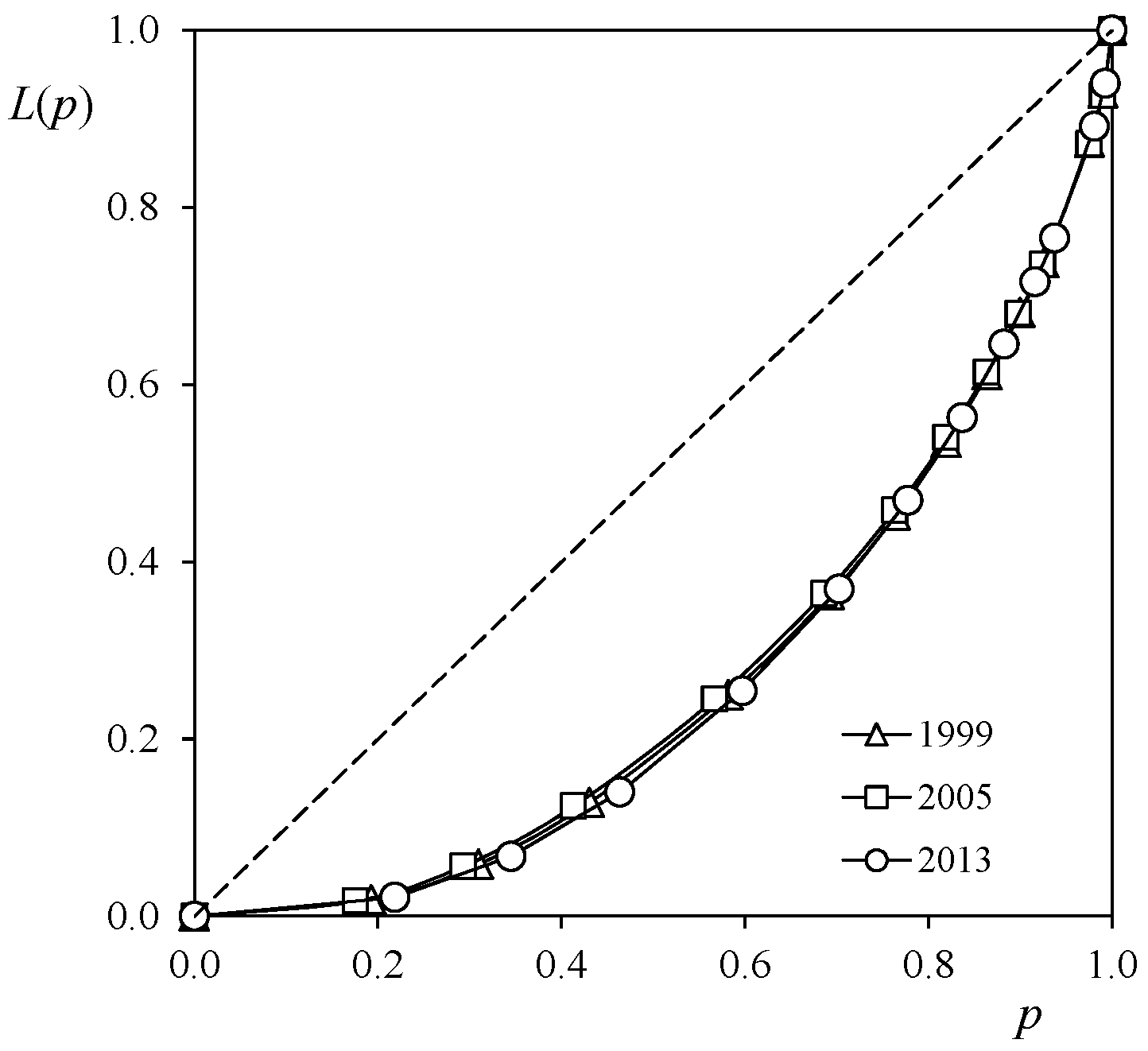
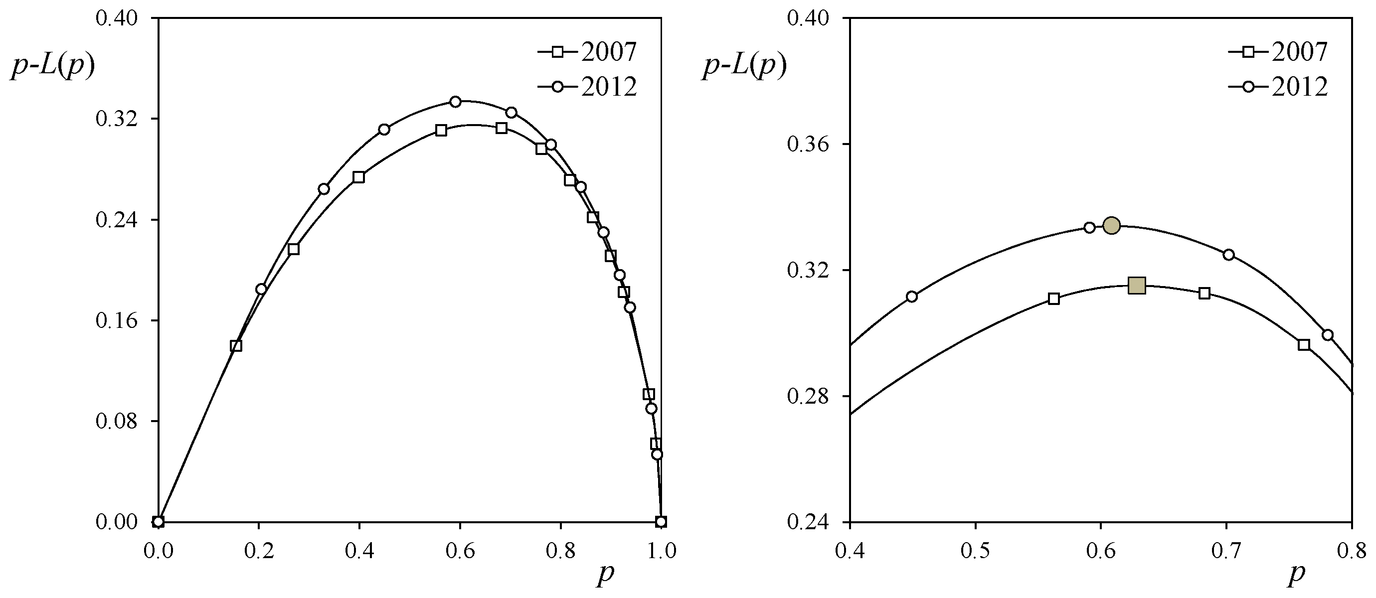
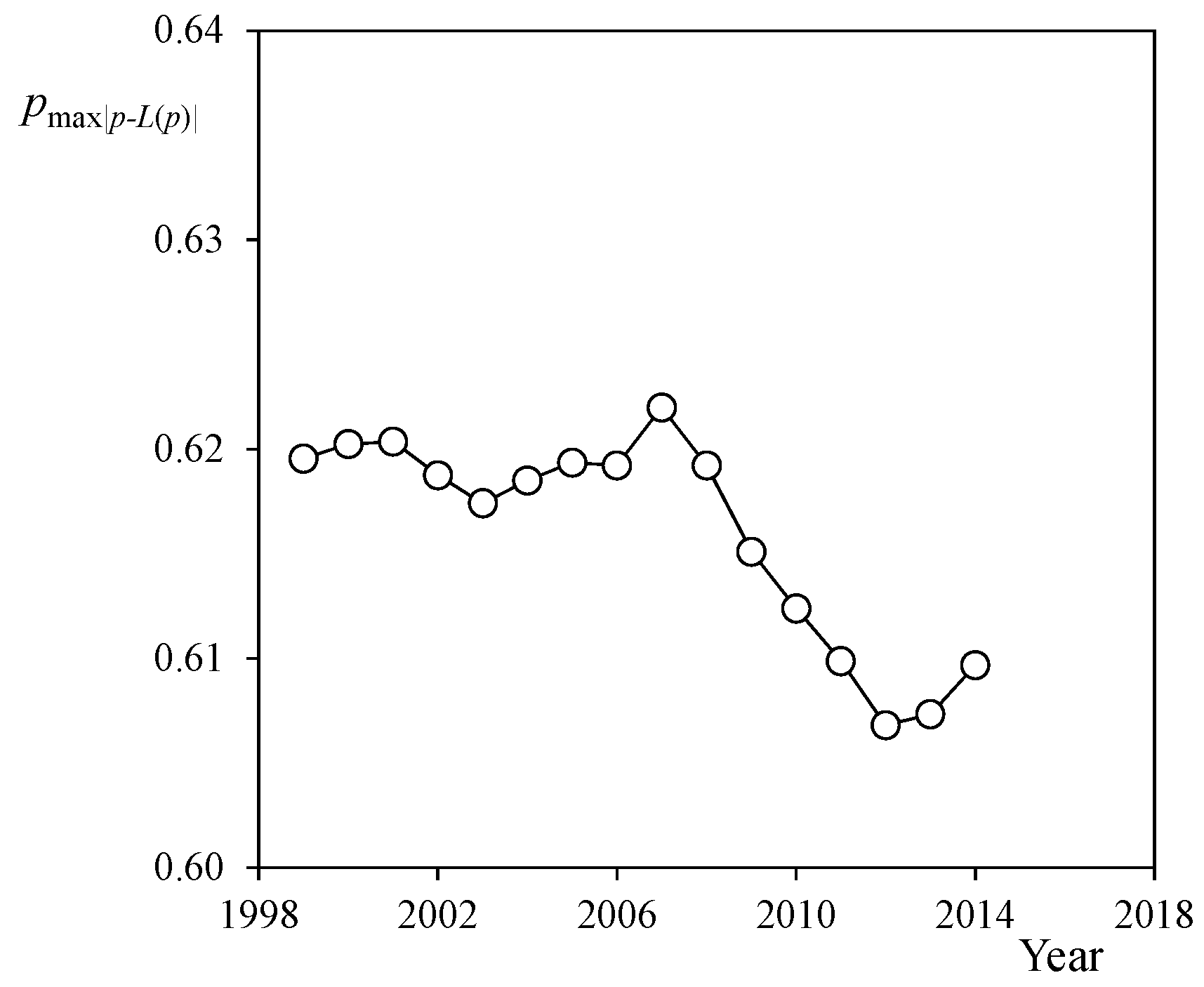
Secondly, the evolution of the wages distribution was analyzed using the Lorenz curves. This approach is normally applied to income inequality (Krause 2014; Lubrano 2016). According to Lubrano (2016), the Lorenz curve is ‘a graphical representation of the cumulative income distribution. It shows for the bottom p1% of households, what percentage p2% of the total income they have’. In Figure 9, the Lorenz curves corresponding to 1999, 2005, and 2013 are shown. In this graph, the percentage of the salaried people, p, is plotted on the x-axis, whereas the percentage of the wages received by this number of salaried people, L(p), is plotted on the y-axis. The Lorenz curves were calculated, from 1999 to 2014, with the data from Table 1 and Table 2. As can be observed in Figure 9, all curves have the same pattern. Nevertheless, some additional information can be derived in order to establish an evolution pattern followed by the wages distribution. If the difference between the Lorenz curve and the theoretical values that represent the maximum equality (Krause 2014), p − L(p), is plotted as a function of the percentage of the salaried people, p, it is possible to analyze the position of the maximum of this curve (see Figure 10). If this maximum is displaced towards p = 1, the existence of an elite within the salaried group is revealed, whereas if it is displaced towards p = 0 it could be said that a group with extreme low wages exists. The evolution of this maximum position, pmax|p− L(p)|, from 1999 to 2014 is shown in Figure 11. It can be appreciated that this maximum detaches its position from p = 1, which indicates a reduction in the importance of the higher wages (the elite) in relation to the whole group. This result agrees with the pattern shown by the symmetry parameter ψ in Figure 8; that is, the salary distribution in Spain has changed towards a more balanced situation since 2007.
Finally, we have performed a further analysis of the data, studying the evolution of the Gini coefficient, G, defined as (Krause 2014; Lubrano 2016):
The evolution of this coefficient, G, between 1999 and 2014 has been plotted in Figure 8 in order to compare it with the evolution of the defined asymmetry parameter, ψ, and the skewness, skw. It seems that the value of this coefficient remains quite constant, with a very slight increase starting in 2007, indicating an increase of inequality. This result contrasts with the previous results, based on the asymmetry of the wage distributions, and indicates a margin for further research.
4. Conclusions
In the present work, the official data in relation to salaries paid in Spain from 1999 to 2014 has been analyzed. The Fréchet distribution was used as a way of studying the data using an analytic expression that depends on a limited number of parameters. The most significant conclusions resulting from this work are:
- The Fréchet distribution has proven to fit the studied salaries’ distributions well, having a similar accuracy in relation to the data when compared to other distributions (Log-Normal, Gamma, Dagum, GB2) that can be considered more complex.
- The analysis of the results showed that changes in the salary distribution as a result of the economy evolution are reflected in the 0%–30% and 30%–70% brackets of the total salaries paid, the top 30% (affecting 9% of the salaried people) being quite resilient to those changes from 2002 to 2014 in Spain.
- Finally, the results based on the distributions’ asymmetry (skewness) indicate an increasingly more balanced salaries distribution (i.e., less skewed) starting in 2007. However, this seems to be in contrast with the evolution of the Gini coefficient.
Acknowledgments
The authors are truly grateful to Brian Elder and Anthony Maldonado for their kind help with improving the style of the text. The authors would also like to thank the referees for their help in improving the present work.
Author Contributions
Santiago Pindado and Carlos Pindado had the idea for this research. Carlos Pindado collected all the data whereas Santiago Pindado was responsible for the analytical modeling. Javier Cubas programmed the curve fittings. All authors were equally involved the literature review.
Conflicts of Interest
The authors declare no conflict of interest.
References
- Abbas, Kamran, and Yincai Tang. 2012. Comparison of Estimation Methods for Frechet Distribution with Known Shape. Caspian Journal of Applied Sciences Research 1: 58–64. [Google Scholar]
- Alonso, Mario. 2016. El sector público en España está poco auditado. El País, January 3. Available online: http://economia.elpais.com/economia/2015/12/29/actualidad/1451383564_744232.html (accessed on 21 April 2017).
- Argimón, Isabel, and Ángel Luis Gómez. 2006. Empleo y salarios en las AAPP : Una perspectiva macroeconómica. Revistas. Presupuesto Y Gasto Público 41: 73–92. [Google Scholar]
- Asplund, Rita, and Erling Barth, eds. 2005. Education and Wage Inequality in Europe. A literature Review. Helsinki: ETLA. [Google Scholar]
- Atkinson, Anthony B., and François Bourguignon. 2015. Handbook of Income Distribution. Amsterdam: Elsevier B.V. [Google Scholar]
- Azad, Abul Kalam, Mohammad Golam Rasul, and Talal Yusaf. 2014. Statistical Diagnosis of the Best Weibull Methods for Wind Power Assessment for Agricultural Applications. Energies 7: 3056–85. [Google Scholar] [CrossRef]
- Banerjee, Anand, Victor M. Yakovenko, and T. Di Matteo. 2006. A study of the personal income distribution in Australia. Physica A: Statistical Mechanics and its Applications 370: 54–59. [Google Scholar] [CrossRef]
- Botella, Marta, Pablo Hernández de Cos, and Javier J. Pérez. 2009. Algunas consideraciones sobre los efectos macroeconómicos de los salarios y del empleo de las Administraciones Públicas. Boletín Económico. Banco de España 9: 57–74. [Google Scholar]
- Burkhauser, Richard V., and Kenneth A. Couch. 2009. Intragenerational inequality and intertemporal mobility. In The Oxford Handbook of Economic Inequality. Edited by Wiemer Salverda, Brian Nolan and Timothy M. Smeeding. New York: Oxford University Press, pp. 522–45. [Google Scholar]
- Carmona, René. 2014. Statistical Analysis of Financial Data in R. New York: Springer. [Google Scholar]
- Carrasco, Raquel, Juan F. Jimeno, and A. Ortega. 2015. Returns to Skills and the Distribution of Wages: Spain 1995–2010. Oxford Bulletin of Economics and Statistics 77: 542–65. [Google Scholar] [CrossRef]
- Chotikapanich, Duangkamon, D. S. Rao, and Kam Ki Tang. 2007. Estimating income inequality in China using grouped data and the generalized beta distribution. Review of Income and Wealth 53: 127–47. [Google Scholar] [CrossRef]
- Cran, G.W. 1988. Moment estimators for the 3-parameter Weibull distribution. IEEE Transactions on Reliability 37: 360–63. [Google Scholar] [CrossRef]
- Cubas, Javier, Santiago Pindado, and Marta Victoria. 2014. On the analytical approach for modeling photovoltaic systems behavior. Journal of Power Sources 247: 467–74. [Google Scholar] [CrossRef]
- Cubas, Javier, Santiago Pindado, and Carlos de Manuel. 2014. Explicit Expressions for Solar Panel Equivalent Circuit Parameters Based on Analytical Formulation and the Lambert W-Function. Energies 7: 4098–115. [Google Scholar] [CrossRef]
- De Gusmão, Felipe R. S., and Edwin M. M. Ortega. 2011. The generalized inverse Weibull distribution. Statistical Papers 52: 591–619. [Google Scholar] [CrossRef]
- Dorvlo, Atsu S. S. 2002. Estimating wind speed distribution. Energy Conversion & Management 43: 2311–18. [Google Scholar]
- Espejo, Isabel García, and Marta Ibáñez Pascual. 2007. Los trabajadores pobres y los bajos salarios en España: Un análisis de los factores familiares y laborales asociados a las distintas situaciones de pobreza. Empiria. Revista de Metodología de Ciencias Sociales 14: 41–67. [Google Scholar] [CrossRef]
- Febrer, Antonia, and Juan Mora López. 2004. Wage Distribution in Spain, 1994-1999: An Application of a Flexible Estimator of Conditional Distributions. Alicante: University of Alicante, pp. 1–38. [Google Scholar]
- Fisher, Ronald Aylmer, and Leonard Henry Caleb Tippett. 1928. Limiting forms of the frequency distribution of the largest or smallest member of a sample. Mathematical Proceedings of the Cambridge Philosophical Society 24: 180–90. [Google Scholar] [CrossRef]
- Galindo, Cristina. 2015. Lo que aprendimos de la crisis. El País, December 6. Available online: http://economia.elpais.com/economia/2015/12/03/actualidad/1449157907_637737.html (accessed on 21 April 2017).
- García, Carmelo, Mercedes Prieto, and Hipólito Simón. 2014. La modelización paramétrica de las distribuciones salariales. Revista de Economía Aplicada 22: 5–38. [Google Scholar]
- Goda, Yoshimi, Masanobu Kudaka, and Hiroyasu Kawai. 2010. Incorporating of Weibull distribution in L-moments method for Regional Frequency Analysis of Peak over Threshold wave heights. Paper presented at the 32nd International Conference on Coastal Engineering (ICCE 2010), Shangai, China, June 30–July 5; pp. 1–11. [Google Scholar]
- Jagielski, Maciej, and Ryszard Kutner. 2013. Modelling of income distribution in the European Union with the Fokker–Planck equation. Physica A Statistical Mechanics & Its Applications 392: 2130–38. [Google Scholar]
- Jiménez, Miguel. 2015. El Sueldo Medio Declarado a Hacienda Cae al Nivel Más Bajo Desde 2007. El País, November 18. Available online: http://economia.elpais.com/economia/2015/11/17/actualidad/1447782510_551814.html (accessed on 21 April 2017).
- Jiménez, Miguel. 2015. Los Hombres Acaparan el 82% de los Sueldos Más Altos, Según Hacienda. El País, November 19. Available online: http://economia.elpais.com/economia/2015/11/18/actualidad/1447872182_528635.html (accessed on 21 April 2017).
- Justus, C.G., W. R. Hargraves, Amir Mikhail, and Densie Graber. 1978. Methods for Estimating Wind Speed Frequency Distributions. Journal of Applied Meteorology 17: 350–53. [Google Scholar] [CrossRef]
- Khan, M. Shuaib, G. R. Pasha, and Ahmed Hesham Pasha. 2008. Theoretical analysis of inverse weibull distribution. Wseas Transactions on Mathematics 7: 30–38. [Google Scholar]
- Kleiber, Christian. 2008. A guide to the Dagum distributions. In Modeling Income Distributions and Lorenz Curves. New York: Springer, pp. 97–117. [Google Scholar]
- Kleiber, Christian, and Samuel Kotz. 2003. Statistical Size Distributions in Economics and Actuarial Sciences. Hoboken: John Wiley and Sons. [Google Scholar]
- Klein, Nadja, Thomas Kneib, Stefan Lang, and Alexander Sohn. 2015. Bayesian structured additive distributional regression with an application to regional income inequality in Germany. The Annals of Applied Statistics 9: 1024–52. [Google Scholar] [CrossRef]
- Krause, Melanie. 2014. Parametric Lorenz Curves and the Modality of the Income Density Function. The Review of Income Wealth 60: 905–29. [Google Scholar] [CrossRef]
- Krugman, Paul. 2016. On Invincible Ignorance. The New York Times, March 21. Available online: https://www.nytimes.com/2016/03/21/opinion/on-invincible-ignorance.html?_r=0 (accessed on 21 April 2017).
- Krugman, Paul. 2016. La irreductible ignorancia. El País, March 26. Available online: http://economia.elpais.com/economia/2016/03/23/actualidad/1458724332_015099.html (accessed on 21 April 2017).
- Lubrano, Michel. 2016. The Econometrics of Inequality and Poverty. In Lecture 4: Lorenz Curves and Parametric Distributions. Marseille: Centre National de la Recherche Scientifique, Groupement de Recherche en Économie Quantitative d’Aix-Marseille (GREQAM). [Google Scholar]
- Lun, Isaac Y. F., and Joseph C. Lam. 2000. A study of Weibull parameters using long-term wind observations. Renewable Energy 20: 145–53. [Google Scholar] [CrossRef]
- Machado, José AF, and José Mata. 2005. Counterfactual decomposition of changes in wage distributions using quantile regression. Journal of applied Econometrics 20: 445–65. [Google Scholar] [CrossRef]
- Mandelbrot, Benoit. 1962. Paretian Distributions and Income Maximization. Quarterly Journal of Economics 76: 57–85. [Google Scholar] [CrossRef]
- Mann, Nancy R. 1984. Statistical estimation of parameters of the Weibull and Frechet distributions. In Statistical Extremes and Applications. Dordrecht: Springer, pp. 81–89. [Google Scholar]
- Marek, Luboš, and Michal Vrabec. 2013. Model wage distribution—Mixture Density Functions. International Journal of Economics and Statistics 1: 113–121. [Google Scholar]
- McDonald, James B., and Michael R. Ransom. 1979. Functional forms, estimation techniques and the distribution of income. Econometrica: Journal of the Econometric Society 47: 1513–25. [Google Scholar] [CrossRef]
- McDonald, James B., and Michael Ransom. 2008. The generalized beta distribution as a model for the distribution of income: Estimation of related measures of inequality. In Modeling Income Distributions and Lorenz Curves. New York: Springer, pp. 147–66. [Google Scholar]
- Mendaña Saavedra, Felipe, and Carlos Pindado Carrión. 2013. Relleno con bicomponente del gap de los anillos de dovelas en los escudos no presurizados. Revista de Obras Públicas 160: 21–35. [Google Scholar]
- Orsini, Kristian. 2014. Wage adjustment in Spain: Slow, inefficient and unfair? ECFIN Country Focus 11: 1–8. [Google Scholar]
- Pijoan-Mas, Josep, and Virginia Sánchez-Marcos. 2010. Spain is different: Falling trends of inequality. Review of Economic Dynamics 13: 154–78. [Google Scholar] [CrossRef]
- Piketty, Thomas. 2014. El capital en el siglo XXI. Mexico: Fondo de Cultura Económica. [Google Scholar]
- Pindado, Santiago, Imanol Pérez, and Maite Aguado. 2013. Fourier analysis of the aerodynamic behavior of cup anemometers. Measurement Science and Technology 24: 065802. [Google Scholar] [CrossRef]
- Pindado, Santiago, Javier Cubas, and Felix Sorribes-Palmer. 2015. On the harmonic analysis of cup anemometer rotation speed: A principle to monitor performance and maintenance status of rotating meteorological sensors. Measurement 73: 401–418. [Google Scholar] [CrossRef]
- Rehman, Shafiqur, T. O. Halawani, and Tahir Husain. 1994. Weibull parameters for wind speed distribution in Saudi Arabia. Solar Energy 53: 473–79. [Google Scholar] [CrossRef]
- Rigby, Robert A., and D. Mikis Stasinopoulos. 2015. The Generalized Additive Models for Location, Scale and Shape. Journal of the Royal Statistical Society: Series C (Applied Statistics) 54: 1–2. [Google Scholar] [CrossRef]
- Seguro, J. V., and T.W. Lambert. 2000. Modern estimation of the parameters of the Weibull wind speed distribution for wind energy analysis. Journal of Wind Engineering & Industrial Aerodynamics 85: 75–84. [Google Scholar]
- Selezneva, Ekaterina, and Philippe Van Kerm. 2016. A distribution-sensitive examination of the gender wage gap in Germany. Journal of Economic Inequality 14: 21–40. [Google Scholar] [CrossRef]
- Shatnawi, Dina, Ronald L. Oaxaca, and Michael R. Ransom. 2013. Movin’ on up: Hierarchical occupational segmentation and gender wage gaps. Journal of Economic Inequality 12: 315–38. [Google Scholar] [CrossRef]
- Shittu, Olanrewaju I., and K. A. Adepoju. 2014. On the Exponentiated Weibull Distribution for Modeling Wind Speed in South Western Nigeria. Journal of Modern Applied Statistical Methods Jmasm 13: 431–45. [Google Scholar]
- Sohn, Alexander, Nadja Klein, and Thomas Kneib. 2014. A New Semiparametric Approach to Analysing Conditional Income Distributions. Available online: https://papers.ssrn.com/sol3/papers.cfm?abstract_id=2404335 (accessed on 21 April 2017).
- Sohn, Alexander, Nadja Klein, and Thomas Kneib. 2015. A Semiparametric Analysis of Conditional Income Distributions. Schmollers Jahrbuch 135: 13–22. [Google Scholar] [CrossRef]
- Ulgen, Koray, and Arif Hepbasli. 2002. Determination of Weibull parameters for wind energy analysis of Izmir. Turkey. International Journal of Energy Research 26: 495–506. [Google Scholar] [CrossRef]
- Weibull, Waloddi. 1951. A statistical distribution function of wide applicability. Journal of Applied Mechanics 18: 293–97. [Google Scholar]
| 1 | Agencia Tributaria de España. Mercado de Trabajo y Pensiones en las Fuentes Tributarias. http://www.agenciatributaria.es/AEAT.internet/datosabiertos/catalogo/hacienda/Mercado_de_Trabajo_y_Pensiones_en_las_Fuentes_Tributarias.shtml. |
| 2 | Average annual Spanish salary falls to lowest level since 2007 (Jiménez 2015a). |
| 3 | Men account for 82% of highest salaries in Spain, says new report (Jiménez 2015b). |
| 4 | According to Kleiber and Kotz (2003), the Weibull distribution is surrounded by some controversy as the “French would argue that this is nothing else but Fréchet distribution”. |
| 5 | Selezneva and Van Kerm, published another interesting work on gender discrimination in wage distribution in Germany, showing a larger gender gap at the bottom of the distribution (Selezneva and Van Kerm 2016). |
| 6 | This work was dedicated by B. Mandelbrot to Maurice Fréchet, who proposed in 1927 the distribution selected in the present work to study the wages distribution in Spain. |
| 7 | This work by Sohn et al. is the 2014 working version of the 2015 paper ‘A Semiparametric Analysis of Conditional Income Distributions’ (Sohn et al. 2015). |
| 8 | This work, published initially in 2013 in French (and in 2014 in English), was cited more than 4700 times by the end of 2016, according to Google Scholar. |
| 9 | MacDonald and Ransom claim that the GB2 distribution fits the income distributions better than other simpler distributions such as log-normal or Weibull (McDonald and Ransom 2008). |
| 10 | Mario Alonso. President of the Institute of Auditors and the Spanish Accounting (Instituto de Censores Jurados de Cuentas) (Alonso 2016). |
| 11 | The change of the labor market law in 2010 started to be studied in 2008. During two years the government of President Rodríguez Zapatero tried to reach a wide agreement that could include both the employers’ association and the trade unions. |
| 12 | This fact agrees with what Paul Krugman said, quoting a work by Burkhauser and Couch (2009); ‘The majority of economic mobility occurs over fairly small spans of the distribution’. On Invincible Ignorance (Krugman 2016a). Also: La irreductible ignorancia (Krugman 2016b). |
Figure 1.
Distribution of salaries paid in Spain (2014) as a function of the minimum wage (m.w.) brackets established by the Spanish Tax Agency (Agencia Tributaria de España).
Figure 1.
Distribution of salaries paid in Spain (2014) as a function of the minimum wage (m.w.) brackets established by the Spanish Tax Agency (Agencia Tributaria de España).

Figure 2.
Evolution from 1999 to 2014 of salary earners (left y-axis) and total salaries paid (right y-axis) in Spain.
Figure 2.
Evolution from 1999 to 2014 of salary earners (left y-axis) and total salaries paid (right y-axis) in Spain.
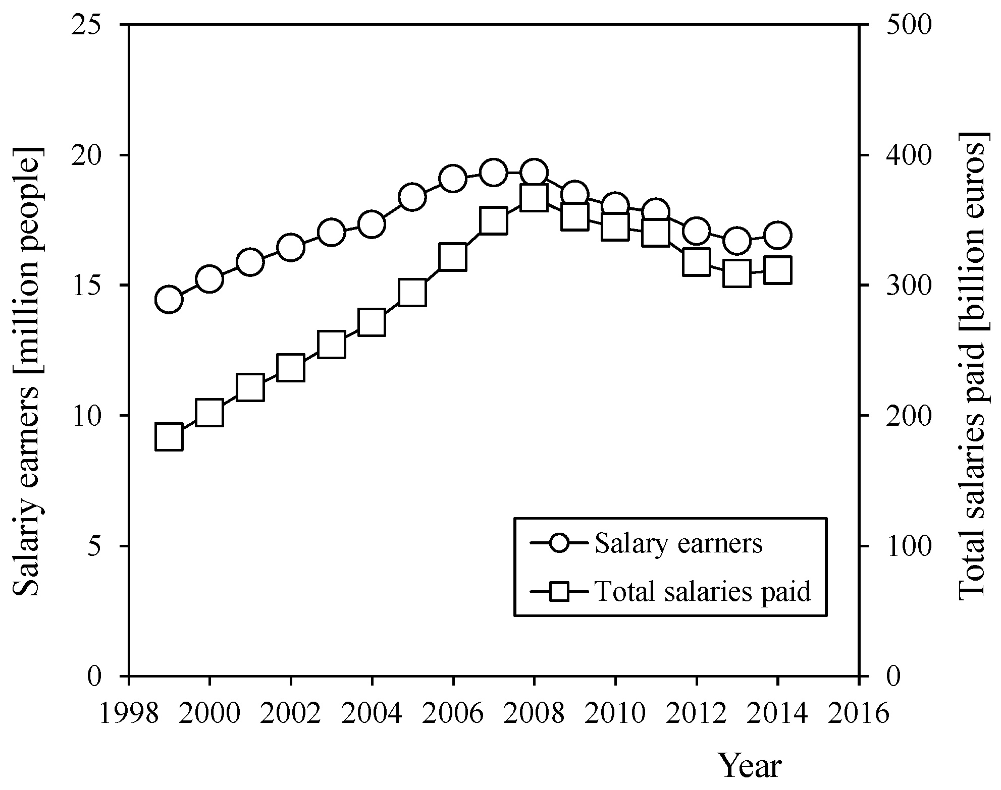
Figure 3.
(Left) Estimated number of salary earners as a function of the non-dimensional salary paid, φ (expressed in multiples of the minimum wage), within the 0.5 minimum wage sub-brackets, which divide the official 5–7.5 and 7.5–10 times the minimum wage brackets, in Spain (2014). The variables corresponding to Equations (3) and (4) in relation to the official 5–7.5 bracket are indicated in the graph. (Right) Salary earners in Spain (2014) as a function of the non-dimensional salary paid, φ. (Official Statistics 2014, see footnote 1)

Figure 4.
Salaries paid (in terms of percentage of the total amount, TSP) in 2014 as a function of the non-dimensional salary paid, φ (expressed in times the minimum wage). The Fréchet distribution has been fitted to the data (Equation (8); λ = 0.479; γ = 8.55; c = 13.6; d = −11.18), together with the Log-Normal (Equation (9); λ = 0.478; a = 1.15; b = 0.658), the Gamma (Equation (10); λ = 0.463; a = 2.856; b = 1.188), the Dagum (Equation (11); λ = 0.490; a = 3.740; b = 4.160; p = 2.287; d = −2.445), and the GB 2 (Equation (12); λ = 0.493; a = 5.218; b = 5.046; ξ = 2.112; η = 0.740; d = −3.532) distributions.
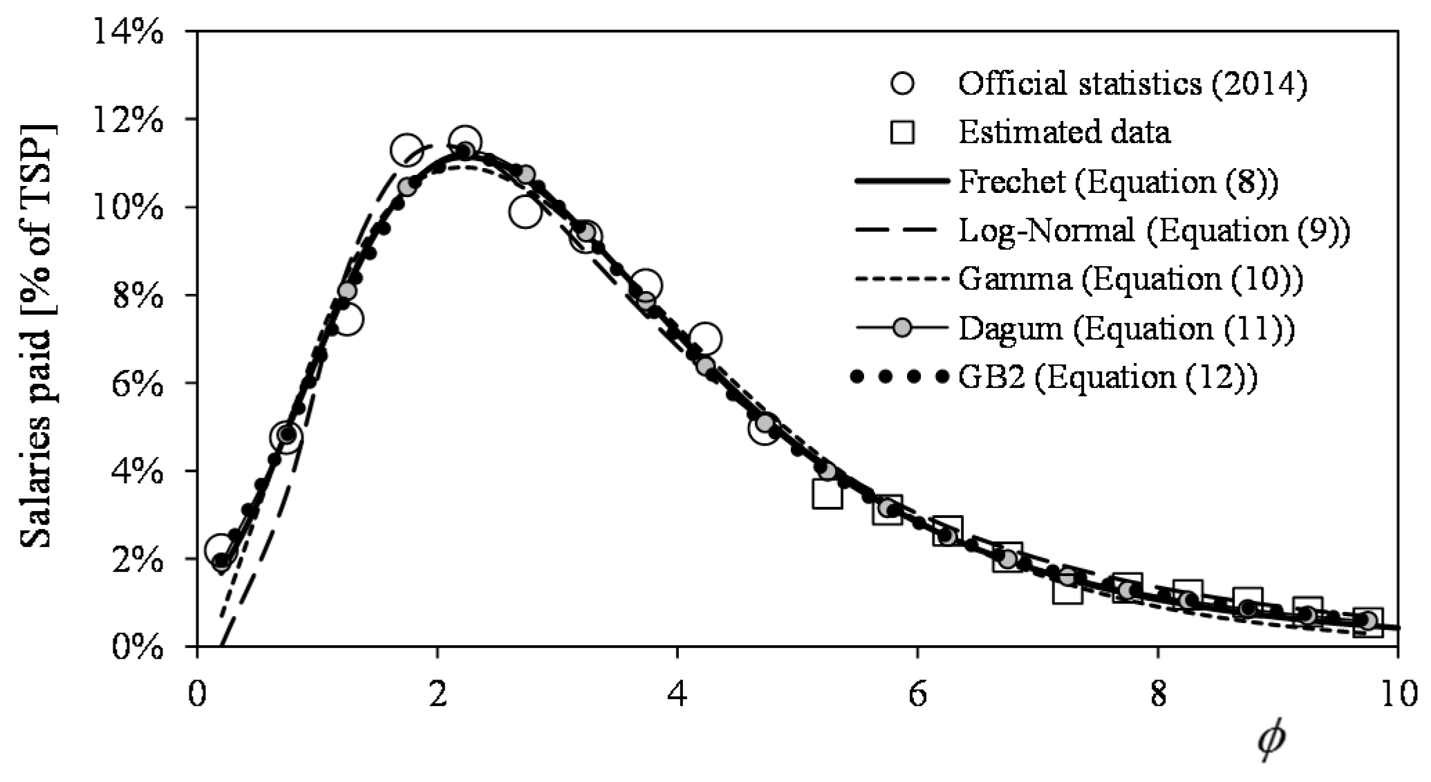
Figure 5.
Evolution of coefficients from Equations (6) and (8), once fitted to the official statistics data (Table 1 and Table 2).
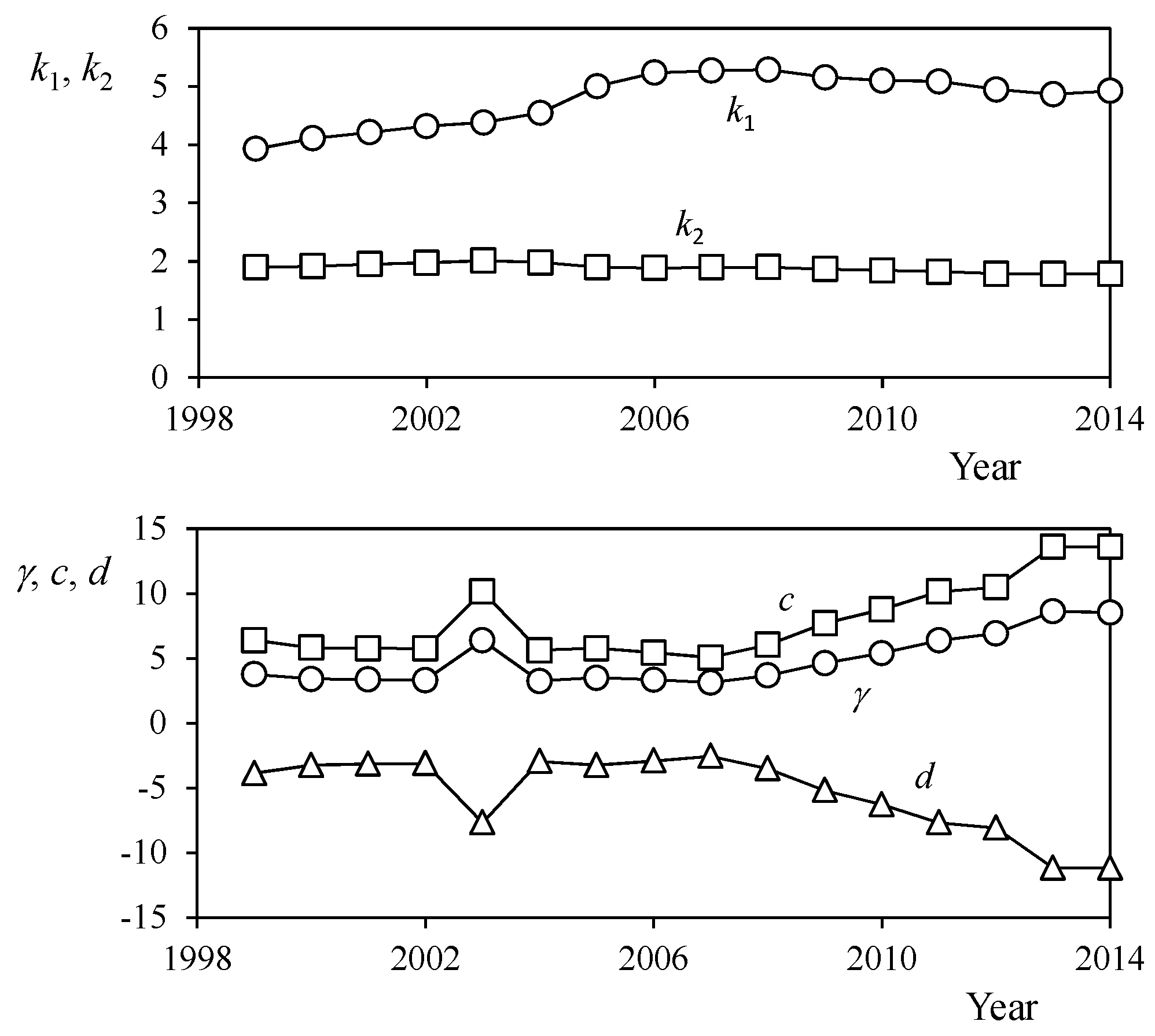
Figure 6.
(Left) RMSE related to Equation (8) fittings to the official statistics data, see Table 2. (Right) Average values of the aforementioned fittings (dashed lines represent the higher and the lower values of that fittings) in relation to the perceived salary, φ (expressed in times the minimum salary). On the right y-axis: averaged error when comparing the fittings and the official statistics data (the standard deviation bars have also been included; the highest levels of the standard deviation have been indicated by dashed ellipses).

Figure 7.
(Left) Evolution from 1999 to 2014 of the of the percentage salary earners within the 0%–30%, 30%–70%, and more than 70% of the total salaries paid brackets; (Right) Yearly variations of the aforementioned the percentage salary earners within the 30%–70% bracket in relation to the variations of the the percentage salary earners within the 0%–30% bracket.
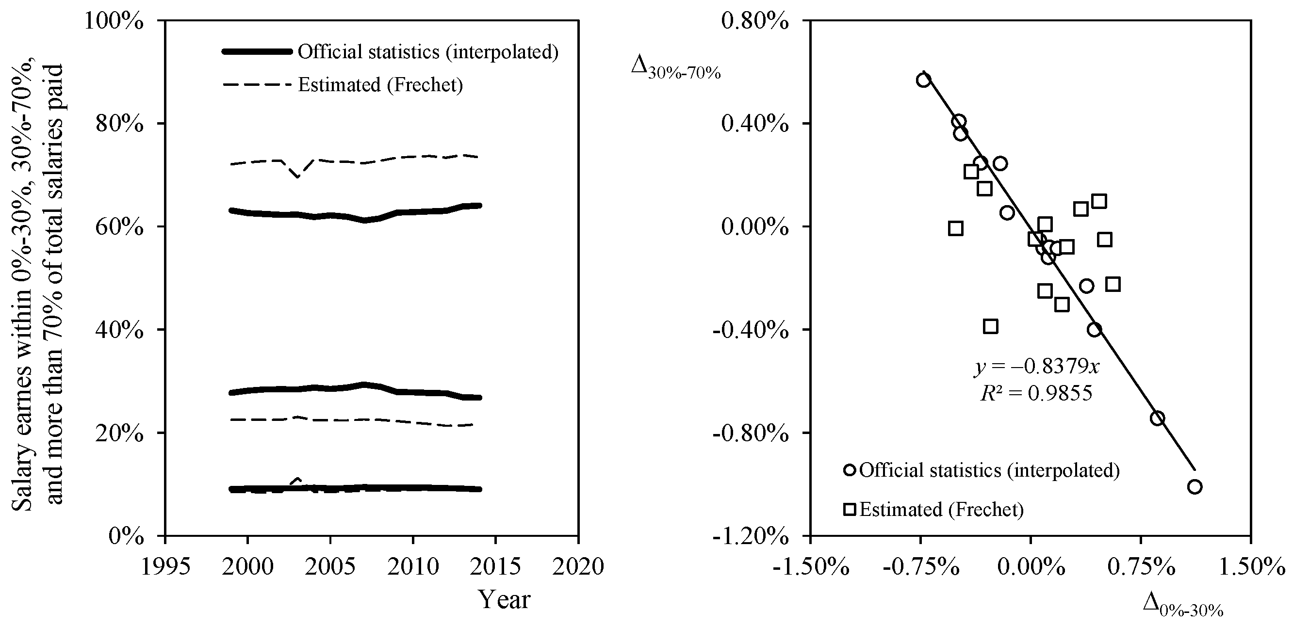
Figure 8.
Evolution from 1999 to 2014 of the Fréchet distribution fittings asymmetry parameter, ψ, (open circles; defined with equation (23)). The calculated skewness of the Fréchet distribution fittings, skw, (open squares), and the evolution of the Gini coefficient (open rhombi) have been also included in the graph.

Figure 9.
Lorenz curves representing the wage distributions in 1999, 2005, and 2013. Percentage of the wages, L(p), perceived by a percentage p of the salaried people in relation to the percentage of the salaried people, p. The dashed straight line corresponds to the theoretical maximum equality level.

Figure 10.
Difference between the Lorenz curves and the theoretical maximum equality level, p – L(p), in relation to the percentage of salaried people, p, in 2007 and 2012 (left). Location of the maximum point on these curves (right).
Figure 10.
Difference between the Lorenz curves and the theoretical maximum equality level, p – L(p), in relation to the percentage of salaried people, p, in 2007 and 2012 (left). Location of the maximum point on these curves (right).

Figure 11.
Evolution from 1999 to 2014 of the salaried people percentage corresponding to the maximum difference between the Lorentz curve applied to the salaries distribution and the theoretical maximum equality level.
Figure 11.
Evolution from 1999 to 2014 of the salaried people percentage corresponding to the maximum difference between the Lorentz curve applied to the salaries distribution and the theoretical maximum equality level.


Table 1.
Salary earners per income bracket in Spain from 1999 to 2014 (expressed in million people). Source: Agencia Tributaria de España.
Table 1.
Salary earners per income bracket in Spain from 1999 to 2014 (expressed in million people). Source: Agencia Tributaria de España.
| Income | 1999 | 2000 | 2001 | 2002 | 2003 | 2004 | 2005 | 2006 | 2007 | 2008 | 2009 | 2010 | 2011 | 2012 | 2013 | 2014 |
|---|---|---|---|---|---|---|---|---|---|---|---|---|---|---|---|---|
| 0 to 0.5 min. wage | 2.784 | 2.774 | 2.795 | 2.833 | 2.911 | 2.851 | 3.232 | 3.286 | 2.988 | 3.090 | 3.405 | 3.420 | 3.466 | 3.494 | 3.642 | 3.695 |
| 0.5 to 1 min. wage | 1.688 | 1.739 | 1.760 | 1.817 | 1.829 | 1.887 | 2.145 | 2.187 | 2.214 | 2.284 | 2.251 | 2.207 | 2.211 | 2.122 | 2.110 | 2.197 |
| 1 to 1.5 min. wage | 1.743 | 1.819 | 1.839 | 1.870 | 1.872 | 1.970 | 2.211 | 2.359 | 2.492 | 2.481 | 2.284 | 2.215 | 2.175 | 2.051 | 1.982 | 2.047 |
| 1.5 to 2 min. wage | 2.182 | 2.341 | 2.388 | 2.440 | 2.418 | 2.583 | 2.824 | 3.010 | 3.169 | 2.966 | 2.678 | 2.592 | 2.500 | 2.417 | 2.224 | 2.220 |
| 2 to 2.5 min. wage | 1.595 | 1.760 | 1.926 | 2.024 | 2.144 | 2.174 | 2.188 | 2.281 | 2.318 | 2.281 | 2.038 | 1.979 | 1.956 | 1.896 | 1.762 | 1.769 |
| 2.5 to 3 min. wage | 1.033 | 1.114 | 1.215 | 1.282 | 1.374 | 1.399 | 1.411 | 1.467 | 1.528 | 1.548 | 1.430 | 1.389 | 1.373 | 1.344 | 1.251 | 1.244 |
| 3 to 3.5 min. wage | 0.799 | 0.848 | 0.899 | 0.950 | 0.982 | 1.013 | 1.035 | 1.081 | 1.109 | 1.122 | 1.048 | 1.059 | 1.073 | 1.017 | 0.984 | 0.990 |
| 3.5 to 4 min. wage | 0.642 | 0.689 | 0.727 | 0.746 | 0.785 | 0.793 | 0.809 | 0.847 | 0.875 | 0.879 | 0.831 | 0.823 | 0.807 | 0.768 | 0.761 | 0.756 |
| 4 to 4.5 min. wage | 0.524 | 0.548 | 0.579 | 0.605 | 0.641 | 0.643 | 0.639 | 0.657 | 0.677 | 0.689 | 0.654 | 0.641 | 0.630 | 0.553 | 0.567 | 0.569 |
| 4.5 to 5 min. wage | 0.374 | 0.417 | 0.454 | 0.484 | 0.521 | 0.522 | 0.480 | 0.491 | 0.511 | 0.521 | 0.498 | 0.456 | 0.419 | 0.342 | 0.357 | 0.361 |
| 5 to 7.5 min. wage | 0.718 | 0.791 | 0.866 | 0.935 | 1.030 | 1.003 | 0.936 | 0.953 | 0.958 | 0.979 | 0.916 | 0.851 | 0.803 | 0.727 | 0.722 | 0.726 |
| 7.5 to 10 min. wage | 0.205 | 0.224 | 0.247 | 0.265 | 0.290 | 0.282 | 0.263 | 0.267 | 0.276 | 0.277 | 0.250 | 0.236 | 0.225 | 0.201 | 0.195 | 0.197 |
| More than 10 min. wage | 0.143 | 0.156 | 0.177 | 0.187 | 0.204 | 0.199 | 0.187 | 0.185 | 0.194 | 0.194 | 0.168 | 0.156 | 0.149 | 0.133 | 0.125 | 0.128 |
| Total amount | 14.431 | 15.220 | 15.871 | 16.438 | 17.001 | 17.321 | 18.360 | 19.070 | 19.309 | 19.311 | 18.452 | 18.025 | 17.788 | 17.063 | 16.682 | 16.899 |
Table 2.
Salaries payed per income bracket in Spain from 1999 to 2014 (expressed in billion euros). Source: Agencia Tributaria de España.
Table 2.
Salaries payed per income bracket in Spain from 1999 to 2014 (expressed in billion euros). Source: Agencia Tributaria de España.
| Income | 1999 | 2000 | 2001 | 2002 | 2003 | 2004 | 2005 | 2006 | 2007 | 2008 | 2009 | 2010 | 2011 | 2012 | 2013 | 2014 |
|---|---|---|---|---|---|---|---|---|---|---|---|---|---|---|---|---|
| 0 to 0.5 min. wage | 3.428 | 3.499 | 3.615 | 3.733 | 3.856 | 4.122 | 4.991 | 5.303 | 5.221 | 5.632 | 6.371 | 6.392 | 6.513 | 6.407 | 6.586 | 6.797 |
| 0.5 to 1 min. wage | 7.363 | 7.746 | 8.002 | 8.424 | 8.659 | 9.420 | 11.542 | 12.440 | 13.320 | 14.420 | 14.684 | 14.571 | 14.789 | 14.203 | 14.216 | 14.791 |
| 1 to 1.5 min. wage | 12.778 | 13.601 | 14.031 | 14.534 | 14.831 | 16.453 | 19.914 | 22.471 | 25.085 | 26.241 | 25.107 | 24.716 | 24.544 | 23.128 | 22.464 | 23.172 |
| 1.5 to 2 min. wage | 22.269 | 24.417 | 25.470 | 26.584 | 26.922 | 30.288 | 35.597 | 39.996 | 44.331 | 43.662 | 40.927 | 40.203 | 39.278 | 37.991 | 35.191 | 35.111 |
| 2 to 2.5 min. wage | 20.731 | 23.326 | 26.059 | 27.944 | 30.219 | 32.280 | 34.993 | 38.500 | 41.291 | 42.758 | 39.756 | 39.181 | 39.223 | 38.002 | 35.558 | 35.704 |
| 2.5 to 3 min. wage | 16.480 | 18.110 | 20.168 | 21.698 | 23.731 | 25.460 | 27.674 | 30.349 | 33.338 | 35.536 | 34.118 | 33.635 | 33.707 | 33.073 | 30.925 | 30.757 |
| 3 to 3.5 min. wage | 15.097 | 16.348 | 17.707 | 19.081 | 20.113 | 21.888 | 24.105 | 26.549 | 28.721 | 30.570 | 29.697 | 30.445 | 31.226 | 29.571 | 28.807 | 28.978 |
| 3.5 to 4 min. wage | 14.007 | 15.329 | 16.516 | 17.279 | 18.533 | 19.749 | 21.738 | 24.008 | 26.151 | 27.623 | 27.164 | 27.292 | 27.099 | 25.768 | 25.710 | 25.547 |
| 4 to 4.5 min. wage | 12.931 | 13.828 | 14.899 | 15.871 | 17.152 | 18.140 | 19.458 | 21.106 | 22.943 | 24.528 | 24.203 | 24.110 | 23.975 | 20.996 | 21.671 | 21.755 |
| 4.5 to 5 min. wage | 10.305 | 11.732 | 13.052 | 14.202 | 15.600 | 16.467 | 16.299 | 17.573 | 19.310 | 20.718 | 20.581 | 19.133 | 17.779 | 14.550 | 15.258 | 15.415 |
| 5 to 7.5 min. wage | 24.948 | 28.028 | 31.311 | 34.474 | 38.690 | 39.767 | 40.058 | 42.975 | 45.575 | 48.938 | 47.509 | 44.870 | 42.974 | 38.942 | 38.911 | 39.099 |
| 7.5 to 10 min. wage | 10.173 | 11.350 | 12.779 | 13.986 | 15.623 | 16.000 | 16.109 | 17.227 | 18.786 | 19.842 | 18.658 | 17.795 | 17.218 | 15.364 | 14.955 | 15.148 |
| More than 10 min. wage | 13.049 | 14.792 | 17.513 | 18.397 | 20.460 | 21.172 | 21.600 | 22.819 | 25.165 | 26.353 | 23.370 | 22.163 | 21.463 | 19.402 | 18.443 | 19.006 |
| Total amount | 183.56 | 202.11 | 221.12 | 236.21 | 254.39 | 271.21 | 294.08 | 321.32 | 349.24 | 366.82 | 352.15 | 344.51 | 339.79 | 317.40 | 308.70 | 311.28 |
Table 3.
Minimum wage (paid yearly) in Spain from 1998 to 2014.
| Year | Minumum Wage [€] | Year | Minumum Wage [€] |
|---|---|---|---|
| 1998 | 5725.02 | 2007 | 7988.4 |
| 1999 | 5828.48 | 2008 | 8400 |
| 2000 | 5947.2 | 2009 | 8736 |
| 2001 | 6068.3 | 2010 | 8866.2 |
| 2002 | 6190.8 | 2011 | 8979.6 |
| 2003 | 6316.8 | 2012 | 8979.6 |
| 2004 | 6659.1 | 2013 | 9034.2 |
| 2005 | 7182 | 2014 | 9034.2 |
| 2006 | 7572.6 |
Table 4.
Coefficients of the mathematical expressions (Equations (6) and (8)) fitted to the salary earners and the salaries paid (Table 1 and Table 2, respectively) from 1999 to 2014. Coefficient k1 is expressed in millions of people; k2, γ, c, d, λ are dimensionless.
| Year | k1 | k2 | γ | c | d | λ |
|---|---|---|---|---|---|---|
| 1999 | 3.93 | 1.89 | 3.78 | 6.40 | −3.86 | 0.488 |
| 2000 | 4.11 | 1.92 | 3.42 | 5.83 | −3.25 | 0.489 |
| 2001 | 4.21 | 1.95 | 3.37 | 5.78 | −3.15 | 0.486 |
| 2002 | 4.32 | 1.97 | 3.32 | 5.76 | −3.10 | 0.488 |
| 2003 | 4.38 | 2.01 | 6.39 | 10.15 | −7.68 | 0.480 |
| 2004 | 4.55 | 1.98 | 3.25 | 5.62 | −2.95 | 0.487 |
| 2005 | 5.01 | 1.90 | 3.51 | 5.78 | −3.24 | 0.484 |
| 2006 | 5.24 | 1.89 | 3.35 | 5.44 | −2.92 | 0.485 |
| 2007 | 5.27 | 1.90 | 3.13 | 5.06 | −2.54 | 0.486 |
| 2008 | 5.29 | 1.90 | 3.68 | 6.04 | −3.51 | 0.485 |
| 2009 | 5.16 | 1.87 | 4.63 | 7.71 | −5.18 | 0.486 |
| 2010 | 5.10 | 1.84 | 5.41 | 8.78 | −6.29 | 0.483 |
| 2011 | 5.09 | 1.82 | 6.39 | 10.15 | −7.68 | 0.480 |
| 2012 | 4.95 | 1.79 | 6.93 | 10.49 | −8.08 | 0.475 |
| 2013 | 4.87 | 1.78 | 8.62 | 13.61 | −11.18 | 0.479 |
| 2014 | 4.93 | 1.78 | 8.55 | 13.60 | −11.18 | 0.479 |
Table 5.
Wage levels, φ30% and φ70%, that indicate 30% and 70% of the total amount of salaries paid and the number of salaries paid (salaried people) within the 0%–30%, 30%–70%, and more than 70% salaries paid brackets from 1999 to 2014. Two different figures are included: ‘calc.’ stands for the figures calculated by interpolating on the official statistical data, whereas ‘est.’ stands for the figures estimated with the fittings of Equations (6) and (8).
| Year | φ30% | φ70% | S0%–30% [%] | S30%–70% [%] | S70%-∞ [%] | |||||
|---|---|---|---|---|---|---|---|---|---|---|
| calc. | est. | calc. | est. | calc. | est. | calc. | est. | calc. | est. | |
| 1999 | 2.04 | 2.27 | 4.50 | 4.72 | 63.1 | 72.1 | 27.8 | 22.5 | 9.1 | 8.5 |
| 2000 | 2.07 | 2.30 | 4.56 | 4.79 | 62.6 | 72.4 | 28.2 | 22.6 | 9.2 | 8.5 |
| 2001 | 2.12 | 2.36 | 4.67 | 4.90 | 62.4 | 72.7 | 28.4 | 22.5 | 9.2 | 8.4 |
| 2002 | 2.14 | 2.38 | 4.71 | 4.93 | 62.3 | 72.8 | 28.5 | 22.5 | 9.3 | 8.5 |
| 2003 | 2.01 | 2.23 | 4.29 | 4.48 | 62.3 | 69.5 | 28.4 | 23.1 | 9.3 | 11.2 |
| 2004 | 2.15 | 2.40 | 4.72 | 4.95 | 61.8 | 73.1 | 28.8 | 22.5 | 9.4 | 8.6 |
| 2005 | 2.05 | 2.29 | 4.50 | 4.73 | 62.2 | 72.5 | 28.5 | 22.5 | 9.2 | 8.6 |
| 2006 | 2.03 | 2.27 | 4.45 | 4.69 | 61.9 | 72.6 | 28.8 | 22.4 | 9.3 | 8.7 |
| 2007 | 2.02 | 2.27 | 4.45 | 4.69 | 61.2 | 72.3 | 29.4 | 22.6 | 9.5 | 8.8 |
| 2008 | 2.04 | 2.28 | 4.46 | 4.69 | 61.6 | 72.8 | 29.0 | 22.5 | 9.5 | 8.8 |
| 2009 | 2.04 | 2.26 | 4.42 | 4.62 | 62.7 | 73.3 | 28.0 | 22.3 | 9.3 | 8.8 |
| 2010 | 2.02 | 2.25 | 4.35 | 4.54 | 62.8 | 73.5 | 27.9 | 22.0 | 9.3 | 8.9 |
| 2011 | 2.01 | 2.23 | 4.29 | 4.48 | 62.9 | 73.6 | 27.7 | 21.7 | 9.3 | 9.0 |
| 2012 | 1.97 | 2.20 | 4.18 | 4.37 | 63.0 | 73.4 | 27.7 | 21.4 | 9.3 | 9.0 |
| 2013 | 1.99 | 2.20 | 4.24 | 4.40 | 63.9 | 73.8 | 26.9 | 21.5 | 9.2 | 8.9 |
| 2014 | 1.98 | 2.19 | 4.24 | 4.40 | 64.1 | 73.4 | 26.8 | 21.7 | 9.1 | 8.8 |
© 2017 by the authors. Licensee MDPI, Basel, Switzerland. This article is an open access article distributed under the terms and conditions of the Creative Commons Attribution (CC BY) license (http://creativecommons.org/licenses/by/4.0/).
Share and Cite
MDPI and ACS Style
Pindado, S.; Pindado, C.; Cubas, J. Fréchet Distribution Applied to Salary Incomes in Spain from 1999 to 2014. An Engineering Approach to Changes in Salaries’ Distribution. Economies 2017, 5, 14. https://doi.org/10.3390/economies5020014
AMA Style
Pindado S, Pindado C, Cubas J. Fréchet Distribution Applied to Salary Incomes in Spain from 1999 to 2014. An Engineering Approach to Changes in Salaries’ Distribution. Economies. 2017; 5(2):14. https://doi.org/10.3390/economies5020014
Chicago/Turabian StylePindado, Santiago, Carlos Pindado, and Javier Cubas. 2017. "Fréchet Distribution Applied to Salary Incomes in Spain from 1999 to 2014. An Engineering Approach to Changes in Salaries’ Distribution" Economies 5, no. 2: 14. https://doi.org/10.3390/economies5020014
Note that from the first issue of 2016, this journal uses article numbers instead of page numbers. See further details here.