
Management of Oil Revenues: Has That of Azerbaijan Been Prudent?


1
Department of World Economy, Baku Engineering University, Baku AZ0101, Azerbaijan
2
Department of Economics, University of Southern California, Los Angeles, CA 90089, USA
3
Department of Statistics, Azerbaijan State University of Economics (UNEC), Baku AZ1001, Azerbaijan
4
Institute for Scientific Research on Economic Reforms, Baku AZ1011, Azerbaijan
*
Author to whom correspondence should be addressed.
Economies 2017, 5(2), 19; https://doi.org/10.3390/economies5020019
Submission received: 20 December 2016
/
Revised: 23 May 2017
/
Accepted: 31 May 2017
/
Published: 12 June 2017
(This article belongs to the Special Issue The Impact of Natural Resources on Economic Development in an Era of Globalization)
Abstract
:To help explain the common failure of oil or other natural resource exporting countries to diversify into industry, it has been common to trace this failure to real exchange rate appreciation. This has also been done in Azerbaijan. However, because Azerbaijan has devoted so much of its oil revenues to government investment, Azerbaijan provides a suitable case for examining an alternative link through government investment. This study applies the ARDL cointegration method to quarterly time series data on oil prices, government capital formation, non-oil exports and non-oil GDP to estimate the long run relationships linking oil prices to government investment expenditures and further to generation of non-oil GDP. The results show that despite the massive government investment expenditures, extremely little non-oil production of the tradable type has been generated, calling attention to the need for policy reform.
Keywords:
oil windfall gains; government capital expenditures; non-oil diversification; industrial policy; sovereign wealth funds; AzerbaijanJEL Classification:
Q01; Q32; Q43; H54; L52; O23; O25; O531. Introduction
Oil production data dates from 1846 and shows that during its first oil boom (1885–1920) Azerbaijan was not only very innovative in its drilling and lifting processes but was usually producing about half of the world’s oil (Balayev 1969; Mir-Babayev and Fuchs 1999; Pomfret 2006, 2011). Hence, it is clear that Azerbaijan has been a large oil producing country for some time. During the time that it was part of the Soviet Union from 1920 to 1991, it became somewhat less innovative and less important as the industry was taken out of private hands and monopolized. During that time, its oil revenues were accrued mainly to the central government of the USSR. However, since the time of Azerbaijan’s independence in late 1991, its oil revenues have increased and their use has come under the management of the Azerbaijan state. To its credit, Azerbaijan has undertaken four significant initiatives toward suitable management of its oil.
The first such initiative was to sign the well-known “Contract of the Century”, a bundle of numerous Production Sharing Agreements (PSA) in 1994 with 11 major oil companies for the Azeri-Chirag-Guneshli oilfields.1 This led to some $60 billion of Foreign Direct Investment (FDI) and sharp increases in Azerbaijan’s oil production since 1997 (Ciaretta and Nasirov 2012, p. 285). The second was taken in 1999 when it created a special oil fund, the State Oil Fund of the Republic of Azerbaijan (SOFAZ). Its purpose was to accumulate savings from its oil revenues for the purposes of macroeconomic stabilization, saving for future generations and investment in important national development projects. Third, soon after that, it decided to join the Extractive Industries Transparency Initiative (EITI), an international NGO designed to increase transparency in the flow of funds between the extractors of the oil or minerals and the recipients (governments or national oil companies) and thereby to reduce the likelihood of missing funds and corruption through the adoption of best practice standards2. In 2004, Azerbaijan undertook a fourth important initiative, by initiating a fiscal rule linking the oil price to the percentage of oil revenues which would be automatically syphoned off from its budget to SOFAZ3.
As demonstrated in Section 2 (to follow), Azerbaijan’s dependence on oil has rather steadily increased over its new oil boom period, at least up to the dramatic fall in oil prices beginning in late 2014. Yet, Azerbaijan’s oil and gas reserves will not last forever, and indeed according to the World Bank (2011) Azerbaijan’s oil production (but not its gas) will decline by no later than 2024. When its oil and gas resources begin to run out, of course, the main sources of exports and government revenues will have to shift to the non-oil sectors and especially manufacturing. Accomplishing this will require building up the appropriate infrastructure and raising the share of manufacturing in GDP well above the 5.5% average maintained over the period 2004-2015 shown in Table 1.
In recognition of its continuing dearth of industrial development, in 2014 Azerbaijan announced a five year state industrial development program.4 Yet, especially after the subsequent sharp fall in oil prices (which many expect to continue for some time), the feasibility of this program is already in jeopardy, thereby motivating our investigation into the research question: “Where and why has Azerbaijan been falling short in allocating its prodigious oil windfall gains since 2004 in fostering development of its non-oil GDP?” While the four aforementioned initiatives that Azerbaijan has taken to mitigate the volatility and other problems associated with oil have been impressive and compare favorably to most other oil exporters, its achievements in terms of industrial diversification have been much less impressive. Many analysts of the Azerbaijan economy, e.g., Ahmadov et al. 2011; Pomfret 2012; Aslanli 2015, have already come to a similar conclusion. What they have not done, however, is to identify the specific sources of, or mechanisms leading to, incomplete diversification. In particular, to accomplish this we utilize quarterly data on oil prices, government investment, non-oil GDP and non-oil exports to identify the significant long term relationship between oil prices and government investment expenditures, on the one hand, and non-oil GDP and exports on the other. The magnitudes of these estimates of the long run relationships reveal very clearly the sources of the serious shortfalls in inducing growth of non- oil GDPandexports.
Several important reasons for the promotion of the non-oil sector (and manufacturing in particular) in oil-exporting countries like Azerbaijan have been given in the literature. One of these is that these sectors, unlike the oil sector, exert multiplier effects on job creation. Note that in Azerbaijan, the oil sector by itself has never employed as much as 1 percent of the total labor force. Another is that, unlike the oil sector, these sectors can exert important backward and forward linkages that can stimulate investment and growth throughout the economy. Also, manufacturing often serves as the focal point for R & D and innovation in the economy, an important contributor to technological change. Yet, data from the United Nations Industrial Development Organization (UNIDO) shows that, in Azerbaijan, value-added manufacturing constitutes only about 5% of GDP. Considering that 41.9% of the country’s manufacturing consists of refined petroleum products, coke and nuclear fuel, it is not surprising that Azerbaijan is ranked 100th out of the 144 countries ranked in on UNIDO’s Competitive Industrial Performance Index5 and that Azerbaijan’s share in world value-added manufacturing in 2005, 2009 and 2011 was only 0.01% (UNIDO 2011, 2013). This paper identifies a major but heretofore largely overlooked contributor to the rather disappointing extent of industrial and export diversification.
The Head of the State Statistical Committee of the Republic of Azerbaijan, Arif Aliyev, announced in late 2013, that the total investment taking place in social and infrastructure projects in Azerbaijan during the period 2003–2013 equaled about $132 billion, some 51% of which was financed from domestic sources, mostly government investment expenditures (Trend News Agency 2013). Moreover, between 2001 and 2016, 83 billion dollars was transferred from the state oil fund to the budget. With such a large share of oil revenues going to the budget and from there to government capital expenditures, it again raises the aforementioned question: How effective has the allocation of government capital expenditures been in fostering non-oil GDP and exports? Answering that question is the main objective of this paper.
Unless major new energy reserves are discovered, by 2024 Azerbaijan will no longer be a resource-rich country. Even just seven years from now it is believed that the Azerbaijan economy will be much in need of manufacturing to generate productive jobs sufficient to sustain anything close to full employment. Because of this, it is indeed high time for Azerbaijani policymakers to find out how to take better advantage of its oil and gas revenues. In this study, we find that there is a strong relationship between the real oil price and real government capital expenditures but that these expenditures have done little to achieve diversification and non-oil tradable goods. As a result, volatility remains high. Indeed, since oil prices began falling in late 2014, Azerbaijan has suffered large fiscal deficits, a sharp acceleration in inflation, rising national debt, two currency devaluations, bank failures, and in 2016 a negative growth rate.6
As will be pointed out in Section 3, the most common explanation for de-industrialization following an oil boom is currency appreciation as in the Dutch disease models. In the case of Azerbaijan, however, we argue that this cannot be the only explanation since the industrial sectors had already tremendously deteriorated during and after the transition to independence from the Soviet Union and that this happened despite massive government capital expenditures which normally would have been expected to boost economic growth.
The main contributions of this paper, therefore, are: (1) to highlight the experience of an understudied, long time major oil country, Azerbaijan, (2) to take advantage of more recent quarterly data for Azerbaijan that allows us to construct and apply a considerably longer time series in identifying long-term effects of oil prices than utilized in previous studies of this country, (3) to demonstrate the applicability of this alternative mechanism ,i.e., the link between the oil price, government capital expenditures and non-oil GDP and exports, in explaining Azerbaijan’s lack of success in industrial diversification, and (4) to demonstrate the method-robustness of the results obtained with respect to different cointegration methods. Our main empirical finding is that, while there is an extremely tight positive relation between oil prices and government capital expenditures, these expenditures have generated only a modest increase in non-oil GDP and a fall in non-oil exports. These findings lead us to some potentially important and timely policy recommendations.
The remainder of the paper is organized as follows. In the next section, Section 2, we provide a more comprehensive description of Azerbaijan’s experience in managing its oil revenues, beginning with its second oil boom lasting through 2013 but followed by the current period of low oil prices. Our focus is on the relation between oil prices and non-oil industrial production. Section 3 presents a brief review of relevant literature on both the fiscal management problem in oil countries in general and its application to Azerbaijan in particular. In Section 4 we present the data and methods utilized, as well as the empirical findings, including a discussion of the results and related tests. Finally, in Section 5 we utilize these findings to draw some important policy recommendations.
2. Further Background on Azeri Oil, Its Management, Accomplishments and Problems
As Hasanov (2013) and others have suggested, Azerbaijan’s transition after the collapse of the Soviet Union was very painful indeed. It displayed symptoms similar to those of Russia and other Former Soviet Union countries. Its heavy reliance on central government subsidies for its manufacturing sectors rendered these industries uncompetitive after the breakup of the USSR. Once they faced competition in free world markets beginning in 1991, these sectors collapsed as shown in Figure 1. Since, as indicated above, the industrial output index (in real terms) in Figure 1 includes at least part of the hydrocarbon sector itself, the real decline in the non-oil manufacturing sector was even greater than the index shows. Azerbaijan also suffered enormous losses of life and property in its war with Armenia (1992-4). Indeed, as shown in Table 1, the share of value-added manufacturing in Azerbaijan’s GDP in 2005 was still only 7.1% and fell to 4.2% in 2011. (See also UNIDO 2013, p. 196). Unfortunately, there does not seem to be a link between the series on industrial output through 2001 at constant price in Figure 1 and the constant price data for manufacturing available on the website of the State Statistical Committee of the Azerbaijan Republic beginning in 2004. Even if, as it would appear, value-added manufacturing at constant prices may have tripled between 2004 and 2015, this would only have managed to bring the level of industrial production in real terms up to its 1991 level.
Yet, as a result of Azerbaijan’s success in inducing eleven oil companies (led by BP) to sign the aforementioned Production Sharing Agreements (PSA) with the government in 1994, FDI was plowed into the oil sector and the infrastructural investments needed to develop both its production and export capabilities. As a result, after 2000 substantial increases in oil production were realized. Thanks also to the rapidly increasing oil prices after 2000, and the completion of the Baku-Tbilsi-Ceyhan pipeline in 2005, the share of oil rents in GDP averaged nearly 50% over the period 2000–2013. These shares were among the highest in the world (the only other countries with such high shares over this period being Republic of Congo, Equatorial Guinea, Iraq, Kuwait and Libya) and were well above those of both Saudi Arabia and Venezuela (according to World Bank data (World Bank 2011) and World Bank Indicators). As a result, the impacts of oil on the Azerbaijan economy became extremely powerful, inducing a true oil boom by about 2003, leading to real GDP growth of 10% in 2004, another 26% in 2005, 34.5% in 2006 and 25% in 2007, clearly demonstrating a close link between oil and the overall economy (Hasanov and Huseynov 2013). As indicated in Table 1, at the height of the oil boom in 2007, the mining sector (including oil and gas) constituted over 57% of GDP. Bildirici and Kayıkçı (2013) showed oil production and revenues to be very tightly linked to GDP (not only in Azerbaijan but also in the other oil-exporting Eurasian countries) to the extent that a 1 percent increase in oil production would increase GDP by about 1%.
Even though the growth rates of oil production and GDP have slowed down since 2007, the levels have stayed high and as a result the shares of oil rents in GDP and oil and gas exports in total exports remained extremely high until 2013. Oil and gas exports and revenues are likely to continue for some time, offering further potential for growth of Azerbaijan’s economy if these revenues can be managed well. Indeed, the World Bank (2009), p. 28, estimated the net present value of Azerbaijan oil and gas revenues to be realized only between 2008 and 2024 to be 198 billion USD (in 2007 prices). See also The BP Statistical Review of World Energy 2014 (BP: 2015).
Nevertheless, as shown in Table 2 below and in more detail by Aslanli (2015) and Pomfret (2011), despite both SOFAZ and the fiscal rule, government consumption expenditures, much of them financed by transfers to the State Budget from SOFAZ, rose sharply. In real terms these expenditures increased seven-fold between 2004 and 2015. (See also Ciaretta and Nasirov 2012, p. 283).
Additional details on the role of SOFAZ in the State Budget can be seen in Table 2. The SOFAZ revenues in the table include not only oil revenues but also other revenues gained by managing the oil fund’s assets, such as transit fees, bonus payments and so on. “Profit Oil” in the table represents the revenues from the Oil and Gas Production Sharing Agreements (PSAs). While early in the oil boom (in 2005), the share of the SOFAZ transfers in State Budget Revenues was only 7%, it rose to an average of well over 50% between 2009 and 2015. In 2015, moreover, the share of transfers to the State Budget from SOFAZ, exceeded 100% of SOFAZ revenues. This is despite the fact that corporate income taxes of the State Oil Company of the Azerbaijan Republic (SOCAR) and multinational oil companies are paid directly to the state budget (Ciaretta and Nasirov 2012, p. 284).
Some examples of what can happen to countries, which do not diversify sufficiently away from the energy sector itself, were provided by Damette and Seghir (2013). They showed that Egypt and Indonesia, though mindful of the need to diversify away from their energy sector, did so by heavily promoting energy-intensive industries, but in the process so drastically increasing local demand for energy as to convert these countries from being substantial energy exporters to being net energy importers. While that has not happened in Azerbaijan, its overall economic dependence on the oil sector has increased, at least until the sharp fall in oil prices since June 2014. According to data taken from the National Accounts of Azerbaijan and presented in Table 1, the share of Mining and Quarrying in GDP (including oil and gas) increased sharply to 57.1% of GDP by 2007 when oil prices were especially high, before leveling off and falling to 37% in 2014 and 28.8% in 2015 following the sharp reduction in oil prices.
Although by its vagueness and lack of enforcement, Azerbaijan’s fiscal rule falls far short of that of Norway7, it is one of the few fiscal rules of any kind adopted by any non-OECD oil exporter. Between 2001:Q2 and 2014:Q1, 105 billion dollars had been accumulated in SOFAZ. This was facilitated by the fact that Azerbaijan benefitted from getting its oil developed and producing at high levels quite early (relative to its Central Asian neighbors) while oil prices remained high (prior to 2008). Thanks to continuing high oil rents from 2008 to April 1, 2014, moreover, SOFAZ assets grew from $5 billion to $36.6 billion, though, as noted by Pomfret (2011, 2012) not by as much as Kazakhstan. Because of the falling oil prices, and the continuing need to finance the rapidly rising government expenditures, by 1 January 2017 SOFAZ assets had fallen slightly to $33.2 billion8.
From Table 3, moreover, one can see rather clearly that its expenditures on non-oil goods and services are being financed by oil revenues and that, even in the most recent years, the contribution of non-oil industrial sectors to the state budget is not enough to reduce the non-oil primary balance below 30%. Hence, it is amply clear that, despite the intent in creating SOFAZ, dependency of the state budget on oil revenues is actually very high. Table 3 also makes clear that the promotion of non-oil exports and GDP must be the means of developing a strong non-oil tax base. For long term sustainable development, all these components will have to come into play. Yet, even now the shares of manufacturing and non-oil production in GDP and exports in Azerbaijan are much smaller than those in Netherlands, Norway and even Indonesia. As Dülger et al. (2013) pointed out, this is likely to make it more difficult for manufacturing and the rest of the non-oil sector to make up for oil revenues as an alternative source of finance and needed macroeconomic and fiscal stability when in the not- too- distant future, oil revenues will start to decline.
Although prior to 2004, Azerbaijan did not have the funds to promote industrial development and reverse its long term decline in that respect, from the oil boom to the present time it had an excellent opportunity to do so. Yet, Table 3 demonstrates very clearly the country’s still continuing excessive dependence of the state budget on oil revenues and it’s continuing high non-oil budget deficit as a percentage of non-oil GDP. Indeed, it also shows the unusually high share of government investment in total investment of Azerbaijan since 2007, indicative of its enormous potential for bringing explosive growth to its non-oil GDP and exports.
3. Literature Review
Before going on to our own search for an answer to our research question and to demonstrating the contribution of the present study, we deem it important to review some relevant literature.
There is by now an enormous literature on the Dutch disease effects of oil, emphasizing that high prices of a country’s oil exports can bring about decline in its tradable goods sector through the appreciation of the country’s real exchange rate (Corden 1984). While this is likely to be a more serious concern for developing countries with lesser ability to engage in efficient monetary and fiscal policies and other means of preventing adverse effects on the structure of industry, Dissou (2010) has shown that it also is a common result in developed countries like Canada. Aye et al. (2014), among many others, have shown that adverse effects on tradable goods can occur even if the country is an exporter, not of oil, but rather of minerals and other primary products which could have similar effects on the real exchange rate.
More specifically, based on a sample of 10 energy-exporting countries, Dauvin (2014) finds that a 10% increase in the energy price of such a country brings about a 2.5% appreciation of its currency. Dülger et al. (2013), in turn, pointed to the role of currency appreciation in the decline of its manufacturing sector and the rise of mostly non-tradable services. In a related study for Kazakhstan, Azhgaliyeva (2014) shows that the real value of oil production raises real government expenditures but that the country’s national oil fund mitigates that unwanted effect on real exchange rate appreciation to some extent. In any case, the adverse effects of oil booms on non-oil industrial production coming from currency appreciation can be offset by a sufficiently strong link through government investment in industry.
When it comes to oil exporting developing and transition countries in general, the examination of effects of oil and oil prices has spread considerably beyond the Dutch disease effects on exchange rates to a wide variety of other variables. Among the common findings in various other countries are positive effects of oil revenues on government consumption expenditures, the government wage bill, fuel and housing subsidies and military spending, and negative effects on the non-oil economy. (See, e.g., Farzanegan and Markwardt (2009); Farzanegan (2011); Esmani and Adipour (2012) on Iran, Dizaji (2014) on MENA countries, Bhattacharya and Blake (2010) on Nigeria, Iwayemi and Fowowe (2011) on Russia, Dülger et al. (2013) on Kazakhstan and both Arezki and Ismail (2013) and El Anshasy and Bradley (2012) on a larger number of oil exporting countries). Many of these studies identify the ability to deal with volatility in their government revenues as a major weakness of oil rich developing countries.
Beginning with the studies of Hamilton and Clemens (1999) and Hamilton and Atkinson (2006), identified as one of the most plausible explanations by Torvik (2009) and Boos and Holm-Muller (2013), is the thesis that an important source of the oil curse on development is its adverse effect on “genuine savings”. This is derived from the fact that oil revenues come about by selling off natural resources, thus lowering the natural capital stock. Unless this resource depletion is offset by sufficient investment in human capital and physical capital, or net financial investment abroad, net national savings (identified as Adjusted Net Saving in the World Bank’s data set related to World Bank 2011, will be substantially reduced, often making it negative.9
In quite a few of the contributions to the more general literature on natural resource exporting countries, the blame for adverse effects of positive oil price shocks is traced even further back to weak institutions, either weak political systems that allow incumbent political leaders to retain inefficient and weak institutions, or directly to the weak institutions themselves (especially weak fiscal institutions or the absence of rule of law and of property rights) (See, for example, Mehlum et al. 2006a, 2006b; Arezki and van der Ploeg 2007; Collier and Hoeffler 2009; Torvik 2009; van der Ploeg 2011; Boos and Holm-Muller 2013; Elbadawi and Soto 2016; and Selim and Zaki 2016).
Yet, many fewer studies include Azerbaijan in their coverage. One exception is the aforementioned study of Arezki and Ismail (2013) since it included Azerbaijan among the 32 oil-exporting countries in its panel data analysis. This study showed that current government spending tends to rise when oil prices rise but not to decrease when oil prices go down, the latter being a good sign in terms of limiting the extent of procyclicality typical of most oil exporters. On the other hand, in the case of government capital expenditures, they showed that there is considerable procyclicality in its effects but they did not relate this to the industrial structure or industrial diversification of these countries. Also they detected an interesting asymmetry in the effects of the two different types of expenditures on the real effective exchange rate, namely government current expenditures bringing about appreciation of that rate but government capital expenditures bringing about depreciation in that rate. They attribute this difference to differences in the input content between the two types of spending, i.e., import-intensive in the case of capital spending and domestic goods-intensive in the case of current spending. Once again, therefore this calls attention to the importance of government investment based on oil revenues.10
Again, and specific to Azerbaijan, Hasanov and Huseynov (2013) found that a 1% real exchange rate appreciation generates a 0.61% decline in the output of its non-oil tradable sectors in the long run, and a 3.21% decline in the short run. Their data, however, was limited to the 2000–2007 period, capturing the effect of only about three years of the oil boom. Although that study did use techniques to reduce the small sample bias, since our study extends the duration of time series up until to 2013 (just a few months before the sharp fall in oil prices and the end of the boom, this gives us a better opportunity to more fully capture the effects of oil boom on the Azerbaijan economy. Earlier, Hasanov (2010) had used an ARDL Error Correction Model and the Johansen Co-integration approach somewhat similar to that we use below for that same 2000–2007 period, to show that a 1% increase in the real oil price leads to a 0.7% increase in the real effective exchange rate of its currency, the manat, suggesting that the decline in non-oil output may have been due to the appreciation of the manat. More recently, however, Hasanov (2013), again with data only for the 2000–2007 period, showed that the rise in the real value of the manat may have been more attributable to the substantial FDI inflows into Azerbaijan than to the higher oil prices. These last several studies further underscore the importance of examining the link from oil prices and revenues to government investment and then to non-oil output instead of through the real exchange rate or the lowering of “genuine” savings rates.11
The link between oil prices and non-oil manufacturing production that we investigate here is one going from oil prices to government capital expenditures and thereby to non-oil manufacturing. This could certainly be positive and thereby act as an offset to the other negative effects. However, if the state capital expenditures flow mainly into infrastructure most useful to non-tradable sectors such as construction and transportation as suggested by the sharply increasing shares of these sectors on aggregate value added shown in Table 1, this effect could also be negative. We believe that this latter negative effect would be the most likely outcome, especially considering the limited absorptive capacity of the Azerbaijan domestic economy. When absorptive capacity is low, government capital expenditures are likely to be much more effective in increasing non-oil services output than manufacturing. To be successful, public procurement policy should be designed in tandem with improving efficiency of the capital expenditures and the ability to absorb them. As Ross (2012) put it,
“Investment is critical, but it cannot be done all at once. Economies have a limited ability to absorb new investments, which are typically constrained by diminishing returns. For instance, if a government tries to build too much infrastructure too quickly, it will lead to poor planning, lax oversight, and shoddy construction at inflated prices”
An important objective of the empirical analysis in the following section is to test the validity of the above hypothesis that the net effect of government capital expenditures on manufacturing is very modest and an important contributor to Azerbaijan’s very limited industrial development and diversification. In doing so it is extremely important to extend the statistical analysis concerning the various effects of oil in Azerbaijan well beyond 2007, the last year covered in the aforementioned studies. Note also that this link is not part of the received literature on the effects of oil price increases in oil exporting countries.
Given the realities of the economics of oil production there are typically substantial costs of adjusting oil output in the short run, when oil prices rise, oil revenues must also rise in some cases quite sharply. Therefore, with oil production constant, in a country where oil revenues accrue to the government, the rising oil price can be expected to raise government revenues rise even in the short run (and in proportion to the rise in oil prices). Unless, there is an unusually strong fiscal rule pulling such increased revenues out of the budget and into, e.g., a sovereign wealth fund, government revenues will increase and likely to induce government expenditures. Typically, since government consumption expenditures are aimed at providing schooling, health, and security outcomes which do not vary sharply over time, one should expect that these increased revenues would go primarily into government capital expenditures for infrastructure of various kinds for longer term growth and diversification purposes, not into additional government consumption expenditures which could be wasteful. This pattern is not only expected but also the efficient way to help avoid the oil curse. In due course, these government capital expenditures would be expected to increase non-oil GDP and especially non-oil exports. The latter would be especially important for a country like Azerbaijan which is gradually approaching a time in which it will be running out of oil.
There can of course be problems of allocative efficiency and implementation which would prevent the capital expenditures from being converted into sizable increases in non-oil GDP and the non-oil exports that will help the country cope with eventual losses in government revenues. It is this possible shortcoming that our empirical approach is designed to detect and indeed since that is detected we hope that it will induce future researchers in resource-rich countries to broaden their approach to the oil curse phenomenon.
4. Data and Methods Used
We begin our econometric investigation into the apparent substantial shortcomings in Azerbaijan’s efforts to convert high oil prices and revenues into investment in manufacturing and thereby development of industrial tradables by returning to some of the other post- 2004 data on sectorial shares in GDP presented in Table 1, all measured at current prices. In addition to the failure of manufacturing to get back even in 2015 to its 7.1% share of GDP registered in 2005, the same can be said about agriculture. Its share in 2015 was still more than 3% below its share in 2005. On the other hand, witness the dramatic increases in the GDP shares of all the more service- oriented non-tradables. Utilities increased from 0.9% of GDP in 2005 to 2.4% in 2015, Construction from 9.8% in 2005 to 13.2% in 2015, Trade, Transportation, Accommodation and Food Services from 12.9% of GDP in 2005 to 19.8% in 2015. There were sharp increases in each of the other three service industries as well, i.e., Finance and Technical Services, Public Administration and Other Services, which collectively rose from 13.6% of GDP in 2005 to 23.1% in 2015.
While these trends are indicative of very incomplete success in industrial diversification, they do not get at the hypothesized links between oil prices and government capital expenditures and thereby to non-oil GDP and exports that is the focus of this paper. We turn next, therefore, to the data used in our empirical analysis in Section A, to the methods of estimation in Section B and to the resulting estimates in Section C. Our purpose in this is to trace out the long-run relationships between each pair of linked variables, mostly based on data in constant prices. We deliberately do not attempt to demonstrate causality, in part because we suspect that in most cases the causality is likely to be two-way. However, what we do want to establish is the direction and magnitude of each long-term relationship.
4.1. Data and Its Sources
To facilitate the investigation of long-term relationships despite the fact that the relevant data covers only a little over a single decade, the data used in estimating the different models presented below is that available on a quarterly basis extending from the first quarter of 2000 until the end of 2013. The definitions and sources of each of the data series utilized are as follows:
Oil price (OP) the Brent oil price per barrel in terms of US dollars. Source: US Energy Information Administration. The data was converted to real terms using US CPI retrieved from the FRED Economic Data. Base year is 2005.
Government capital expenditures (govcap) in million manats (Azerbaijan national currency) at constant 2005 prices. Source: State Development Indicators Bulletin, published by the The State Statistical Committee of the Republic of Azerbaijan.
Non-oil export (noex) at constant prices of 2005. Source: Central Bank of Azerbaijan.
Real non-oil gross domestic product (gdpno) at constant prices of 2005. Source: Central Bank of Azerbaijan.
To consider the effect of the late 2008 Financial crisis we used the dummy variable 2008Q4 in some models, d2008Q4 = 1 for the last quarter of 2008 and 0 otherwise.
We use centered seasonal dummies to capture the effect of seasonality on the variables under study. For example, dcs1 is 0.75 for the 1st quarter dummy and −0.25 for the remaining three quarter dummies.
Note that in our estimations all variables are measured in log terms.
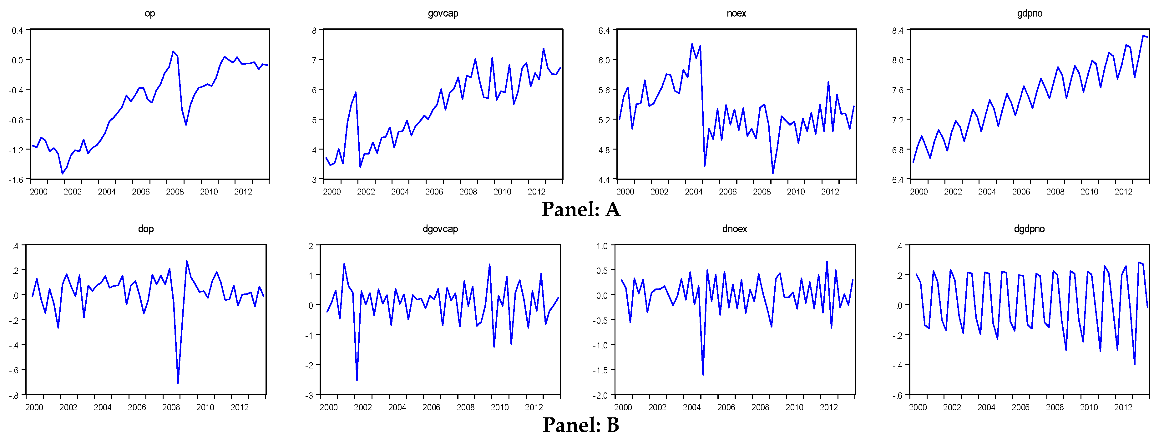
Panel A of Figure 2 shows rather clearly that the oil price, government capital expenditures and real non-oil GDP all increased during the period under study, at least up until 2011. Non-oil exports also rose prior to 2005, but declined sharply thereafter. Panel B of Figure 2 shows the remarkably high volatility in the growth rates from one quarter to the next in each of these series. The descriptive statistics on these variables are given in Table 4. The high values of their coefficients of variation in the last column of that table also provide evidence on the volatility of all four variables and again show that government capital expenditures were considerably more volatile than any of the other variables over the period under study.
4.2. Methodology
4.2.1. Models to be Estimated
To investigate this link between oil prices and diversification away from oil, we estimate three different models: (1) a model relating oil prices (op) to government capital expenditures (govcap), (2) a model relating government capital expenditures (govcap) to non-oil exports (noex), and (3) a model relating government capital expenditures (govcap) to non-oil gdp (gdpno).
4.2.2. The Unit Root Test
First, the order of integration of the variables is examined by means of a Unit Root (UR) test, employing the Augmented Dickey-Fuller test (ADF) of Dickey and Fuller (1981). The test maintains the null hypothesis of non-stationarity of a given time series. Then, once this test has been passed, and concluded that the variables of interest have the same order of integration (smaller than 2) we then employ each of the following three co-integration tests.
4.2.3. The Johansen Cointegration Method
The first co-integration test employed is that of Johansen (1988) and Johansen and Juselius (1990) and is based on the following full information maximum likelihood estimation of a Vector Error Correction Model (VECM):
where, yt is a (n × 1) vector of the n variables of interest, µ is a (n × 1) vector of constants, Г represents a (n × (k − 1)) matrix of short-run coefficients, εt denotes a (n × 1) vector of white noise residuals, and П is a (n × n) coefficient matrix. If the matrix П has reduced rank (0 < r < n), it can be split into a (n × r) matrix of loading coefficients α, and a (n × r) matrix of cointegrating vectors β. The former, matrix Г, shows the importance of the co-integration relationships in the individual equations of the system and the speed of adjustment to disequilibrium. On the other hand, the latter (matrix П) represents the long-term equilibrium relationship, so that . Testing for cointegration, using Johansen’s reduced rank regression approach, centers on estimating the matrix П in unrestricted form, and then testing whether the restriction implied by the reduced rank of П can be rejected. Max Eigen Value and Trace test statistics are used to test for non-zero characteristic roots. If a given variable is statistically significant, it implies that the null hypothesis of corresponding β = zero can be rejected, while stationarity or trend stationarity of a variable assumes that a restriction on long-run coefficients cannot be rejected.
4.2.4. Fully Modified Ordinary Least Squares Method (FMOLS)
Next, we use the FMOLS method, developed by Phillips and Hansen (1990). This method has the advantage of eliminating the sample bias and correcting for endogeneity resulting from co-integrated relationships and serial correlation effects (Narayan and Narayan 2004). (See Phillips and Hansen (1990) for a detailed mathematical derivation of the model).
4.2.5. Dynamic Ordinary Least Squares Method (DOLS)
Finally, we also employ Dynamic OLS (DOLS) as advocated by Saikkonen (1992) and Stock and Watson (1993). This approach enables one to construct an asymptotically efficient estimator that eliminates the feedback in the co-integrating system. This method involves augmenting the co-integrating regression with lags and leads of differenced variables so that the resulting co-integrating equation error term is orthogonal to the entire history of the stochastic regressor innovations. Under the assumption that adding lags and leads of the differenced regressors soaks up all of the long-run correlation between residuals of the system, the least-squares estimates of the long-run equation coefficients have the same asymptotic distribution as those obtained from FMOLS.
4.3. Empirical Results
4.3.1. Unit Root Test Results
As indicated in the methodology section, first we test variables for stationarity with the aforementioned ADF test, the results of which are given in Table 5.
As Table 5 demonstrates, the test results allow us to reject the null hypothesis of non-stationarity for all variables. Although, based on the ADF test results, govcap variable seems to be trend stationary, as is obvious from its path in Figure 2, it does not “behave” as a trend stationary variable. Hence, we conclude that it is also integrated of the order one. Also note that, as can be seen noex seems to demonstrate structural break in the first quarter of 2005. Therefore, we employed the Zivot and Andrews (1992) unit root test to take this into consideration. The results show that it is I(1) process (in level form, the test value is −3.35 while the 10% critical value is −3.45, while in first difference form the ZA test rejects the null of nonstationarity at the 1% significance level). In other words, all the variables examined are integrated of order one, implying that they are I(1) processes. This result enables us to employ the different cointegration methods for modeling the relationship among the variables.
4.3.2. Results of the Cointegration Analysis
Oil Prices and Government Capital Expenditures
First, we model the relationship between oil prices (op) and government capital expenditures (govcap). Since the variables follow an I(1) process, we can proceed to the Johansen cointegration analysis. Using VAR and taking four as a maximum lag length and applying each of the lag selection criteria, we obtain the results shown in Table 6.
As can be seen from the table all the employed criteria prefer three as an optimal lag length. Moreover, the VAR specification with 3 lags has no serial correlation in the residuals.
Next, the Johansen cointegration test is performed on this VAR, yielding the test results presented in Panel A of Table 7.As can easily be seen, both the Trace and Max- Eigenvalue statistics in this panel of Table 7 indicate that there is a co-integrating relationship between the variables at the 1% significance level. Additionally, in Panel B of the same table the results of the Phillips-Ouliaris co-integration test show that Oil Price and Government Capital Expenditures are cointegrated at the 1% significance level. We employed Engle-Granger test as well and the results also conclude long-run relationship between the variables. As a result of the cointegration tests, therefore, it can be concluded that there is indeed a long-run relationship between govcap, and op. Finally, in Panel C of Table 7, we report the magnitudes of the long-term relationship between these two variables according to each of the three cointegration methods. Note that the results obtained from all three methods are quite close to each other. As indicated in note c on the notes to this table, according to the VECM model, the speed of adjustment is negative (−0.45) and statistically significant, indicating that short-run deviations adjust to the long-run equilibrium path during about two quarters. This implies, therefore, that there is a stable cointegrating relationship between the two variables. Since the variables are in log form, the statistically significant coefficient of the op variable is the indication that a 1% increase in oil prices is associated with an average 2% increase in government capital expenditures. This, of course, is indicative of rather extreme procyclicality in fiscal policy, which in other studies (e.g., El Anshasy et al. 2016) has been demonstrated to have negative effects on long-term growth.
Government Capital Expenditures and Non-Oil Exports
Next, we proceed in Table 8 to use the same methods to estimate the relationship between government capital expenditures (govcap) and non-oil exports (noex). Once again, in the VAR context, the maximum lag length is selected to be 4. In this case, however, the optimal lag length without serial correlation problem in residuals is found to be two lags. Again the Max Eigenvalue and Trace tests indicate one cointegration equation in this case, as shown in Panel A of Table 8 the Engle-Granger cointegration tests based on the aforementioned DOLS and FMOLS methods both show that these variables are in fact cointegrated. (While the Phillips-Ouliaris test concludes no cointegration for this case, from the other tests results we conclude that the variables are cointegrated. Park’s VAT test also confirms the long-run relationship between the variables).
The estimates obtained for the long run relation between government capital expenditures (govcap) and non-oil exports (noex) shown in Panel B of Table 8 again demonstrate significant long-term relationships of similar magnitude, but in this case all with negative signs. Additional test results (available upon request) show that the residuals satisfy the Gauss-Markov assumptions. Since the variables are in log form, via the VECM approach, the results show that a 1% increase in government capital expenditures is associated with a 0.23% decrease in non-oil exports. While we may not be especially interested in non-oil exports per se, the advantage of this measure is that it excludes the many components of non-oil production in real terms that are in fact non-tradable like many of the sectors listed after manufacturing in Table 1 above. In addition, the VECM estimation result indicates the speed of adjustment to be negative (−0.43) and statistically significant, implying that 43% of the short-run deviations converge to the long-run equilibrium path within one quarter.
Government Capital Expenditures and Real Non-oil GDP
Lastly, in Table 9 we turn to the relationship between government capital expenditures (govcap) and real non-oil gdp (gdpno). In the VAR context where the maximum lag length is 4, once again 4 is the optimal lag length by all criteria. The results of the Trace and Phillips-Ouliaris cointegration tests, given in Panels A and B of the table, demonstrate that Government Capital Expenditures and Non-Oil GDP are cointegrated and that there is a long-term relationship between them. While the Max-Eigenvalue test concludes no cointegration in this case, as a robustness check, we employed Pesaran’s Bounds testing approach to cointegration and in this case the results reveal that the variables are cointegrated. Therefore, we conclude that there is a long-run relationship between the variables. The results of VECM, DOLS and FMOLS co-integration estimations are given in Panel C.
The test results for residuals (again available on request) are in line with the conventional approach and, as in the other tables as well, the coefficients of the regression equations are statistically significant at the 1% level and are similar between methods. Since the variables are measured in log form, the DOLS estimate indicates that a 1% increase in government capital expenditures is associated with only a 0.388% increase in real non-oil gdp, most of which is in the form of non-tradables. The results thereby demonstrate rather clearly that, despite their large magnitude for well over a decade, the oil prices and oil revenues have induced a great deal of very volatile government capital expenditures but have actually increased non-oil GDP only slightly and seemingly lowered manufacturing (the tradeable goods component of non-oil GDP as was the case for non-oil exports).
Since we have the same variables in the different equations and these might well be interrelated, our single equation approach to each might not be sufficient for capturing accurately the interrelationships between them. For this reason, to determine whether or not our estimation results are suffering from such misspecification, as a robustness check we also employed a system of equations approach employing the Full Information Maximum Likelihood (FIML) and Seemingly Unrelated Regression estimators. The findings are very close to our estimation results reported above. The estimated coefficients using FIML estimator are 1.81, −0.13 and 0.43 for the specifications reported in the Table 7, Table 8 and Table 9 respectively.
5. Conclusions
As emphasized in Section 2 and Section 3, existing analyses of oil exporting countries from developing and transition economies including those from Central Asia have made a lot of progress on the Dutch disease effects and linkages thereof through the appreciation of the real exchange rate, the lowering of the genuine savings rates, and excessive procyclicality via government consumption and insufficient savings. Yet, in view of the fact that much of the appreciation of the Azerbaijan manat would seem to have been due to FDI inflows, and considering the import-intensity of government investment, it would seem quite dubious that either currency appreciation (either directly or indirectly through the link of oil prices to government capital expenditures) or a declining adjusted national savings rate could be the only or even main explanation for this country’s very limited industrialization. It was for this reason that we have focused on the largely ignored link to real industrial production through government investment expenditures. Our results show that for Azerbaijan, in the absence of sufficient absorptive capacity (as indicated by little experience in manufacturing), and the extreme procyclicality and volatility of these expenditures, even massive government capital expenditures do not generate much progress in producing tradable non-oil products. We show this with the use of three interrelated econometric models.
The first such model suggests that oil price increases do indeed stimulate very sizable increases in government capital expenditures. Specifically, a 1% increase in oil prices cause, on average, a 2% increase in government capital expenditures. This of course is a major contributor to volatility and procyclicality in the economy but one would think that the rapid growth of these investment expenditures could have a strong longrun impact on the industrial production.
Yet, from the findings of our second and third models linking the very pro-cyclical government capital expenditures to non-oil GDP and exports (something not done in the preceding literature), we show that a 1% increase in government capital expenditures causes a much more modest 0.388% increase in real non-oil GDP as a whole and to a 0.23% decrease in non-oil exports (a measure that is a perhaps close proxy to the tradable goods portion of non-oil GDP). While, in principle, the link from oil price and oil revenues to government capital expenditures could substantially develop manufacturing and other tradable goods production, in practice the results show that this has not been happening despite the existence of SOFAZ and the country’s fiscal rule (designed to reduce procyclicality and increase the efficiency of fiscal policy).
Even though the length of the time series used in this study is quite short, and Azerbaijan is only in the middle of its "2015–2020 State Program on Industrial Development”, on the basis of the research findings reported here we feel that program evaluators should rather urgently be called upon to identify the reasons why the impacts of government capital expenditures on industrial development have been so small and then for policymakers to implement reform programs (like for example the return to strict enforcement of the budgetary rule and the role of SOFAZ) that would address these shortcomings in the existing program. This should be an open process in which the broader academic and social community should play a part.
Admittedly, the robustness checks that we have undertaken with respect to the hypothesized links between oil price and government capital expenditures and then between the latter with non-oil GDP and non-oil export in this study and summarized at the end of the previous section are limited to robustness in method of estimation. A different kind of robustness check that would also be highly desirable would be to see whether or not there might be other relevant variables like interest rates, or the relative price of capital goods which could serve as the link to government capital expenditures and thereby to non-oil GDP and exports. We would hope that this and other alternative mechanisms will be investigated in future research.
Acknowledgments
Authors gratefully acknowledge the extremely useful comments of two anonymous referees. Sarvar Gurbanov is grateful and thankful to Mohammad Reza Farzanegan for his valuable comments on the literature review section. Sarvar Gurbanov also expresses his gratitude to The Fulbright Scholarship of US Department of State, Bureau of Educational and Cultural Affairs and the German Academic Exchange Service (Der Deutsche Akademische Austausch Dienst, DAAD) for financial support.
Author Contributions
While all authors contributed equally to the paper, the statistical analysis was carried out largely by Mikayilov, and the data collection and Azerbaijani portion of the literature review by Gurbanov.
Conflicts of Interest
The authors declare no conflicts of interest.
References
- Ahmadov, Ingilab, Stella Tsani, and Kenan Aslanli. 2011. Sovereign Wealth Funds as the Emerging Players in the Global Financial Arena: Characteristics, Risks and Governance. In Sovereign Wealth Funds: New Challenges for the Caspian Countries. Baku: Revenue Watch Institute, Public Finance Monitoring Center, Khazar University. [Google Scholar]
- Arezki, Rabh, and Frederick van der Ploeg. 2007. Can the Natural Resource Curse be Turned into a Blessing? Role of Trade Policies and Institutions. IMF Working Paper 07/55. Washington: IMF. [Google Scholar]
- Arezki, Rabah, and Kareem Ismail. 2013. Boom-bust Cycle, Asymmetrical Fiscal Response and Dutch Disease. Journal of Development Economics 101: 256–67. [Google Scholar] [CrossRef]
- Aslanli, Kenan. 2015. Fiscal Sustainability and the State Oil Fund in Azerbaijan. Journal of Eurasian Studies 6: 114–21. [Google Scholar] [CrossRef]
- Aye, Goodness C., Vincent Dadam, Rangan Gupta, and Bonginkosi Mamba. 2014. Oil Price Uncertainty and Manufacturing Production. Energy Economics 43: 41–47. [Google Scholar] [CrossRef]
- Azhgaliyeva, Dina. 2014. The Effect of Fiscal Policy on the Oil Revenue Fund: The Case of Kazakhstan. Journal of Eurasian Studies 5: 157–83. [Google Scholar] [CrossRef]
- Balayev, S.G. 1969. Oil of the Country of Eternal Fire. Baku: Azernashr Publishing House. [Google Scholar]
- Bhattacharya, Subhes C., and Andon Blake. 2010. Analysis of Oil Export Dependency of MENA countries: Drivers, Trends and Prospects. Energy Policy 38: 1098–107. [Google Scholar] [CrossRef]
- Bildirici, Melike Elif, and Fazil Kayıkçı. 2013. Effects of Oil Production on Economic Growth in Eurasian Countries: Panel ARDL Approach. Energy 49: 156–61. [Google Scholar] [CrossRef]
- Boos, Adrian, and Karin Holm-Muller. 2013. The relationship between the resource curse and genuine savings: Empirical evidence. Journal of Sustainable Development 6: 59–72. [Google Scholar] [CrossRef]
- Central Bank of Azerbaijan. 2008. Annual Report 2008. Baku: Azernashr Publishing House. [Google Scholar]
- Central Bank of Azerbaijan. 2009. Annual Report 2009. Baku: Azernashr Publishing House. [Google Scholar]
- Central Bank of Azerbaijan. 2011. Annual Report 2011. Baku: Azernashr Publishing House. [Google Scholar]
- Central Bank of Azerbaijan. 2014. Statistical Bulletin April 2014. Baku: Azernashr Publishing House. [Google Scholar]
- Central Bank of Azerbaijan. 2015. Annual Report 2015. Baku: Azernashr Publishing House. [Google Scholar]
- Cherif, Reda, and Fuad Hasanov. 2013. Oil Exporter’s Dilemma: How Much to Save and How Much to Invest? World Development 52: 120–31. [Google Scholar] [CrossRef]
- Ciaretta, Aitor, and Shahriyar Nasirov. 2012. Development Trends in the Azerbaijan Oil and Gas Sector: Achievements and Challenges. Energy Policy 40: 282–92. [Google Scholar] [CrossRef]
- Collier, Paul, and Anke Hoeffler. 2009. Testing the Neocon Agenda: Democracy in Resource-rich Societies. European Economic Review 53: 293–308. [Google Scholar] [CrossRef]
- Corden, W.M. 1984. Booming Sector and Dutch Disease Economics: Survey and Consolidation. Oxford Economic Papers 36: 359–80. [Google Scholar] [CrossRef]
- Damette, Olivier, and Majda Seghir. 2013. Energy as a Driver of Growth in Oil Exporting Countries? Energy Economics 37: 193–99. [Google Scholar] [CrossRef]
- Dauvin, Magali. 2014. Energy Prices and the Real Exchange Rate of Commodity-exporting Countries. International Economics 137: 52–72. [Google Scholar] [CrossRef]
- Dickey, David A., and Wayne Fuller. 1981. Likelihood Ratio Statistics for Autoregressive Time Series with a Unit Root. Econometrica 49: 1057–72. [Google Scholar] [CrossRef]
- Dissou, Yazid. 2010. Oil Price Shocks: Sectoral and Dynamic Adjustments in a Small Open Developed and Oil-exporting Country. Energy Policy 38: 562–72. [Google Scholar] [CrossRef]
- Dizaji, Sajjad Faraji. 2014. The Effects of Oil Shocks on Government Expenditures and Government Revenue Nexus (with an application to Iran’s sanctions). Economic Modelling 40: 299–313. [Google Scholar] [CrossRef]
- Dülger, Fikret, Kenan Lopcu, Almila Burgaç, and Esra Ballı. 2013. Is Russia Suffering from Dutch Disease? Cointegration with Structural Break. Resources Policy 38: 605–612. [Google Scholar] [CrossRef]
- El Anshasy, Amany A., and Michael D. Bradley. 2012. Oil Prices and the Fiscal Policy Response in Oil Eexporting Countries. Journal of Policy Modeling 34: 605–20. [Google Scholar] [CrossRef]
- El Anshasy, Amany A., Kamiar Mohaddes, and Jeffrey B. Nugent. 2016. Oil, Volatility and Institutions: Cross Country Evidence from Major Oil Producers. Cambridge Working Paper in Economics No. 1523. Cambridge: Faculty of Economics, University of Cambridge. [Google Scholar]
- Elbadawi, Ibrahim Ahmed, and Raimundo Soto. 2016. Resource Rents, Political Institutions and Economic Growth. In Understanding and Avoiding the Oil Curse in Resource-Rich Arab Economies. Cambridge: Cambridge University Press. [Google Scholar]
- Esmani, Karim, and Mehdi Adipour. 2012. Oil Income Shocks and Economic Growth in Iran. Journal of Economic Modeling 29: 1774–9. [Google Scholar]
- Farzanegan, Mohammad Reza. 2011. Oil Revenue Shocks and Government Spending Behavior in Iran. Energy Economics 33: 1055–69. [Google Scholar] [CrossRef]
- Farzanegan, Mohammad Reza, and Gunther Markwardt. 2009. The Effects of Oil Price Shocks on the Iranian Economy. Journal of Energy Economics 31: 134–51. [Google Scholar] [CrossRef]
- Friedman, Nicole. 2015. Oil Scrapes Bottom of Barrel. Wall Street Journal. [Google Scholar]
- Hamilton, Kirk, and Michael Clemens. 1999. Genuine Savings Rates in Developing Countries. World Bank Economic Review 13: 333–56. [Google Scholar] [CrossRef]
- Hamilton, Kirk, and Giles Atkinson. 2006. Wealth, Welfare and Sustainability. Advances in Measuring Sustainable Development. Northampton: Edward Elgar. [Google Scholar]
- Hartwick, John M. 1977. Intergenerational Equity and the Investment of Rents from Exhaustible Resources. American Economic Review 67: 972–74. [Google Scholar]
- Hasanov, Fakhri. 2010. The Impact of Real Oil Price on Real Effective Exchange Rrate: The Case of Azerbaijan. Discussion Papers, DIW Berlin. Berlin: German Institute for Economic Research. [Google Scholar]
- Hasanov, Fakhri. 2013. Dutch Disease and the Azerbaijan Economy. Communist and Post-Communist Studies 46: 463–80. [Google Scholar] [CrossRef]
- Hasanov, Fakhri, and Fariz Huseynov. 2013. Bank Credits and Non-oil Economic Growth: Evidence from Azerbaijan. InternationalReview of Economics and Finance 27: 597–610. [Google Scholar] [CrossRef]
- International Monetary Fund (IMF). 2013. Country Report No. 13/164. Washington: IMF. [Google Scholar]
- International Monetary Fund (IMF). 2014. Country Report No. 14/159. Washington: IMF. [Google Scholar]
- International Monetary Fund (IMF). 2016. Country Report No. 16/296. Washington: IMF. [Google Scholar]
- Iwayemi, Akin, and Babajide Fowowe. 2011. Impact of Oil Price Shocks on Selected Macroeconomic Variables in Nigeria. Energy Policy 39: 603–12. [Google Scholar] [CrossRef]
- Johansen, Soren, and Katarina Juselius. 1990. Maximum Likelihood Estimation and Iinference on Cointegration with Applications to the Demand for Money. Oxford Bulletin of Economics and Statistics 52: 169–210. [Google Scholar] [CrossRef]
- Johansen, Soren. 1988. Statistical Analysis of Cointegration Vectors. Journal of Economic Dynamics and Control 12: 231–54. [Google Scholar] [CrossRef]
- MacKinnon, James G. 1996. Numerical Distribution Functions for Unit Root and Cointegration Tests. Journal of Applied Econometrics 11: 601–18. [Google Scholar] [CrossRef]
- MacKinnon, James G., Alfred A. Haug, and Leo Michelis. 1999. Numerical Distribution Functions of Likelihood Ratio Tests for Cointegration. Journal of Applied Econometrics 14: 563–77. [Google Scholar] [CrossRef]
- Mehlum, Halvor, Karl Moene, and Ragnar Torvik. 2006a. Cursed by Resources or Institutions? The World Economy 29: 1117–31. [Google Scholar] [CrossRef]
- Mehlum, Halvor, Karl Moene, and Ragnar Torvik. 2006b. Institutions and the Resource Curse. Economic Journal 116: 1–20. [Google Scholar] [CrossRef]
- Mir-Babayev, M.F., and I.G. Fuchs. 1999. The Nobel Brothers and Azerbaijan Oil Dedicated to the 120th Anniversary of the Establishment of the Company. Chemistry and Technology of Fuels and Oils 4: 51–3. [Google Scholar]
- Narayan, Paresh Kumar, and Seema Narayan. 2004. Are Exports and Imports Cointegrated? Evidence from Two Pacific Island Countries. Economic Papers 23: 152–64. [Google Scholar] [CrossRef]
- National Bank of Azerbaijan (former name of Central Bank of Azerbaijan). 2007. Annual Report 2007. Baku: National Bank of Azerbaijan. [Google Scholar]
- Norwegian Ministry of Finance (NMF). 2013. The Management of Government Pension Fund in 2013. In Report to the Storting (White Paper). Oslo: NMF. [Google Scholar]
- Phillips, Peter C. B., and Bruce E. Hansen. 1990. Statistical Inference in Instrumental Variables Regression with I(1) Processes. Review of Economics Studies 57: 99–125. [Google Scholar] [CrossRef]
- Pomfret, Richard. 2006. The Central Asian Economies since Independence. Princeton: Princeton University Press. [Google Scholar]
- Pomfret, Richard. 2011. Exploiting Energy and Mineral Resources in Central Asia, Azerbaijan and Mongolia. Comparative Economic Studies 53: 5–33. [Google Scholar] [CrossRef]
- Pomfret, Richard. 2012. Resource Management and Transition in Central Asia, Azerbaijan and Mongolia. Journal of Asian Economics 23: 146–56. [Google Scholar] [CrossRef]
- Report News Agency. 2017. US-Dollar Soared by 121% in Past 2 Years since First Devaluation in Azerbaijan. Available online: https://report.az/en/finance/us-dollar-soared-by-121-in-past-2-years-since-first-devaluation-in-azerbaijan/ (accessed on 7 June 2017).
- Ross, Michael L. 2012. The Oil Curse: How Petroleum Wealth Shapes the Development of Nations. Princeton: Princetion University Press. [Google Scholar]
- Saikkonen, Pentti. 1992. Estimation and Testing of Cointegrated Systems by an Autoregressive Approximation. Econometric Theory 8: 1–27. [Google Scholar] [CrossRef]
- Selim, H., and C. Zaki. 2016. The GCC and Populous Oil-rich Economies in the Arab World: How Much in Common and How Much in Contrast. In Understanding and Avoiding the Oil Curse in Resource-Rich Arab Economies. Edited by I.A. Elbadawi and H. Selim. Cambridge: Cambridge University Press. [Google Scholar]
- Stock, James H., and Mark W. Watson. 1993. A Simple Estimator Of Cointegrating Vectors In Higher Order Integrated Systems. Econometrica 61: 783–820. [Google Scholar] [CrossRef]
- Torvik, Ragnar. 2009. Why do some resource-abundant countries succeed while others do not? Oxford Review of Economic Policy 25: 241–56. [Google Scholar] [CrossRef]
- Trend News Agency. 2013. Arif Aliyev: In Last Ten Years, 132 Billion Dollars of Investment Took Place in Azerbaijan economy. Available online: http://az.trend.az/business/economy/2196357.html (accessed on 26 June 2015).
- United Nations Economic Commission for Europe (UNECE). 2002. Economic Survey of Europe. Geneva. Vienna: UNECE. [Google Scholar]
- United Nations Industrial Development Organization (UNIDO). 2011. Industrial Development Report. Vienna: UNIDO. [Google Scholar]
- United Nations Industrial Development Organization (UNIDO). 2013. Industrial Development Report. Vienna: UNIDO. [Google Scholar]
- van der Ploeg, Frederick. 2011. Natural resources: Curse or blessing? Journal of Economic Literature 49: 366–420. [Google Scholar] [CrossRef]
- World Bank. 2009. Azerbaijan Country Economic Memorandrum, A New Silk-Road: Export-led Diversification. Washington: World Bank. [Google Scholar]
- World Bank. 2011. The Changing Wealth of Nations: Measuring Sustainable Development in the New Millennium. Washington: World Bank. [Google Scholar]
- Zivot, Eric, and Donald W. K. Andrews. 1992. Further Evidence on the Great Crash, the Oil-Price Shock, and the Unit-Root Hypothesis. Journal of Business & Economic Statistics 10: 251–70. [Google Scholar]
| 1 | Ciaretta and Nasirov (2012) attribute the Azerbaijani comparative success in this relative to that of their neighboring oil producers (Russia, Kazakhstan and Turkmenistan and Uzbekistan) to (1) its willingness to offer exemptions from various kinds of fees and taxes and restrictions on foreign bank accounts (which in turn have been facilitated by the absence of parliamentary involvement in the negotiations, making it easier to reach the agreements, and (2) its efforts to improve its business environment. |
| 2 | Joining the EITI (retrieved 13 April 2017). |
| 3 | The Decree entitled “The Long term Strategy on Management of Oil and Gas Revenues” was announced publicly in 2004 and covers the 2005–2025 period. According to this rule, “when oil revenues reach their maximum level, no more than 75% of these oil revenues can be spent by the government, the remaining 25% being saved in SOFAZ (Ciaretta and Nasirov 2012, p. 284). |
| 4 | This plan, currently under implementation, arose from a decree of the President of the Azerbaijan Republic ordering relevant ministries and institutions to prepare “Azerbaijan 2015–2020 State Program on the Industrial Development”. |
| 5 | http://stat.unido.org/ (United Nations Industrial Development Organization, UNIDO statistics) |
| 6 | http://stat.gov.az/xeber/index.php?id=3465 (The State Statistical Committee of the Republic of Azerbaijan). |
| 7 | Norway puts almost all of its oil revenues into its oil fund and then transfers to the budget a specified percent of its returns on those assets (not the assets themselves). In 2014 these transfers accounted for 10% of total government expenditures (NMF 2013, p. 7). |
| 8 | http://www.oilfund.az/en_US/hesabat-arxivi/rublukh/2016_1/2016_1_4/ (SOFAZ official website) |
| 9 | |
| 10 | If productivity in the tradable non-oil sector were low in Azerbaijan as Cherif and Hasanov (2013) suggest, this would underscore the importance of putting more of its oil revenues in its oil fund rather than investing in its domestic sectors. |
| 11 | In redirecting the emphasis in the relation between oil prices and non-oil production from real exchange rates to government investment, we do not wish to deny that the link through exchange rates or savings rates is no longer of relevance. Indeed, we believe that it is a complicated one which could be explained in a number of different ways. First, it can be explained indirectly by the effect of oil prices on input prices. When the input costs rise in the non-oil industrial sectors, it takes a toll on production of tradable goods like manufacturing which have to compete with imports. Second, it can be attributed to a direct effect of oil prices on manufacturing since many manufacturing industries use oil as an input, in many cases quite intensively. Third, when the oil price increases, not only does the real exchange rate rise, but so too does the terms of trade. Fourth, the depletion effect on adjusted national savings rates will tend to be greater when oil rents are higher. Note also, that Azerbaijan’s manat continued to appreciate nominally until 21 February 2015 when its currency was devaluated by 34,6% relative to the US dollar for purposes of stimulating economic diversification and export competitiveness. On December 21, 2015, Central Bank of Azerbaijan devalued the manat again, in this case by over 48% (Report News Agency 2017). The World Bank’s data series on Adjusted National Savings has also shown something of a decline in the last few years and is lower than in a number of other large natural resource exporting countries. |
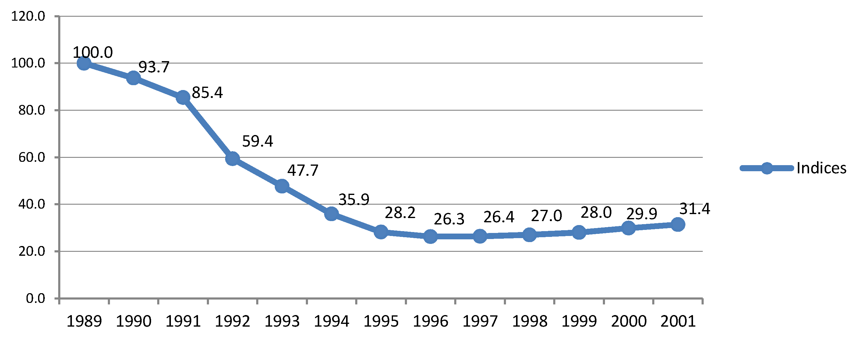
Figure 2.
Graphs of the logs (Panel: A) and growth rates (Panel: B) of the variables.

Table 1.
Sectoral Shares in Gross Domestic Product (percent).
| Years | Agriculture | Mining | Manufacturing | Utilities | Construction | Trade, Transportation. Accomodation., Food | Finance, Technical Services | Public Administration, Defence | Other Services |
|---|---|---|---|---|---|---|---|---|---|
| 2005 | 9.9 | 45.7 | 7.1 | 0.9 | 9.8 | 12.9 | 5.8 | 6.8 | 1.0 |
| 2006 | 7.5 | 53.3 | 6.0 | 0.8 | 8.2 | 11.2 | 5.8 | 6.6 | 0.6 |
| 2007 | 7.0 | 57.1 | 5.1 | 1.1 | 6.9 | 11.7 | 5.6 | 5.1 | 0.5 |
| 2008 | 6.0 | 56.0 | 5.0 | 1.3 | 7.4 | 12.0 | 5.8 | 5.9 | 0.7 |
| 2009 | 6.6 | 46.4 | 6.0 | 1.4 | 7.9 | 15.6 | 6.1 | 8.3 | 1.6 |
| 2010 | 5.9 | 49.2 | 5.0 | 1.1 | 8.7 | 14.0 | 6.6 | 7.5 | 1.8 |
| 2011 | 5.4 | 50.9 | 4.2 | 1.9 | 8.4 | 13.7 | 6.6 | 7.1 | 1.6 |
| 2012 | 5.5 | 45.9 | 4.5 | 2.2 | 10.7 | 14.1 | 7.7 | 7.5 | 1.8 |
| 2013 | 5.7 | 42.8 | 4.5 | 2.2 | 12.4 | 14.3 | 8.5 | 8.1 | 2.0 |
| 2014 | 5.7 | 37.0 | 5.1 | 2.1 | 13.6 | 15.7 | 9.7 | 8.6 | 2.3 |
| 2015 | 6.8 | 28.8 | 5.8 | 2.4 | 13.2 | 19.8 | 10.9 | 9.7 | 2.5 |
Source: Computed from National Accounts and Macroeconomic Indicators, Statistics Department to the State Statistical Committee of the Azerbaijan Republic, Table 2.4 labeled in Value Added by Industries at Current Prices (ISIC Rev 4) (http://www.stat.gov.az/source/system_nat_accounts/indexen.php).
Table 2.
Oil Revenues and Azerbaijan State Budget Relationship.
| Years | 2005 | 2006 | 2007 | 2008 | 2009 | 2010 | 2011 | 2012 | 2013 | 2014 | 2015 | 2016 |
|---|---|---|---|---|---|---|---|---|---|---|---|---|
| State Budget Revenues (million manat) | 2055 | 3881 | 6007 | 10,762 | 10,326 | 11,403 | 15,701 | 17,282 | 19,495 | 18,401 | 17,153 | 16,822 |
| Transfers from SOFAZ to the State Budget (million manat) | 150 | 585 | 585 | 3800 | 4915 | 5915 | 9000 | 9905 | 11350 | 9337 | 8130 | 7615 |
| Share of SOFAZ transfers in State Budget Revenues, percent | 7 | 15 | 10 | 35 | 48 | 52 | 57 | 57 | 58 | 51 | 47 | 42 |
| SOFAZ Revenues | 660 | 986 | 1886 | 11,864 | 8274 | 13,089 | 15,628 | 13,674 | 13,601 | 12,731 | 7721 | 8341 |
| Share of its transfers to the State Budget in SOFAZ revenues, percent | 23 | 59 | 31 | 32 | 59 | 45 | 58 | 72 | 83 | 73 | 105 | 91 |
| SOFAZ oil revenues from the oil PSAs (million manat) | 569 | 929 | 1800 | 11,633 | 7870 | 12,656 | 15,258 | 13,117 | 13,108 | 12,320 | 7370 | 8320 |
| Share of state budget transfers in the “Profit Oil”, percent | 26 | 63 | 33 | 33 | 62 | 47 | 59 | 76 | 87 | 76 | 110 | 92 |
Source: State Oil Fund of the Republic of Azerbaijan (SOFAZ) Annual Reports (2005–2013) and Central Bank of Azerbaijan (2014) Statistical Bulletin April 2014, and authors’ calculations (mainly about the ratios).
Table 3.
Azerbaijan: Consolidated Central Government Operations (2008–2015), in percent of non-oil GDP.
Table 3.
Azerbaijan: Consolidated Central Government Operations (2008–2015), in percent of non-oil GDP.
| Item | 2008 | 2009 | 2010 | 2011 | 2012 | 2013 | 2014 | 2015 Preliminary | 2016 Projection | 2017 Proj. | 2018 Proj. |
|---|---|---|---|---|---|---|---|---|---|---|---|
| Non-oil primary balance 1 | −39.2 | −35.5 | −36.3 | −40.3 | −45.4 | −45.6 | −35.8 | −34.4 | −37.7 | −32.6 | −31.8 |
| Share of public sector in fixed capital investments (percent of total) 2 | 54.4 | 42.8 | 38.6 | 42.7 | 43.8 | 48.7 | 42.3 | 41.9 | na | na | na |
1 This is defined as non-oil revenue minus expenditure (excluding interest payments) and statistical discrepancies. Sources: IMF (2013) Country Report No. 13/164, p. 27; IMF (2014) Country Report No. 14/159, p. 29; IMF (2016) Country Report No. 16/296, p. 4. 2 Sources: Central Bank of Azerbaijan (2008) Annual Report 2008, p. 17; Central Bank of Azerbaijan (2009) Annual Report 2009, p. 21; Central Bank of Azerbaijan (2011) Annual Report 2011, p. 13; Central Bank of Azerbaijan (2015) Annual Report 2015, pp. 15–16; National Bank of Azerbaijan (2007) Annual Report 2007, p. 19.
Table 4.
Descriptive Statistics of the Variables.
| Variable | Mean | Max | Min | Standard Deviation | Coefficient of Variation, % |
|---|---|---|---|---|---|
| Op | 0.608 | 1.109 | 0.216 | 0.268 | 44 |
| govcap | 364.596 | 1576.700 | 29.300 | 343.963 | 94 |
| noex | 216.391 | 496.438 | 87.821 | 83.948 | 39 |
| gdpno | 1951.575 | 4081.400 | 750.900 | 840.958 | 43 |
Table 5.
The Unit Root Test Results.
| Variable | Intercept | Intercept and Trend | ||||||
|---|---|---|---|---|---|---|---|---|
| Level | k | First Difference | k | Level | k | First Difference | k | |
| op | −0.950 | 2 | −6.411 *** | 1 | −3.495 * | 1 | −6.346 *** | 1 |
| govcap | −1.270 | 3 | −4.774 *** | 4 | −5.514 *** | 0 | −4.721 *** | 4 |
| noex | −1.840 | 3 | −7.442 *** | 2 | −2.374 | 3 | −7.365 *** | 2 |
| gdpno | −1.228 | 4 | −3.930 *** | 3 | −1.897 | 4 | −4.075 ** | 3 |
ADF denotes the Augmented Dickey-Fuller test. Maximum lag order is set to four and the optimal lag order (k) is selected based on the Schwarz criterion in the ADF test; ***, ** and * indicate rejection of the null hypotheses at the 1%, 5% and 10% significance levels, respectively; The critical values are taken from MacKinnon (1996) for the ADF test. The estimation period is 2000Q1–2013Q4.
Table 6.
Test Results for Optimal Lag Length Selection.
| Endogenous Variables: govcap and op | ||||||
|---|---|---|---|---|---|---|
| Lag | LogL | LR | FPE | AIC | SC | HQ |
| 0 | −188.066 | NA | 7.547 | 7.695 | 8.145 | 7.867 |
| 1 | 13.267 | 340.717 | 0.0038 | 0.105 | 0.705 | 0.335 |
| 2 | 28.490 | 24.591 | 0.0025 | −0.327 | 0.424 | −0.039 |
| 3 | 41.236 | 19.609 | 0.0018 * | −0.663 * | 0.238 * | −0.317 * |
| 4 | 42.170 | 1.365 | 0.0020 | −0.545 | 0.506 | −0.142 |
* indicates lag order selected by the criterion; LR is sequential modified LR (Likelihood Ratio) test statistic (each test at 5% level); FPE denotes Final prediction error, AIC, SC and HQ represent the Akaike, Schwarz and Hannan-Quinn information criteria, respectively.
Table 7.
Results of Cointegration Tests and Cointegration Equations.
| Panel A: Johansen’s Cointegration Test Results a | ||||
| Number of CE | Trace Statistics | Max-Eigenvalue Statistics | ||
| None | 23.843 *** | 23.812 *** | ||
| At most 1 | 0.0295 | 0.0295 | ||
| Panel B: Results of the Phillips-Ouliaris Cointegration Tests b | ||||
| Dependent Variable | z-Statistic | p-Values | tau-Statistic | p-Values |
| govcap | −32.153 | 0.000 *** | −5.004 | 0.000 *** |
| Panel C: Results of Cointegration Equations c | ||||
| Variable | VECM | FMOLS | DOLS | |
| op | 2.13 *** (0.000) | 1.99 *** (0.000) | 1.91 *** (0.000) | |
a The test type is Intercept and no trend in the cointegrating equation and the VAR; Critical values are taken from MacKinnon et al. (1999); CE means cointegrating equation(s); Estimation period: 2001Q1–2013Q4; b The null hypothesis for both tests is: variables are not cointegrated and is rejected; p-values are MacKinnon (1996) p-values for the tau-statistic; c The dependent variable is govcap. Estimation period is 2001Q1–2013Q4. p-values are in parentheses. The Speed of Adjustment Coefficient in the VECM equation is found to be (−0.45) and statistically significant at the 1% significance level. For all panels ***, ** and * indicate significance of the coefficients at the 1%, 5% and 10% significance levels, respectively.
Table 8.
Results of Cointegration Tests and Cointegration Equations.
| Panel A: Johansen’s Cointegration Test Results a | ||||
| Number of CE | Trace Statistics | Max-Eigenvalue Statistics | ||
| None | 23.042 *** | 19.395 *** | ||
| At most 1 | 3.646 | 3.646 | ||
| Panel B: Results of the Engle-Granger Cointegration tests b | ||||
| Dependent Variable | z-Statistic | p-Values | tau-Statistic | p-Values |
| noex | −24.731 | 0.000 *** | −3.448 | 0.000 * |
| Panel C: Results of Cointegration Equations c | ||||
| Variable | VECM | FMOLS | DOLS | |
| govcap | −0.233 *** (0.000) | −0.112 *** (0.000) | −0.121 *** (0.000) | |
a The null hypothesis for both tests is: variables are not cointegrated; ***, ** and * denote rejection of the null hypothesis at the 1, 5 and 10% significance levels, respectively; p-values are MacKinnon (1996) p-values for the tau-statistic; b The dependent variable is non-oil export. The estimation period is 2001Q1–2013Q4. p-values are in parentheses. ***, ** and * indicate significance of the coefficients at the 1%, 5% and 10% significance levels, respectively. Speed of Adjustment Coefficient in VECM equation is found to be (−0.43) and statistically significant at 1% significance level.
Table 9.
Results of Cointegration Tests and Cointegration Equations.
| Panel A: Johansen’s Cointegration Test Results a | ||||
| Number of CE | Trace Statistics | Max-Eigenvalue Statistics | ||
| None | 16.418 ** | 13.0986 * | ||
| At most 1 | 3.319 | 0.998 ** | ||
| Panel B: Results of the Phillips-Ouliaris Cointegration tests b | ||||
| Dependent Variable | z-Statistic | p-Values | tau-Statistic | p-Values |
| gdpno | −31.406 | 0.000 *** | −4.753 | 0.000 *** |
| Panel C: Results of Co-integration Equations c | ||||
| Variable | VECM | FMOLS | DOLS | |
| govcap | 0.452 *** (0.000) | 0.381 *** (0.000) | 0.388 ** (0.000) | |
a The test type is Intercept and no trend in co-integrating equation and the VAR; Critical values are taken from MacKinnon et al. (1999); CE means co-integrating equation(s); Estimation period: 2001Q1–2013Q4; b The null hypothesis for both tests is: variables are not cointegrated; p-values are MacKinnon (1996) p-values for the tau-statistic; c Dependent variable is non-oil GDP. Estimation period is 2001Q1–2013Q4. p-values are in parentheses. Speed of Adjustment Coefficient in VECM equation is found to be (−0.02) and statistically insignificant. For all panels ***, ** and * indicate significance of the coefficients at the 1%, 5% and 10% significance levels, respectively.
© 2017 by the authors. Licensee MDPI, Basel, Switzerland. This article is an open access article distributed under the terms and conditions of the Creative Commons Attribution (CC BY) license (http://creativecommons.org/licenses/by/4.0/).
Share and Cite
MDPI and ACS Style
Gurbanov, S.; Nugent, J.B.; Mikayilov, J. Management of Oil Revenues: Has That of Azerbaijan Been Prudent? Economies 2017, 5, 19. https://doi.org/10.3390/economies5020019
AMA Style
Gurbanov S, Nugent JB, Mikayilov J. Management of Oil Revenues: Has That of Azerbaijan Been Prudent? Economies. 2017; 5(2):19. https://doi.org/10.3390/economies5020019
Chicago/Turabian StyleGurbanov, Sarvar, Jeffrey B. Nugent, and Jeyhun Mikayilov. 2017. "Management of Oil Revenues: Has That of Azerbaijan Been Prudent?" Economies 5, no. 2: 19. https://doi.org/10.3390/economies5020019
Note that from the first issue of 2016, this journal uses article numbers instead of page numbers. See further details here.