
The Nonlinearity of the New Keynesian Phillips Curve: The Case of Tunisia

Department of Economics, Faculty of economics and Management, University of Sfax, 3026 Sfax, Tunisia
*
Author to whom correspondence should be addressed.
Economies 2017, 5(3), 24; https://doi.org/10.3390/economies5030024
Submission received: 27 December 2016
/
Revised: 30 May 2017
/
Accepted: 20 June 2017
/
Published: 7 July 2017
Abstract
:This article seeks to check the nonlinearity of the Phillips curve in Tunisia for the 1993–2012 period, relying on a hybrid new Keynesian Phillips curve modeled via a Logistic Smooth Transition Regression (LSTR) model with endogenous variables. We estimate this model using the nonlinear instrumental variables. The empirical results corroborate the new Keynesian assumption ofprice rigidity and show that the response of inflation to the output gap tends to be significant only if the inflation rate tends to be relatively high and exceeds a certain threshold. For a low inflation rate, the price rigidity dominates. This result is particularly evident in Tunisia, especially for the years following the 2011 revolution during which the elasticity of inflation rate to an excess demand has become highly important and the inflation rate experienced record levels.
JEL Classification:
C22; C52; E31; E581. Introduction
Specifying the nature of the aggregate supply curve is of crucial importance for the conduct of monetary policy to the extent that it determines the mechanisms that convey the actions taken by the central bank to the economy. The central bank, in manipulating the policy instrument, acts according to the ability of production to influence the price level and to the intensity of this influence. Therefore, an appropriate monetary policy depends to a large extent on the nature of the inflation-production specification. This relationship has been apprehended under the famous Phillips curve originally proposed by Phillips in 1958.
The short term Phillips curve is commonly analyzed in a linear framework implying a stable relationship between inflation and economic activity which does not depend on the macroeconomic conditions. The variation in the actual production compared to its potential is associated with a simple proportional change in inflation in the same direction. However, the increased complexity of the relationship between the real and financial sphere and the nominal wage and price rigidity that characterizes the nineties favored the emergence of a new strand of both theoretical and empirical literature that claims to the asymmetry of the inflation-output relationship. This asymmetry implies that short-term effect of the output gap on inflation depends either on the initial inflation level (low or high inflation) or on the state in the business cycle (expansion or recession) resulting in a non-linear Phillips curve.
Recent studies tend to give support to this non-linear hypothesis. Villavicencio and Mignon (2013) show that the output-inflation relationship depends on the trend of inflation for six developed countries. The sensitivity of inflation to the output gap is increasing from a certain level of inflation that erodes price rigidity. Ball and Mazumder (2011) evidence that the Phillips curve in the United States has been relatively flat in the low-inflation period since the mid-1980s. In their estimation, the Phillips curve has flattened post-1984, and the 1985–2007. Hasanov et al. (2010) claim that inflation-production trade off in Turkey changes rapidly from low-inflation regime to high inflation regime leading to a convex Phillips curve during 1998–2008. With time-varying persistence models, Mladenovic and Nojkovic (2012) show that inflation persistence randomly changes between two regimes in many countries of Central and Southeastern Europe. Eliasson (2001) finds evidence in favor of the non-linearity of the Phillips curve in Sweden. The rate of change of inflation depends strongly on inflation expectations. However, some other studies show that the asymmetry of the Phillips curve depends on the state of the economy. Thus, the response of inflation to the output gap could be higher during a period of expansion than during a recession (convex Phillips curve). Periods of euphoria may be more inflationary than recessions are deflationary (Clark et al. 1996; Debelle and Laxton 1997; Huh and Jang 2007; Dolado et al. 2005; Debelle and Vickery 1998; Alvarez 2000). On the contrary, Eisner (1997), Turner (1997) and Nell (2006) conclude in favor of the concavity of the Phillips curve implying that the effect of a change in the output gap on inflation is more important in recessionary periods.
Over the past decade, the achievement of the price stability objective became the primary concern of monetary policy in Tunisia. To carry out its mission, the Central bank of Tunisia (BCT) had to establish a system of inflation analysis and estimates in the short and middle terms, serving as a reference for the decision-making process in monetary policy. In fact, since 2007, the Central Bank of Tunisia (BCT) has implemented an ambitious strategy to manage inflation and serious attempts are being implemented in order to establish a device for analyzing and forecasting inflation relying on a wide range of indicators closely linked to inflation such as import prices, the output gap, core inflation, etc. Understanding the nature of the relationship between inflation and output is of great importance to the Tunisian monetary authorities since it can guide their behavior and the intensity of their reactions. Empirically, several authors have examined the inflation–output relationship in the case of Tunisia. Agénor and Bayraktar (2008) used a hybrid new Keynesian Phillips curve to describe the dynamics of inflation in Tunisia. They find that the retrospective behavior of firms seems more dominant and the output gap does not have a significant impact on the inflation process in Tunisia. Dammak and Boujelbène (2009) introduced a downward nominal wage rigidity variable in the Phillips curve model. Although this variable is significant, it does not have a sign consistent with the theory, but the Phillips curve remains valid. In the long term, it is not vertical.
Our approach in this paper is different from previous research on Tunisia. This article aims to have a better understanding of the nature of the inflation-output trade-off in Tunisia by testing the existence of a possible non-linearity in this relationship. Given the lack of theoretical consensus on a particular form of non-linear Phillips curve, we used a modeling strategy to estimate a nonlinear model without resorting to preliminary assumptions about the functional form that this curve may take. This is a more general approach characterized by greater flexibility, providing an approximation for the generation process of different data: the smooth transition regression model (STR), see Granger and Teräsvirta (1993), Teräsvirta (1998, 2006).
The remainder of this paper is organized as follows: Section 2 presents a theoretical framework of the linear and nonlinear Phillips curve. Section 3 introduces a description of the econometric model and the data. Section 4 illustrates the estimations and empirical results and Section 5 provides concluding remarks.
2. Literature Review
2.1. Linear Phillips Curve Modeling
The nominal rigidity that characterizes the eighties and nineties combined with the hypothesis of rational expectations have fostered the emergence of the “new Keynesian Phillips curve” based on microeconomic foundations of optimal behavior of economic agents. The main assumption of the New Keynesian approach is based on the earlier study of Calvo (1983) using staggered nominal wage contracts and price setting by forward looking individuals and firms. Firms maximize the expected value of future profits being constrained by the costs of price adjustment. The presence of these costs may lead them to choose to keep a fixed price for several periods. So, there are a fraction of firms “α” that adjust their prices and a fraction (1 − α) which maintains their prices fixed. The linear new Keynesian Phillips curve is typically assumed to have the following form:
The main criticism of the New Keynesian Phillips curve relates to its purely forward-looking features, it does not imply persistence of inflation (Rudd and Whelan 2005). To this end, a so-called “hybrid version” of the new Keynesian curve was proposed to introduce some inertia in inflation dynamic. Gali and Gertler (1999) assume that among the firms that redefine their prices, a fixed proportion “w” uses a backward-looking price setting rule. This hybrid curve is therefore a combination of backward and forward-looking components. Thus,
This can be viewed as a mixture between the traditional and the “new” Phillips curve. Recent studies, in particular by Rudd and Whelan (2007), cast doubt on the ability of the NKPC (including its hybrid form) to provide a useful empirical characterisation of the inflation process. Gordon (2011) formulate a new specification baptized “new Keynesian Triangle Phillips curve” that features an expectational element, excess demand pressure (output-gap) and “supply shock” variables and find that this formulation outperforms the NKPC.
2.2. Micro Foundations for a Non-Linear Phillips Curve
According to the models presented in the previous section, the tradeoff between inflation and production is assumed to be constant. However, various theoretical models argue that the slope of the Phillips curve depends on the state of the economy or on the level of inflation.
In the monopolistic competitive model Stiglitz (1984), for example, firms are the source of any policy pricing. They may choose to decrease their prices in order to keep their market share, but they are reluctant to raise them in order to prevent the arrival of new competitors (even if the general price level is high). Hence, they may respond to an increase in economic activity with more muted price changes and larger output changes than to a similar decrease in economic activity. The reduced sensitivity of inflation as the economy strengthens implies that the shape of the Phillips curve is concave. In the capacity constraint model, on the other hand, inflation will be increasingly sensitive to changes in output as the economy strengthens. Economic expansion is limited by capacity constraints. These constraints can be the result of a technical failure or lack of labor, which makes firms unable to increase production in the short term to keep with an increase in demand. They then opt to increase their prices. Therefore, inflation widens with increasing frequency as output continues to rise. Inflation is more sensitive to output during periods of excess demand than in a situation of excess supply. The Phillips curve, then takes a convex shape (Alvarez 2000). There are also models suggesting that the relationship between output and inflation may vary with the level of inflation. In the downward nominal wage rigidity model, for example, workers are victims of a money illusion. They are more reluctant to accept a reduction in their nominal wages than a drop in their real wages generated by higher inflation. In low-inflation regime, the downward rigidity of nominal wages is an obstacle against the real wage adjustment. Therefore, excess supply has eventually less impact on prices than excess demand giving rise to a convex relation between inflation and the output gap. Analogously, in the menu cost model, for example, if inflation tends to increase, the current price of the firm goes largely away from the desired price level. Faced with a given shock, the profit on changing price is more important than the cost incurred. So, firms can be encouraged to adjust their prices (Ball and Mankiw 1994). Firms will increase the frequency and the size of price adjustment as inflation rises, so that aggregate demand shocks will have more effect on the price level, but less effect on output (Ball et al. 1988). Finally, the signal extraction model (Lucas 1973) assumes that firms are unable to distinguish between changes in the aggregate price level and relative price movements since the shocks are unobservable. The relationship between output and inflation depends on the volatility of inflation. Thus, the more volatile the aggregate price index, the less changes in different prices are attributed to changes in relative prices and consequently the level of production does not record any change. The resulting short-run Phillips curve has a positive slope that depends on the inflation volatility.
3. Methodology and Data
3.1. The Model
Different methodologies have been exploited by empirical studies on the nature of the short-term relationship between inflation and output. Some authors seek to determine if nominal demand shocks have asymmetric effects on real activity, while others are trying to identify a non-linear Phillips curve in a specific functional form. In this study, we use the smooth transition regression model (STR) proposed by Granger and Teräsvirta (1993), Teräsvirta (1998, 2006). Smooth transition regression (STR) models have several advantages over competing structural break and nonlinear models. First, this model allows the application of linearity tests and modeling the process of regime switching without requiring a prior non-linear functional form. Second, STR models are theoretically more appealing over simple threshold and Markov regime switching models, which impose an abrupt change in the coefficients. Instantaneous changes in regimes are possible only if all agents act simultaneously and in the same direction. For the market of many traders acting at slightly different times, a smooth transition model is more appropriate (Hasanov et al. 2010). Third, this model can provide a good framework to study possible non linearity in the interrelationship between the inflation rate and output since it allows an economic intuition for the nonlinear dynamic identifying why and when inflation sensitivity changes toward output fluctuations.
The STR model has the following form:
where is the vector of explanatory variables, are parameters to be estimated in the linear and nonlinear part respectively. The error term is assumed to be independent and identically distributed with zero mean and constant variance . The transition function is a continuous function of the transition variable () and ranges from 0 to 1. is a location parameter of the threshold that indicates where the change occurs and the slope parameter “” measures the smoothness of the transition from one regime to another. The transition function can be either exponential or logistics. This paper considers a logistic function (LSTR) as follows:
This transition function G(.) varies with the extent of the difference between the transition variable in relation to the threshold (c). If this difference is negative () then the transition function is equal to 0 and inflation-production tradeoff is summarized by the coefficients of the linear part. However, when the difference is positive ( > c), the transition function tends to 1 and the parameters describing this relationship are equal to the combination of the linear and nonlinear coefficients (). The slope of the Phillips curve will be specified by a continuum of parameters between the two regimes.
In general, the specification of the appropriate LSTR model to describe the nonlinear dynamics of inflation must go through three key stages. The first is to determine an appropriate linear model that serves as a basis for the test of linearity against LSTR model. Then, a linearity test must be applied in order to validate the existence of non-linearity in the response of inflation and determine the transition variable according to which the inflation changes its reaction to the output gap. Once linearity is rejected, we proceed to the estimation of the nonlinear model specified.
Testing linearity against the alternative of an LSTR (k) model amounts to testing if = 0 in Equation (4). The model is not identified under the null hypothesis due to the nuisance parameters and c. A Taylor series approximation about = 0 is used as a substitute to circumvent this problem, and the tests are based on this transformed equation (see Teräsvirta 1998 and Van Dijk et al. 2002):
with = , with the remainder and where is (h×1) vector of explanatory variables and is the transition variable. The null hypothesis imply H01: = 0 against the alternative H11 at least , j = 1, 2, 3. It can be checked by means of an LM test with asymptotic chi-squared distribution, but in small sample it is recommended to rely on the Fisher statistic because it has good size properties. This test can be applied to one or more variables in the model. If linearity is rejected for more than one variable, the transition variable selected will be that associated with the lowest p-value for the rejection of linearity. In order to decide between k = 1 and k = 2, one continues by carrying out the following test sequence within Equation (5):
According to Granger and Teräsvirta (1993), if the p-value for the rejection of H03 is the smallest an LSTR (2) model is chosen otherwise, an LSTR (1) model is selected.
3.2. Data Description
In this paper, we consider quarterly data collected for Tunisia from the International Monetary Fund’s IFS database (CD-ROM). They cover the period from 1993:1 to 2012:3. Inflation has been calculated as the annual rate of change of the consumer price index. Regarding the potential output, it is calculated using the Hodrick-Prescott filter, and the output gap corresponds to the difference, in percentage points, between the industrial production index and its potential value.
The specification procedures described in the previous section rely on the assumption that both the output gap and inflation rate are I(0) processes. Therefore, prior to the estimation of the linear model, we tested stationarity of the variables concerned with the conventional ADF and KPSS unit-root tests. The results of these tests are provided below in Table 1.
4. Estimation and Empirical Results
4.1. Specification and Estimation of the Linear Phillips Curves
In what follows, we will try to estimate the two versions of the new Keynesian Phillips curve proposed in the literature (forward looking and hybrid) in order to determine whether the dynamics of inflation in Tunisia can be explained by a linear inflation-output relationship. The estimation of these two versions of the Phillips curve will allow us to select which to base the linearity test.
Both forms of the hybrid and forward looking Phillips curve are based on the central hypothesis of rational expectations. Such expectations imply an orthogonality condition for measuring the informational efficiency of the expectations. This rationality assumes that the forecast errors are orthogonal to all information available.
Gali and Gertler (1999) estimate these forms of the Phillips curve by GMM making use of lagged instrumental variables. They consider four lags for inflation, the labor share of income, output gap, the difference in rates (long 10-month rate, short 3-month rate), wage inflation and inflation commodity. In contrast, Gali et al. (2005) choose a smaller number of instruments in order to minimize the estimation bias due to the number of over-identifying restrictions.
According to the literature, we estimate our models (Equations(1) and (2)) through the generalized method of moments replacing future expected inflation rate by future realized inflation rate in Equations (1) and (2). One implication of rational expectations is that valid instruments may be weak instruments. As a practical solution, we include the lag of independent variables. So, the instruments used consist of four lags of inflation, output gap and short-term interest rate. The validity of these instruments was verified by Hansen (1982) J-test for overidentification, which is used to test the orthogonality of the instruments to the perturbation term.
The GMM estimates of the two inflation equations are given below in Table 2.
The forward Phillips curve shows that the prospective component of inflation seems to contribute to the development of inflation in Tunisia since the coefficient inherent in the anticipated future inflation is significant and positive, but the output gap has no influence on inflation, its coefficient is insignificant. The estimate of the hybrid Phillips curve highlights the importance of the previous level of inflation which implies that part of the Tunisian companies use retrospective mechanisms to adjust their prices. The prospective component maintains its significance attributing some importance to the expectations of future inflation. The coefficient of the output gap appears statistically different from zero, but it has a negative sign. This negative sign of the output gap coefficient calls into question the relevance of this inflation-output relation.
We can conclude that the linear Phillips curve is not able to provide a perfect description of the process of inflation in Tunisia. The linear specification may be too restrictive because it does not account for potential nonlinear effects coming from the macroeconomic environment. In other words, the effect of excess demand on inflation is assumed to be the same independently of the state of the economy or the initial level of inflation.
So, we challenge the assumption of linear Phillips curve and test for the non-linearity of this relationship based on the hybrid model since forward-looking behavior is as important as backward-looking behavior in determining inflation in Tunisia.
Since the nonlinearity tests are sensitive to residual properties and in particular to autocorrelation, we conducted diagnostic tests for the hybrid model residuals. Table 3 shows neither conditional heteroscedasticity nor autocorrelation. Furthermore, residuals do not suffer from excess kurtosis and skewness, and are normally distributed.
4.2. Linearity Tests and LSTR Estimation
As the model seems to be satisfactory, now we proceed to test linearity on the basis of the selected hybrid curve to check the existence of a non-linear relationship and determine the transition variable which controls the regime change. The applied test assumes the null hypothesis of linearity against LSTR alternative as suggested by Teräsvirta (1998). It is performed for various explanatory variables included in the hybrid model, i.e., past inflation, future inflation and the output gap. The results of the linearity tests are provided in Table 4. The table also reports specification tests of Granger and Teräsvirta (1993) to choose the appropriate transition function that governs regime change.
As can readily be seen from Table 4, the null hypothesis of linearity is rejected for lagged inflation only. This finding implies that inflation behavior exhibits a switching regime governed by the level of inflation realized in the previous period. The used transition variable is past inflation suggesting that the relationship between inflation rate and the output gap depends upon the inflation trend (low or high inflation level).
The tests applied to choose a suitable transition function show that H02 is rejected more strongly, so we select a logistic transition function with a single threshold estimate. We can therefore begin estimating the following nonlinear smooth transition model (LSTR 1) which seems to be the more appropriate model for our data:
In this model, the two regimes are associated with small and large values of inflation. This type of regime-switching can be convenient for modeling asymmetric responses from a monopolistic price setter, where the regimes of the STR are related to the inflation environment. The parameter “c” can be interpreted as the inflation level that the price setter considers critical.
The estimation results of the LSTR model are provided in Table 5.
The results from the LSTR estimation clearly show that the relationship between output and inflation depends strongly on the inflation environment, justifying the use of our regime-switching model. Indeed, the threshold at which the change occurs is statistically different from zero and equal to 3.55%. Thus, when past inflation is less than 3.55% (at lower trend inflation), economic slack has no noticeable effect on inflation since the output gap coefficient is not significant (prices are rigid). However, for past inflation that exceeds the threshold (at higher trend inflation), the slope becomes positive and significant. The inflation sensitivity to output fluctuations becomes important as the rate of inflation increases and rises above the threshold level. These results are consistent with the costly price adjustment model (menu cost model) which recommends that in an environment of nominal price rigidity, a demand shock affects more intensively the price level during periods of high inflation since firms, operating under monopolistic competition, are encouraged to increase the frequency and intensity of their price adjustment. Excess demand will therefore have a significant impact on inflation when this latter is high.
Our results corroborate the nonlinearity of the inflation-output relationship in Tunisia depending on past inflation rate and provide the threshold that erodes price rigidity and tends to restore the inflation-output trade-off.
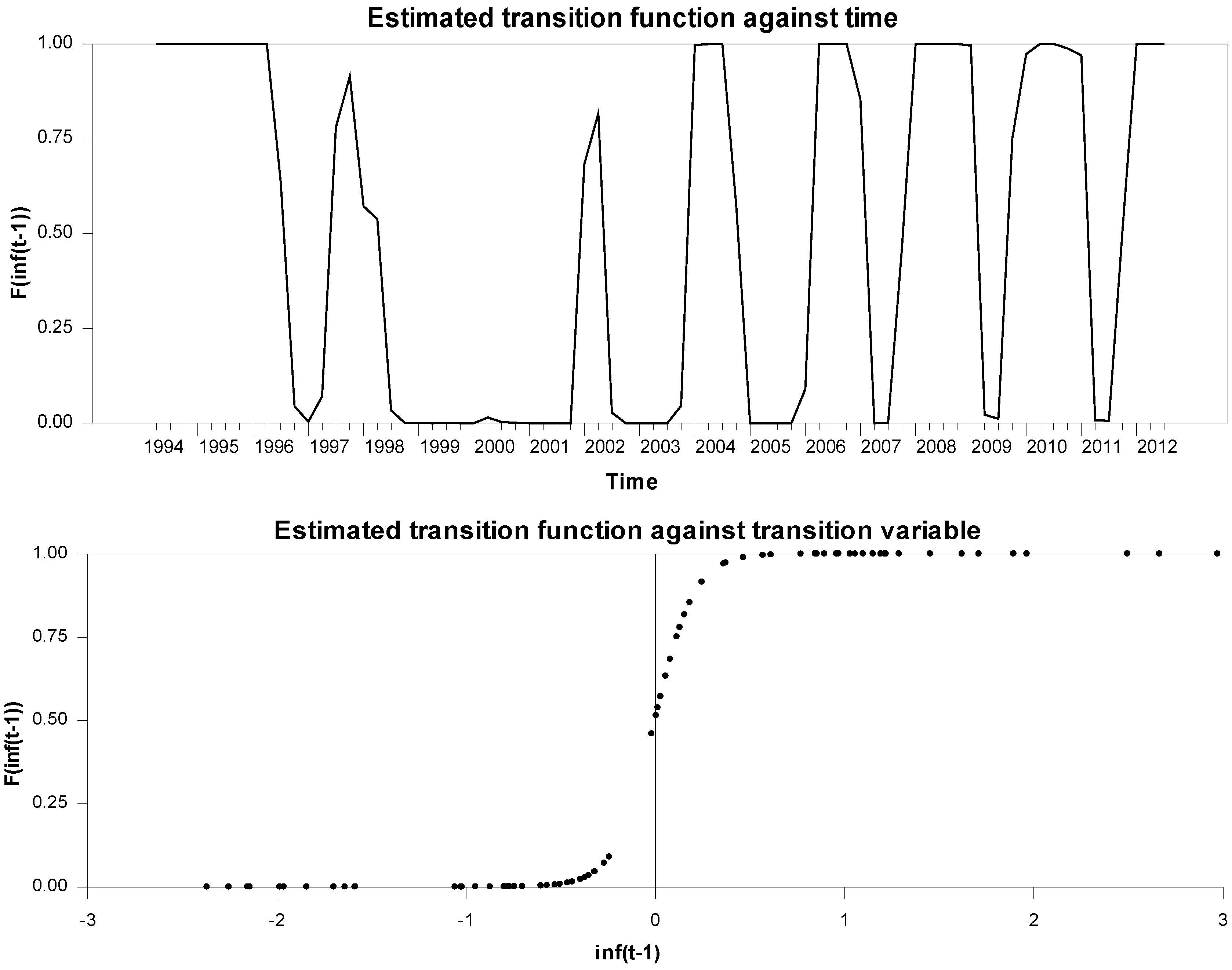
Figure 1 plots the graph 1 of the estimated transition function against transition variable as well as the graph 2 of the estimated transition function against time.
Graph 1 implies that the change in parameters of the estimated model happened gradually over time. This finding is very impressive, especially when the developments in the Tunisian economy during the last two decades are taken into account.
During the nineties, the sensitivity of inflation to economic activity was almost non-existent in Tunisia given the ambitious strategy of price administration followed by the government to control the general price level: in 1992, only 22% of product prices are not administered (Boughrara et al. 2010). Controlling inflation may reduce some of the pressure on the Tunisian dinar and ensure a greater stability of its value. A rule of constant real effective exchange rate was also considered in Tunisia to avoid a high depreciation or appreciation of the exchange rate which may lead to imported inflation or threaten the competitiveness of Tunisian firms.
From the start of the last decade, Tunisia has undertaken new reforms to lift price controls and achieve a gradual real and financial liberalization in order to converge to a functioning market economy. The strategy was that liberalization of imports and increased competition will help contain the inflation rate. The new policy of economic development relying on export promotion and trade liberalization required increased competitiveness of domestically produced products and the progressive dismantling of price controls. Besides, import regime was gradually liberalized, and foreign direct investments and export encouraging policies were followed. In addition, interest rates and exchange regime were gradually liberalized, and new market institutions were established step-by-step.
The estimated transition function in graph 1 indicates that these reforms in the Tunisian economy have led to significant changes in the inflation-output relationship since the end of 2003. Prices, being more flexible, can reflect more accurately the market conditions (supply and demand) and would depend on the reality of the macroeconomic environment in general. So, an excess demand can affect inflation rate and be associated with an increase in the price level.
Graph 2 indicates a smooth transition from two limiting regimes associated with the extreme values of the transition function (f{inf (t− 1)}) 0 and 1. The first regime is the “price-rigidity” regime when past inflation is below the threshold level. Whereas, the second regime reestablishes the inflation-output relationship if past inflation exceeds the threshold. At the estimated threshold between the two regimes which is equal to 3.55, the logistic transition function is equal to 0.5 and changes monotonically from 0 to 1 as past inflation tends to be more important and reaches the estimated threshold.
This result is particularly evident in Tunisia and especially in the last years following the 2011 revolution during which the elasticity of inflation rate to an excess demand has become highly important and inflation rate has experienced record levels. In fact, when the inflation rate reached the threshold level and passed to 4.2% in 2011 (annual rate of change), excess demand arising from Libya for fresh food and Agri-food manufactured products, has led to a significant rise in inflation reaching 5.9% in 2012. Indeed, due to the high inflation environment, firm’s current prices are outside the optimum level and firms find it convenient, after the demand shock, to increase their prices despite the menu cost that would be supported.
Our results have important policy implications. In fact, as there is no relationship between inflation and output, the Phillips curve remains flat until inflation reaches a certain threshold, so inflation control becomes an easy task when the price level is low, since adjustments to excess demand are not instantaneous and slow. Thus, when inflation is below the estimated thresholds, monetary authorities could reduce the interest rate to stimulate economic activity without fear of inflationary pressures. Nevertheless, exceeding the threshold may introduce significant inflationary pressures in the economy and monetary authorities are required to increase more vigorously their instrument in order to contain these inflationary pressures mainly after the revolution.
Tunisian monetary authorities must take into account the nonlinearity detected in the inflation-output relationship and adopt a nonlinear reaction function to avoid inflationary bias. However, Kobbi and Gabsi (2014) shows that the nonlinearity detected in the BCT’s reaction is inconsistent with the behavior of a central bank aimed at price stability. It adjusts the interest rate down more importantly, when inflation is low than the upward adjustment of the rate in the case of high inflation rate. This asymmetry is due to the multiplicity of the monetary policy objectives assigned to the BCT, which are sometimes contradictory (financial stability, economic growth and price stability), as well as the absence of a real liberalization of interest rates. The BCT’s reluctance to significantly increase the interest rate when the level of inflation is high stem from its concern to sustain economic growth and to ensure financial stability of a banking system highly fragile due to its low level of capitalization and the existence of a high level of non-performing loans specially after the 2011 revolution. All this can prevent the BCT to properly fulfill its mission of preserving price stability through interest rate policy which explains the high level of inflation favored by a nonlinear economic structure.
5. Conclusions
In this paper, we investigate possible nonlinearity in the inflation-output relationship in Tunisia. For this purpose, we first estimate a linear hybrid new Keynesian Phillips curve for the 1993–2012 period using quarterly data and then test for the non-linear alternative. The test results suggest that the sensitivity of inflation to output depends on the initial rate of inflation. To estimate the non-linear specification, we rely on the logistic smooth transition regression (LSTR) model employing the non-linear instrumental variables method to take into account the endogeneity problem. Our results show the predominance of two regimes. The first is a price rigidity regime associated with a low inflation rate in which output has no effect on inflation rate, whereas the second restores the inflation output tradeoff since inflation become more important. Thus, there is an estimated threshold of inflation, equal to 3.55% that erodes price rigidity and increases the inflation sensitivity to an excess demand.
Not taking into account the non-linearity inherent in the Phillips curve is probably associated with an inefficient monetary policy. Thus, actions based on the assumption that the Phillips curve is a linear result of systematic errors in fulfilling the objective of price stability and inflation tend to be on average higher than its target. Therefore, Tunisian monetary authorities must take account of this asymmetry in the conduct of monetary policy by trying to adjust their instrument in a more important way during periods of high inflation to counteract inflationary pressures resulting from exogenous demand shocks.
Author Contributions
Kobbi Imen was responsible for conceptualizing the paper, framing its research objectives, identifying a suitable empirical methodology and ensuring overall quality control of the paper; while Foued Gabsi contributed mainly into the interpretation of empirical results of the paper.
Conflicts of Interest
The authors declare no conflict of interest.
References
- Agénor, Pierre-Richard, and Nihal Bayraktar. 2008. Contracting Models of the Phillips Curve Empirical Estimates for Middle-Income Countries. Discussion Paper Series, n° 094; Manchester: University of Manchester. [Google Scholar]
- Alvarez, Lois P. 2000. Endogenous Capacity Utilization and the Asymmetric Effects of Monetary Policy; WP 469. UFAE (Unitat de Fonaments de l’Anlisi Econmica) and IAE (Institut d’Anlisi Econmica). Available online: http://www.recercat.cat/bitstream/handle/2072/1978/46900.pdf?sequence=1 (accessed on 3 July 2017).
- Ball, Laurence, and Gregory N. Mankiw. 1994. Asymmetric Price Adjustment and Economic Fluctuations. Economic Journal 104: 247–61. [Google Scholar] [CrossRef]
- Ball, Laurence M., and Sandeep Mazumder. 2011. Inflation Dynamics and The Great Recession, Brookings Papers on Economic Activity. Washington: The Brookings Institution, vol. 42, pp. 337–405. [Google Scholar]
- Ball, Laurence, Gregory N. Mankiw, and David Romer. 1988. The New Keynesian Economics and the Output-Inflation Trade-off. Brookings Papers on Economic Activity 1: 1–65. [Google Scholar] [CrossRef]
- Boughrara, Adel, Mongi Boughzala, and Hassouna Moussa. 2010. Financial Fetters of the Monetary Policy of Tunisia to be presented in the Vlème Colloque International. Hammamet: Prospectives Stratégies E Développent Durable. [Google Scholar]
- Calvo, Guillermo A. 1983. Staggered Prices in a Utility Maximising Framework. Journal of Monetary Economics 12: 383–98. [Google Scholar] [CrossRef]
- Clark, Peter B., Douglas Laxton, and David Rose. 1996. Asymmetry in the U.S. Output-Inflation Nexus: Issues and Evidence. IMF Staff Papers 43: 216–51. [Google Scholar] [CrossRef]
- Dammak, Thouraya, and Younès Boujelbène. 2009. The long run Phillips curve and the role of downward nominal wage rigidity in Tunisia. Economics Bulletin 29: 1211–23. [Google Scholar]
- Debelle, Guy, and Douglas Laxton. 1997. Is the Phillips Curve Really a Curve? Some Evidence for Canada, the United Kingdom, and the United States. IMF Staff Papers 44: 249–82. [Google Scholar] [CrossRef]
- Debelle, Guy, and James Vickery. 1998. Is the Phillips Curve a Curve? Some Evidence and Implications for Australia. Economic Record 74: 384–98. [Google Scholar] [CrossRef]
- Dolado, Juan J., Pedrero Ramón Maria-Dolores, and Manuel Naveira. 2005. Are Monetary Policy Reaction Functions Asymmetric? The Role of Non-linearity in the Phillips Curve. European Economic Review 49: 485–503. [Google Scholar] [CrossRef]
- Eisner, Robert. 1997. A New View of the NAIRU. In Improving the Global Economy. Edited by Paul Davidson and Jan A. Kregel. Cheltenham: Edward Elgar, pp. 196–230. [Google Scholar]
- Eliasson, Ann-Charlott. 2001. Is the Short-run Phillips Curve Nonlinear? Empirical Evidence for Australia, Sweden and the United States. Working Paper Series n° 124; Stockholm: SverigesRiksbank. [Google Scholar]
- Gali, Jordi, and Mark Gertler. 1999. Inflation Dynamics: A Structural Econometric Analysis. Journal of Monetary Economics 44: 195–222. [Google Scholar] [CrossRef]
- Gali, Jordi, Mark Gertler, and David Lopez-Salido. 2005. Robustness of the Estimates of the Hybrid New Keynesian Phillips Curve. Journal of Monetary Economics 52: 1107–18. [Google Scholar] [CrossRef]
- Gordon, Robert. 2011. The history of the Phillips curve: Consensus and bifurcation. Economica 78: 10–50. [Google Scholar] [CrossRef]
- Granger, Clive, and Timo Teräsvirta. 1993. Modelling Nonlinear Economic Relationships. New York: Oxford University Press. [Google Scholar]
- Hansen, Lars P. 1982. Large Sample Properties of Generalized Method of moments Estimators. Econometrica 50: 1029–54. [Google Scholar] [CrossRef]
- Hasanov, Mübariz, Aysen Araç, and Funda Telatar. 2010. Nonlinearity and Structural Stability in the Phillips curve: Evidence from Turkey. Economic Modelling 27: 1103–15. [Google Scholar] [CrossRef]
- Huh, Hyeon-seung, and Inwon Jang. 2007. Nonlinear Phillips curve, Sacrifice ratio, and the Natural rate of Unemployment. Economic Modelling 24: 797–813. [Google Scholar] [CrossRef]
- Kobbi, Imen, and Foued Gabsi. 2014. L’asymétrie de la politique monétaire en Tunisie: Estimation d’unerègle forward-looking non linéaire pour la Banque centrale. Economie Appliquée 67: 139–68. [Google Scholar]
- Lucas, Robert. 1973. Some International Evidence on Output-Inflation Tradeoffs. American Economic Review 63: 326–34. [Google Scholar]
- Mladenovic, Zorica, and Aleksandra Nojkovic. 2012. Inflation Persistence in Central and Southeastern Europe: Evidence from Univariate and Structural Time Series Approaches. Panoeconomicus 2: 255–66. [Google Scholar] [CrossRef]
- Nell, Kevin. 2006. Structural Change and Nonlinearities in a Phillips Curve Model for South Africa. Contemporary Economic Policy 24: 600–17. [Google Scholar] [CrossRef]
- Rudd, Jeremy, and Karl Whelan. 2005. New tests of the new-Keynesian Phillips curve. Journal of Monetary Economics 52: 1167–81. [Google Scholar] [CrossRef]
- Rudd, Jeremy, and Karl Whelan. 2007. Modelling inflation dynamics: A Critical Review of Recent Research. Journal of Money, Credit, and Banking 39: 155–70. [Google Scholar] [CrossRef]
- Stiglitz, Joseph E. 1984. Price Rigidities and Market Structure. American Economic Review 74: 350–55. [Google Scholar]
- Teräsvirta, Timo. 1998. Modeling Economic Relationships with Smooth Transition Regressions. Handbook of Applied Economic Statistics. Edited by Ullah Aman and David Giles. New York: Dekker, chapter 15. pp. 507–52. [Google Scholar]
- Teräsvirta, Timo. 2006. Chapter 8 Forcasting Economic Variables with Nonlinear Models. In Handbook of Economic Forecasting. Edited by Graham Elliott, Clive W.J. Granger and Allan Timmermann. Amsterdam: Elsevier, vol. 1, pp. 413–57. [Google Scholar]
- Turner, Paul. 1997. The Phillips Curve, Parameter Instability and the Lucas Critique. Applied Economics 29: 7–10. [Google Scholar] [CrossRef]
- Villavicencio, Antonia, and Valérie Mignon. 2013. Nonlinearity of the Inflation-Output Trade-Off andTime-Varying Price Rigidity. WP No. 2. Paris: CEPII. [Google Scholar]
- Van Dijk, Dick, Timo Teräsvirta, and Philip Franses. 2002. Smooth Transition Autoregressive Models: A Survey of Recent Developments. Econometric Reviews 21: 1–47. [Google Scholar] [CrossRef]
Figure 1.
Estimated transition function.

Table 1.
Unit-root tests results.
| Variable | ADF Test | KPSS Test |
|---|---|---|
| Inflation | −5.158*** | 0.262*** |
| Output gap | −4.397*** | 0.139*** |
Notes: Test regressions include only an intercept term *, **, *** denote rejection of the null hypothesis of a unit root at 10%, 5% and 1% significance level, respectively.
Table 2.
Linear Phillips curves estimations.
| AIC | SBC | J-STAT | ||||
|---|---|---|---|---|---|---|
| Forward | - | 1.078 ** | 0.037 | 259.681 | 266.426 | 12.69 |
| (0.045) | (0.038) | (0.241) | ||||
| Hybrid | 0.505 ** | 0.601 ** | −0.053 ** | 182.155 | 191.149 | 11.69 |
| (0.035) | (0.041) | (0.018) | (0.23) |
Notes: Standard errors are given in parentheses; significance level at which the null hypothesis is rejected: **, 5%; and *, 10%. AIC denotes Akaike Information Criterion, SBC denotes Schwarz Information criteria and J-STAT denotes Hansen (1982) overidentification test. Heteroscedasticity and autocorrelation consistent standard errors are employed in all the estimations.
Table 3.
Residual tests and statistics.
| Arch/LM | LB | SK | KU | J-B | |
|---|---|---|---|---|---|
| Hybrid Model Residuals | 4.969 | 12.039 | −0.423 | −0.253 | 2.05 |
| [0.174] | [0.149] | [0.18] | [0.679] | [0.358] |
Table 4.
Linearity test results.
| Transition Variable | F-Stat |
|---|---|
| Linearity Tests | |
| 1.06 [0.388] | |
| 1.805 [0.061] | |
| 0.424 [0.922] | |
| Transition Function Specification Tests | |
| H02 | 2.784 [0.039] |
| H03 | 2.114 [0.096] |
| H04 | 0.373 [0.771] |
Notes: Tests Based on the Fisher statistic with p-values provided in brackets.
Table 5.
Logistic smooth transition regression (LSTR) estimation results.
| At lower Trend Inflation | At Higher Trend Inflation | Threshold () | |
|---|---|---|---|
| 0.236 ** (0.093) | 0.622 ** (0.127) | ||
| 0.771** (0.108) | −0.589** (0.14) | 3.55**(0.077) | |
| −0.036 (0.04) | 0.102* (0.057) | ||
| J-STAT | 4.813 (0.682) | ||
| LB(8) | 12.039 (0.149) | ||
| ARCH (LM) | 0.292 (0.961) | ||
Notes: Standard errors are given in parentheses; significance level at which the null hypothesis is rejected: **, 5%; and *, 10%. AIC denotes Akaike Information Criterion, SBC denotes Schwarz Information criteria and J-STAT denotes Hansen (1982) overidentification test, LB(8) denotes Ljung Box test statistic. Heteroscedasticity and autocorrelation consistent standard errors are employed in all the estimations.
© 2017 by the authors. Licensee MDPI, Basel, Switzerland. This article is an open access article distributed under the terms and conditions of the Creative Commons Attribution (CC BY) license (http://creativecommons.org/licenses/by/4.0/).
Share and Cite
MDPI and ACS Style
Kobbi, I.; Gabsi, F.-B. The Nonlinearity of the New Keynesian Phillips Curve: The Case of Tunisia. Economies 2017, 5, 24. https://doi.org/10.3390/economies5030024
AMA Style
Kobbi I, Gabsi F-B. The Nonlinearity of the New Keynesian Phillips Curve: The Case of Tunisia. Economies. 2017; 5(3):24. https://doi.org/10.3390/economies5030024
Chicago/Turabian StyleKobbi, Imen, and Foued-Badr Gabsi. 2017. "The Nonlinearity of the New Keynesian Phillips Curve: The Case of Tunisia" Economies 5, no. 3: 24. https://doi.org/10.3390/economies5030024
Note that from the first issue of 2016, this journal uses article numbers instead of page numbers. See further details here.