The Effects of Fiscal Policy on Non-Oil Economic Growth

1
King Abdullah Petroleum Studies and Research Center, Riyadh 11672, Saudi Arabia
2
Department of Socio-Economic Modeling, Institute of Control Systems, Baku AZ1141, Azerbaijan
3
Research Program on Forecasting, Department of Economics, George Washington University, Washington, DC 20052, USA
4
Center for Research and Development, Central Bank of Azerbaijan, Baku AZ1014, Azerbaijan
*
Author to whom correspondence should be addressed.
Economies 2018, 6(2), 27; https://doi.org/10.3390/economies6020027
Submission received: 23 January 2018
/
Revised: 23 March 2018
/
Accepted: 29 March 2018
/
Published: 17 April 2018
Abstract
:We investigate non-oil sector effects of fiscal policy in Azerbaijan over a long time period in which a recent low oil prices sample is incorporated. To obtain robust empirical findings, we use different test and estimation methods as well as address small-sample bias issues in the extended production function framework. Results show that fiscal policy has a statistically significant positive impact on the non-oil sector both in the long and short run. However, the size of the impact is small compared to the findings of earlier studies due to, we believe, the low oil-price environment and different specifications used. Azerbaijani policymakers should take measures to compensate for the declining share of oil revenues in government revenues. They may consider increasing tax rates, import and export fees, energy and other tariffs as rapid remedies to fill the budget but these measures might hurt economic development. Alternative and less harmful remedies would be optimizing government spending, strongly monitoring ongoing projects, and phasing out social and infrastructure projects, which make lower contributions to growth. Our research opens the way for further investigation of this topic for the oil exporting economies in the future.
Keywords:
Azerbaijan economy; fiscal policy; non-oil sector; cointegration; error-correction modeling; Johansen approach; autoregressive distributed lags bounds testing approachJEL Classification:
H50; C51; E221. Introduction
Development of the non-natural resource sector is a key issue for most natural resource-rich countries. This is considered one of the essential pre-conditions for obtaining balanced long-run economic growth, especially in the post-resource boom period. The development of this sector could meet domestic demand for goods and services and promote exports which, in turn, may lead to an increase in the volume of the country’s foreign exchange reserves and, hence, may stimulate further development of the economy. Thus, understanding the relationship between various economic policies and the growth of the non-natural resource sector is paramount for natural-resource rich economies (Sorsa 1999, inter alia).
The Republic of Azerbaijan is an oil- and gas-rich country, making it a prime example for a deep dive into the inner workings of economic policy and the non-oil sector. According to statistics and conducted studies, the development of the non-oil sector is more urgent in Azerbaijan compared to other oil- and gas-exporting countries of the former Soviet Union (Paczynski and Tochitskaya 2008; Hasanov 2013; Aliyev et al. 2016; Gurbanov et al. 2017). It would suffice to note that from 2000 to 2016, the non-oil value added share of GDP has declined from 55% to 49% in real terms and from 64.8% to 60.0% in nominal terms (SSCRA 2017; CBAR 2017).
Therefore, the development of the non-oil sector, particularly its export-oriented industries, is considered a strategic target in Azerbaijan. The Azerbaijani government has launched several large-scale projects and established agencies to support this development. The government can utilize its available resources to adjust the economy through monetary and fiscal policy measures. To ensure the development of the non-oil sector, fiscal and monetary policies must be coordinated efficiently, as they play a vital role in driving growth. Studies show that fiscal policy plays a leading role in resource-rich economies, while monetary policy usually removes the side effects of fiscal policy (Sturm et al. 2009; Wakeman-Linn et al. 2002). Hence, effective implementation of fiscal policy measures to support the development of the non-oil sector emerges as an important issue in the Azerbaijani economy. In fact, Azerbaijani fiscal authorities have implemented many infrastructural projects to support the development of the non-oil sector by taking exclusive opportunities of the growing inflow of oil export revenues.
In this regard, it is important and interesting to analyze how the impact of fiscal policy, especially government budget expenditure, on the non-oil sector evolves over time in Azerbaijan, an oil-exporting economy where fiscal policy has a dominant role. Hence, this topic has been a subject of earlier studies and is being investigated here. In addition to this, we are motivated by the following two points in this research: first, previous studies show that government budget expenditure has a positive effect on the non-oil sector in Azerbaijan.1 The next section reviews these studies. Second, as in other developing oil-exporting economies, government budget revenues and expenditures are heavily dependent on oil revenues in Azerbaijan. Indeed, Figure A1 in the Appendix shows that the share of oil export revenues (State Oil Fund of the Azerbaijan Republic (SOFAZ) transfers and the tax payments of the State Oil Company of the Azerbaijan Republic (SOCAR)) accounted for an average of slightly higher than 70% of total budget revenues and financed more than half of Azerbaijan’s investment during the period 2010–2016. Azerbaijan, with the extraction of less than one million barrels of oil per day, has less flexibility, unlike other oil exporters such as members of the Organization of the Petroleum Exporting Countries (OPEC) and Russia in the world oil market (e.g., see Hasanov et al. 2017 for country comparison). In turn, international oil prices determine government budget revenues and thereby expenditures. In fact, as can be seen from Figure A2 in the Appendix, the government budget expenditures closely follow the oil price dynamics irrespective of the sub-samples considered, i.e., high, low, or stable oil-price period. Official figures show that the European Brent Spot Price for crude oil rose about four times from 29 USD per barrel in 2000 to 109 USD per barrel in 2013, while budget expenditures and non-oil value added grew by about 25 times and four times between 2000 and 2013, respectively2. Likewise, and consistently, oil prices dropped by more than two times while budget expenditures and non-oil value added both declined by more than 5% during 2014–2016.
Thus, given these two points in mind, our research objective is to examine the impact of the government budget expenditures on the non-oil sector over a more extended period, in which the recent low oil-price sample is incorporated.
We apply cointegration and error correction modeling to the Azerbaijani data using an extended production function framework to investigate the long- and short-run as well as the speed of adjustment (SoA) properties of the relationship.
The results show significant and positive non-oil effects on government budget expenditures both in the long and short runs. However, the magnitude of the impact is small compared to that of previous studies. We believe this is due to the low oil-price environment and different model specifications used in the empirical analyses.
Policy recommendations derived from this research may be useful regarding fiscal policy measures for the development of the non-oil sector. The critical message derived from this research is that the Azerbaijani decision makers should take appropriate measures urgently and carefully to increase the non-oil revenues of the government budget. We think that this is a quite difficult and sensitive task from the standpoint of successful implementation. If the government authorities opt for quick remedies such as increasing tax rates, import and export duties, energy and other tariffs, then they might succeed in the short-run. However, this might discourage domestic and foreign entrepreneurs and harm economic growth in the medium and longer term, as stipulated by economic theory and by earlier empirical conclusions of Zermeno (2008) for Azerbaijan. Alternative and less harmful short-run remedies would be optimizing government spending, strongly monitoring the implementation of ongoing projects, and phasing out social and infrastructure projects, which make lower contributions to valued-added and job creation.
We believe that our research can contribute to the available literature in the following ways: first, it investigates the non-oil growth effects of government budget expenditures over a longer time horizon, where the recent low oil-price environment is also considered. Second, our research is grounded on the production function concept as a theoretical framework, unlike some earlier studies lacking theoretical underpinning. Third, it conducts robustness checks to a greater extent by applying different estimation and testing methods as well as making the small sample bias correction. Fourth, it can encourage other researchers to conduct the same type of analysis for similar oil-exporting developing countries (such as Kazakhstan and Russia) because positive non-oil sector effects of government spending against the backdrop of a low oil-price environment is also an important issue for these economies. Finally, our study opens an avenue for future research. For example, it would be useful to investigate whether the size of the effect of government budget expenditures on the non-oil sector remains constant or varies over time due to the low oil-price environment. Of course, such research needs a sufficient number of observations from the low oil-price period, which are not available now and, therefore, should be gathered in the future. Another interesting topic, and perhaps a continuation of the one proposed above, would be to explore the threshold level of oil prices, in which the impact of government budget expenditures on the non-oil sector switches from a high to low magnitude if this impact is not stable over time.
The rest of the paper is organized as follows: Section 2 reviews the relevant literature, while Section 3 describes the theoretical underpinning of the study. Data, its measurement, calculation and other related issues are documented in Section 4. Section 5 covers the econometric methods and strategy for the empirical analysis adopted in this research. Section 6 reports the results of the empirical estimations and testing, while Section 7 discusses them. Finally, Section 8 concludes with the main findings and policy recommendations.
2. Literature Review
There is a vast literature devoted to the impact of fiscal policy on economic growth both in developed and developing economies. However, in this section, we will briefly review studies focusing on the Azerbaijani economy.
Koeda and Kramarenko (2008), based on a neo-classical growth model, evaluated the impact of the scaled-up fiscal policy scenario on non-oil GDP growth for the period 2007–2012 in vector autoregression (VAR) modeling. The results suggest that the evaluated fiscal scenario poses risks to the sustainability of growth in Azerbaijan.
Wijnbergen (2008) showed how oil-fund revenues should be distributed in the non-oil sector of the Azerbaijan economy also using the VAR modeling framework. The results showed that the direct transformation of oil revenues to highly volatile fiscal spending might lead to negative consequences.
Zermeno (2008) found that despite Azerbaijan’s non-oil tax revenues increasing significantly as a share of non-oil GDP during the higher oil-price period, they remain below potential during 2003–2007. The non-oil tax revenue shortfall is due to tax exemptions. However, by strengthening tax and customs administration, this problem may be rectified. In the short term, expanding the tax base and having better tax and customs administration will yield more revenues. In the medium term, more reforms, such as reducing rates for direct taxes, could be considered. In general, reductions in key non-oil taxes represent a major fiscal risk in oil-exporting countries (Budina et al. 2010).
Aliyev (2013) investigated oil-exporting countries including Azerbaijan using the matching method in 2004. He found that the effects of total public expenditures on economic growth as well as all its components are significant.
Hasanov (2013) explores non-oil value added effects of the fiscal policy and private investments. He found that both variables have a positive effect applying autoregressive distributed lagged bound testing (ARDLBT) and the Johansen cointegration methods to the data spanning 1998Q4–2012Q3. Estimation results showed that the long-run elasticity of the non-oil value added with respect to the budget expenditures is 0.55. Moreover, the study finds that 66% of short-run fluctuations can be adjusted towards the long-run equilibrium relationship within one quarter.
Recent studies on Azerbaijan focused on various aspects of fiscal policy and non-oil sector growth. For example, Dehning et al. (2016) investigated the productivity of budgetary expenditures items as it relates to the non-oil sector growth. Using an ARDLBT approach, they separated the Azerbaijani budget into six major items: capital, health, education, social, administration and others, to shed light on which of these makes a greater contribution to non-oil growth. Additionally, they break up the sample to before and after the oil boom, using quarterly data from 2000 to 2014—when the oil boom started in 2005—to investigate the paradox of plenty. They have found that all expenditure items are significant and positively impact non-oil output growth, as supported by Keynesian theory. Additionally, they found evidence of the resource curse, such that productivity had a significant decrease following the oil boom in 2005.
In a similar study Aliyev et al. (2016), the authors used multiple methods, for robustness of results, such as ordinary least squares (OLS), autoregressive distributed lagged (ARDL), fully modified ordinary least squares (FMOLS), dynamic ordinary least squares (DOLS), canonical cointegrating regression (CCR), and Granger causality and have found a positive and significant impact of expenditure items on the non-oil sector over the period 2000Q1–2015Q2. Interestingly, the authors show that tax revenues had a decelerating impact on economic growth in the long-run, which contradicts the conventional theory.
Hasanov et al. (2016) examined the impact of fiscal decentralization on non-oil economic growth in Azerbaijan using an ARDLBT approach over 2002Q4–2013Q4. They have found that the share of local expenditures and revenues in total—as measures of fiscal decentralization—had a negative impact on non-oil GDP, thus lending support to a lack of strong institutional capacity, weak financial autonomy, and lower financial base of local governments.
Hasanov and Alirzayev (2016) applied three different cointegration methods, system-based, single equation-based and residual-based, to the Azerbaijani data over the period 2001Q1–2012Q4. They found that government budget expenditures alongside foreign direct investment have a statistically significant positive impact on the non-oil value added in both long and short runs. Estimated long-run elasticity for the expenditures varied between 0.5 and 0.6. SoA ranged from 0.21 to 0.4 depending on the cointegration method considered.
Aliyev and Mikayilov (2016) classified expenditure items into capital, social and other, and found that capital had an insignificant but negative impact, while the other expenditures were significant and negative during the period 2000Q1–2014Q4. Social spending was found to be significant and positive.
Gurbanov et al. (2017) investigated the impact of investments of the non-oil sector over 2000Q1–2013Q4. They found that despite the massive amounts of investments, little non-oil production of the tradable sector has been generated. They show that a 1% increase in government expenditures contributes about a 0.4% increase in non-oil GDP.
Summing up the studies above, we can conclude that there is a consensus on fiscal policy, having a significant and positive impact on non-oil growth in Azerbaijan in the long run (Hasanov 2013; Aliyev and Nadirov 2016; Aliyev and Mikayilov 2016; Hasanov and Alirzayev 2016; Gurbanov et al. 2017). This finding is robust despite the econometric methods and time periods used to investigate the relationship.
3. Theoretical Framework
As explained above, our main interest in this research is to investigate the impact of fiscal policy on the non-oil sector in the Azerbaijani economy. The non-oil sector is represented by the value added, which is created by the companies in this sector, while fiscal policy is measured by government budget expenditures, following earlier empirical and theoretical studies on this topic.
Although our focus is to see the effects of government budget expenditures on the non-oil value added, we employ a multivariate framework rather than a bivariate one. Econometric theory highlights that the bivariate framework can lead to an omitted variable bias unless this framework is dictated by economic theory. In fact, Lutkepohl (1982) and Triacca (1998) methodologically show that a bivariate framework, which omits relevant variable(s) may lead to spurious Granger-causality results and/or false non-causality. Moreover, several empirical studies find that inclusion of a third variable in the bivariate framework can result in a change in the sign and magnitude of the estimated coefficients and an alteration in the direction of causality (Odhiambo 2008; Odhiambo 2009; Caporale et al. 2004; Caporale and Pittis 1997).
Thus, unlike earlier studies for Azerbaijan, we employ the production function as the theoretical framework (Cobb and Douglas 1928; Douglas 1976) and we extend it by including budget expenditures, which is our main variable of interest.
The production function framework theoretically relates production to capital and labor. It is the theoretical underpinning for the growth models such as Harrod–Domar, Solow, Solow–Swan (Solow 1969; Solow 1988, among others). Further development in growth theory, especially after the 1980s, modified the production function framework by including public spending and human capital among others as drivers of economic growth (see Barro 1988; Lucas 1988, inter alia).
The production function augmented with the budget expenditures in our case can be expressed as follows:
where Y is production of goods and services, L and K are labor and capital, respectively, BE is government budget expenditures, and t denotes time.
For econometric estimation purposes, (1) can be written as follows:
where, y, k, l and be are the natural logarithms of Y, K, L and BE, respectively, and is the error term.
Note that Y, K, L will represent the non-oil value added, non-oil capital stock and non-oil employment while BE will measure fiscal policy in our empirical analysis. Also, note that one may include a time trend in (2) as a proxy for other factors of economic growth such as technological changes and institutional development to see if they have any explanatory power in a given country and time-period.
4. Data
We use time series values of the following macroeconomic variables over the period of 2000 first quarter (Q1)–2016 fourth quarter (Q4).
Non-oil value added (GVANOIL). The State Statistical Committee of the Republic of Azerbaijan (hereafter, Committee, for simplicity) defines this variable as Gross Domestic Product excluding mining sector and net taxes (SSCRA 2017). The real quarterly values of the variable are calculated as nominal non-cumulative and non-seasonally adjusted values in million Manats, deflated by the 2005 prices in this sector by the Committee. This is our dependent variable.
Capital stock in the non-oil sector (CSNOIL). This is the accumulation of gross fixed capital formation in the non-oil sector of the Azerbaijani economy. The values of the variable are constructed through the following steps. First, total nominal cumulative and non-seasonally adjusted quarterly values of gross fixed capital formation in the non-oil sector in million Manats, obtained from the Committee, are converted into non-cumulative values (SSCRA 2017). Second, resulting values from the first step are deflated by the quarterly consumer price index (CPI), in which the base year is 2005.3 Third, the deflated real quarterly values of gross fixed capital formation in the non-oil sector are used to construct the capital stock. For the construction, we set initial capital stock to be 1.5 times of GVANOIL and assume a 5% depreciation rate in the framework of the perpetual inventory method. Details of the method are discussed in Nehru and Dhareshwar (1993); Collins et al. (1996); Michael and Jan-Erik (2014).
Employment in the non-oil sector (ETNOIL). This is employed labor in the non-oil sector of Azerbaijan. The quarterly values of the variable in thousands are obtained from the Committee (SSCRA 2017).
Government budget expenditures (BE). This is total real government budget expenditures in Azerbaijan. The values of the variable are calculated as follows: first, total nominal cumulative and non-seasonally adjusted monthly values in million Manats, obtained from the Committee, converted into non-cumulative values to make it a flow variable (SSCRA 2017). Then, resulting values are deflated by the CPI to get real monthly values. Finally, the resulting real monthly values are converted into quarterly values by adding the respective three months’ values in each quarter. Note that non-seasonally adjusted month-to-month growth values of CPI are also collected from the Committee and are then referenced to the year of 2005 (SSCRA 2017). This is our main variable of interest, which represents fiscal policy in Azerbaijan.
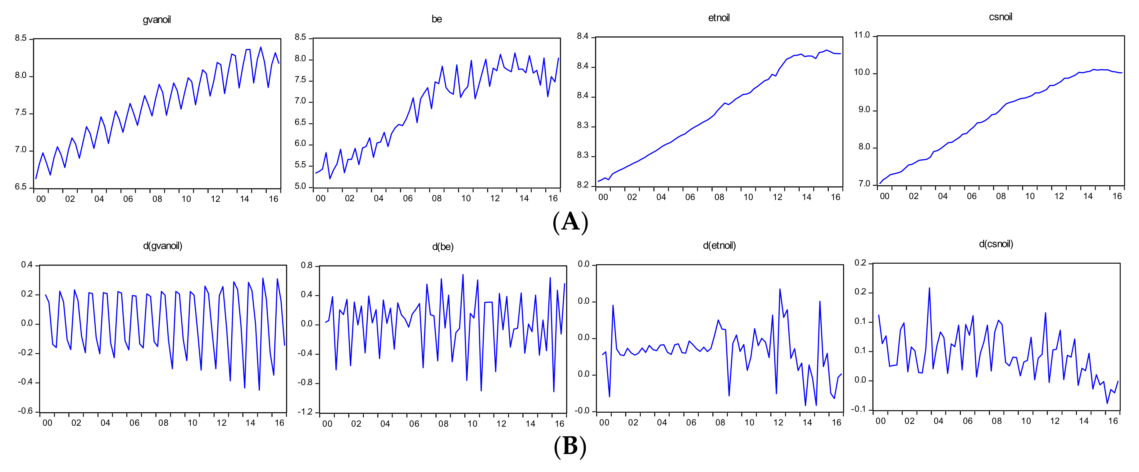
We illustrate the quarterly time profiles of the natural logarithmic expressions of the variables over the period 2000Q1–2016Q4 in Figure 1.
What follows is a brief discussion of the historical development of the variables. As can be seen in panel A, the non-oil value added and government budget expenditures demonstrate seasonality whereas the non-oil capital stock and employment do not. All the three indicators from the non-oil sector here demonstrate a downward shift since 2009, although the seasonality may blur in the non-oil value added. It appears that post-crisis recovery shaped the development trend of the sector so as to be different from what was prevailing before the crisis (Aliyev 2014; Suleymanov and Aliyev 2015). All the variables in panel A share similar movements and display several major events associated with oil-market disruptions. The endogenous reaction of non-oil economic activity to oil-market changes can be attributed to the fact that many non-oil activities are directly or indirectly related to the oil sector. In this regard, all the four variables experienced a sharp decline since 2014, which is caused by the oil-price drop. One important feature of this decline in non-oil economic activity is that it is accompanied by a recession. In the last 17 years, the Azerbaijan economy has never experienced negative growth in two consecutive quarters. However, the sector has seen negative growth in each quarter of the period 2015Q4–2016Q4.
Over the past decade, fiscal policy has been expansionary. Government budget expenditures in nominal terms increased 25 times during 2000–2013, which was enormous, as discussed in the Introduction section. Starting with the oil boom in 2004, the economy enjoyed a decade of oil windfalls, which allowed the government to expand public spending. Public spending from oil revenues has emerged as an important contributor to aggregate demand and growth. Oil revenues (SOFAZ transfers and SOCAR tax payments) accounted for an average of 70% of total budget revenues (30% of GDP) and financed more than half of Azerbaijan’s investment (TAXAZ 2015). However, following the collapse in oil price in 2014, government budget revenues shrank and, consequently, public expenditures declined.
5. Econometric Methods and Strategy for the Empirical Analysis
We explore the impact of fiscal policy on the non-oil sector using the cointegration and error correction modeling framework in this research. The most significant advantage of this framework is that it provides the information set about the long-run relationship and short-run dynamics of the variables as well as the speed of such adjustments from short-term fluctuations to the long-term equilibrium path (Gujarati and Porter 2009, pp. 762–65; Enders 2015, pp. 328–34). Such information is of immense importance both in terms of understanding and policy analysis of the relations between non-oil sector development and its drivers.
We employ the following strategy in our empirical analysis: first, we check unit root (UR) properties of our variables as most of the economic variables are non-stationarity in their level or log-level. For this purpose, we employ the augmented Dickey–Fuller (ADF) unit root test (Dickey and Fuller 1981). To increase the robustness of the results, we also use the Kwiatkowski–Phillips–Schmidt–Shin (KPSS) unit root test (Kwiatkowski et al. 1992). The reason why we prefer the KPSS test to other counterparts as an alternative test is that, unlike other conventional univariate unit root tests, the KPSS takes the null hypothesis of stationarity (or trend stationarity if time trend is included in the test equation). We do not discuss the ADF and KPSS tests here since both of them are widely used in empirical analyses and very well known. A description and discussion of these tests can be found in Dickey and Fuller (1981) and Kwiatkowski et al. (1992) as well as in Enders (2015); Stock and Watson (1993) and Dolado et al. (1990).
Second, if the orders of integration of the variables are the same, then we will check whether they are cointegrated using the Johansen cointegration test (Johansen 1995). We prefer the Johansen test to other cointegration tests such as residual-based developed by Engle and Granger (1987) or single equation-based (e.g., ARDLBT developed by Pesaran et al. 2001) because this is the only test that can discover the number of cointegrated relationships among the variables if the number of explanatory variables is more than one. The point is that other cointegration tests assume that there is only one cointegrating relationship among the variables regardless of how many explanatory variables are included in an analysis. This can cause improper estimations and misleading conclusions. Note that we will also apply a small sample bias correction to the results of the Johansen test to obtain more robust inferences (Reinsel and Ahn 1992; Reimers 1992).
Third, we estimate the parameters of the long-run relationship among the variables if we find cointegration among them. In estimating the long-run coefficients, we will employ the ARDL method by Pesaran and Shin (1998) and Engle–Granger type methods, such as DOLS, FMOLS and CCR along with the Johansen method if we find only one cointegrating relationship among the variables.
Lastly, once the long-run relationship between the variables is estimated and the coefficients obtained, then we will estimate error correction models (ECMs) using the general-to-specific modeling strategy.
Note that the cointegration tests, long-run estimation methods, and ECM that we will employ in this research are comprehensively described and discussed in Section 4.1 in Hasanov et al. (2016). Hence, we do not describe and discuss the aforementioned methods to save space and avoid undue replication and econometric complications.
6. Empirical Results
We document the test and estimation results in this section. Following the strategy given in the previous section, we first report unit root test results. Then we present outcomes of the cointegration test. This is followed by tabulating the long-run estimated coefficients. Finally, we report ECM estimation results.
6.1. Unit Root Test
Table 1 below reports the ADF and KPSS unit root tests results.
The sample values of both tests given in Table 1 suggest that gvanoil, be and etnoil are non-stationary in their level, but stationary in their first difference. For csnoil, the sample values of the ADF and KPSS are again consistent with each other and indicate that the variable is still non-stationary in its first differences. Table 1 shows that the linear trend is still significant in the test equations of both tests when the first differences of the variable, i.e., Δcsnoil are checked. This result is consistent with the graphical illustration of the variable given in Panel B of Figure 1. The test values of the ADF and KPSS on the second difference of the variable, i.e., ΔΔcsnoil are in favor of stationarity. It is worth noting that the formal test results are strongly consistent with the graphical illustrations of the variables given in the panels of Figure 1. Additionally, we illustrate autocorrelation functions (ACF) of the log levels and first differences of the log levels for each variable in Figure A3 in the Appendix, following the recommendation of an anonymous referee. The graphs of ACFs in the figure support the formal unit root test results here.
Thus, the conclusions from the tests are that gvanoil, be and etnoil are I(1) processes while csnoil is an I(2) process.
It is noteworthy that our conclusions for the unit root properties of the non-oil value added, the budget expenditures and non-oil employment are consistent with those found by earlier studies. For example, recent studies such as Hasanov and Alirzayev (2016) and Aliyev et al. (2016) among others also conclude that the variables follow the I(1) process. However, Hasanov et al. (forthcoming) find that non-oil capital stock is a I(1) variable, unlike us. We think that the main reason for obtaining different results for the same variable is the time spans used. Precisely speaking, Hasanov et al. (forthcoming) use annual time period of 1995–2014 while our quarterly period here covers 2000Q1–2016Q4. In other words, that study’s period ends in 2014, while we use data up to 2016 here. If we look at the time profile of csnoil in panel A of Figure 1, it can be observed clearly that the variable has an upward trend until 2014 and a downward trend since then most likely associated with the oil price drop. In other words, the variable contains two different trends in the period 2000–2016. We believe this leads to the series having more than one root. In fact, we run ADF and KPSS on csnoil over the period 2000Q1–2014Q4, which is the same period used in Hasanov et al. (forthcoming). Both tests profoundly indicate that the variable is I(1).4 It should also be noted that the empirical studies frequently find capital stock being an I(2) process. We think this comes from the fact that investment is an I(1) process, which is quite meaningful. Then, the capital stock, which is the accumulation of the investment, will follow an I(2) process.
It would also be interesting to discuss the fact that although our findings for the non-oil value added and budget expenditures are the same as those found by earlier studies, the test specifications used are different as to whether or not they include the time trend. For example, Hasanov and Alirzayev (2016) above, who also use a quarterly time series for the non-oil value added and budget expenditures for the period 2001Q1–2012Q4, also find that the variables are I(1) and their test specifications for both variables include a linear time trend (see Table 1 in that paper) whereas those in this study do not.5 Our explanation for this difference is again the decline in both variables after 2014, caused by the oil price drop, as can be seen in Figure 1A. Precisely speaking, the decline generates a downward trend since 2014 and, therefore, a linear time trend cannot approximate the trajectories of the variables.
6.2. Estimation Results from the Johansen Approach
The results from the unit root exercise conclude that gvanoil, be and etnoil are integrated in order one while csnoil follows the I(2) process. The theory of cointegration postulates that the order of integration of variables in the cointegration analysis should be the same.6 Therefore, we take the levels of the first three variables and the first difference of csnoil, given that difference of all of them will be stationary, as preconditions in the cointegration analysis. As the first step in the Johansen method, a VAR with endogenous variables of gvanoil, be, etnoil and Δcsnoil and exogenous variables of seasonal dummies, intercept and one pulse dummy is specified.7 With regard to setting optimal lag for the VAR, we follow an ascending order, since we have a small number of observations. Precisely speaking, we first estimate our VAR with one lag and check whether or not its residuals have a serial correlation issue. We pay special attention to serial correlation or autocorrelation as they are very key issues in VAR estimation (see: Johansen 1995; Juselius 2006, among others). It appears that only the lag order of five is sufficient to remove serial correlation from the VAR residuals. Note that as a robustness check we also perform lag exclusion and lag order selection criteria tests, and both suggest five lags as an optimal length. Thus, we decided to stick with a five-lag order for our VAR and use this VAR for our next procedures. As the panels A through C and F in Table 2 report, the VAR has good properties as it is stable and its residuals have no issues with serial correlation and heteroscedasticity, although the residuals are not normally distributed. It is well known that the Johansen method is not sensitive to non-normal residuals (see for example, Gonzalo 1994; Lutkepohl 1991; Hubrich 1999).
As a next step of the Johansen method, we perform the cointegration test on the transformed version of the VAR, which is VECM with four lags.8 Despite the fact that the economic drivers are usually represented by the cointegration equation type (c), where an intercept but not trend is included, we report the test results for the all possible combinations of the deterministic regressors in the test equation, i.e., in five test types at the 5% significance level. Panel E in Table 2 documents the results. Evidently from the panel, all the test specifications show almost one cointegrating relationship among the variables. What follows is a brief discussion of the cointegration relationships from these five test equations. Test type (a) assumes that there is no intercept in the long-run relationship, i.e., the autonomous level of the dependent variable is zero. This version is hard to believe as most economic variables have initial values to start with. Moreover, in this option, Δcsnoil has negative and very large coefficient as well as a SoA that is positive, which are against economic and econometric intuition. Since the sample average growth rate of gvanoil is not zero (but 2.05%), we cannot consider test type (b). In type (c), the coefficients on the variables as well as SoA have expected signs although the magnitudes for the coefficients of Δcsnoil and etnoil are large. In type (d), in which time trend is included in the test equation, the coefficient of etnoil alters its sign to negative, which is meaningless. This is also the case for test type (e). Additionally, one should not go for type (e) as none of the variables in the analysis, i.e., gvanoil, be Δcsnoil and etnoil has a quadratic trend. Thus, we stay with test option (c) since it yields more reasonable results compared to other test types. This selection is also in line with the conventional preference of researchers in economics domain as mentioned above. We will investigate this test type in detail below. The trace and maximum eigenvalue statistics and their small sample adjustment values for test type (c) are given in panel F. The results, especially small sample bias corrected values, indicate only one cointegrating relationship among the variables. The long-run numerical values in this specification are reported in panel A of Table 3.
The VEC with the long-run numerical values given in panel A has the following issues:
- (1)
- SoA is −0.06 with the t-statistic of −0.88 meaning that it is very small and statistically insignificant. This highlights two serious issues: (a) the cointegration relationship is not stable; and (b) there is no statistically significant causality running from the explanatory variables to the non-oil value added in the long-run. Both of them are hard to believe as economic theory articulates that, at the very least, capital and labor have certain impacts on output in the long-run.
- (2)
- The magnitudes of the coefficients on capital and labor are very large while that on the budget expenditures is very small. Additionally, the coefficient of the budget expenditures is not statistically significant. These results are not consistent with production function theory as well as the findings of the earlier studies for Azerbaijan (see, for example, Hasanov et al., forthcoming; Hasanov and Alirzayev 2016; Hasanov 2013, among others).
Thus, we need to refine the obtained cointegration results to make them consistent with both economic theory and the stylized facts of the Azerbaijani economy. To this end, we need to investigate all the variables in the analysis. We should start first with the capital stock variable as it follows an I(2) process and possesses a very large coefficient.9 We restrict its coefficient to be zero and see what the restricted long run looks like. The results obtained seem more meaningful and reasonable now as reported in panel B in Table 3 in terms of economic theory and the findings of the earlier studies for Azerbaijan. Precisely speaking:
- (1)
- SoA is −0.35 with the t-statistic of −2.47 meaning that the cointegration relationship is stable now and there is a causality running from the determinants to the non-oil value added in the long-run.
- (2)
- The magnitude of the coefficient on labor decreased about half, while that on the budget expenditures increased drastically, which are what one should expect. Moreover, the coefficient of the budget expenditures is statistically significant now.
Another advantage of the long-run relationship given in panel B compared to the initial one is that now all explanatory variables are weakly exogenous while non-oil value added is not, as documented in panel C. This allows us to proceed to a single equation-based ECM.
As a robustness check, we test unit root properties of the variables but now using a multivariate stationary testing framework. Results presented in panel D of Table 3 show that the sample values of the χ2 reject the null hypothesis of stationarity at the 1% significance level for all four variables. In other words, the variables are non-stationary in their level. These results support those from the univariate unit root tests in Section 6.1.
Thus, as a representation of the long-run relationship between the variables, we use the equation reported in panel B of Table 3 for further purposes.
6.3. Robustness Check for the Long-Run Relationship
In this section, we conduct a robustness check for the long-run relationship obtained from the Johansen approach. Recall that the Johansen cointegration test statistics find that there is no more than one long-run relationship among the variables. This finding allows us to employ ARDLBT as a single-equation-based cointegration method as well as DOLS, FMOS and CCR as residual-based cointegration methods to estimate numerical values of this relationship for comparison purposes. We give priority to the ARDLBT and discuss it in more detail as it outperforms all its counterparts when a sample span is small, which is the case in this research.
We set the maximum lag order as five for each variable in the ARDL estimation, which is consistent with what we did in the Johansen approach. Then, we let the Schwarz information criterion select optimal lag orders for each variable as we have a small number of observations. The selected specification is ARDL(5,0,4,0) for the variables gvanoil, Δcsnoil, etnoil and be, respectively. The specification’s residuals do not have any problem with the serial correlation, non-normality, heteroscedasticity, ARCH effect and mis-specification.10 This specification yields the following long-run elasticities (probabilities in parentheses) for Δcsnoil, etnoil and be, respectively: 0.46(0.49), 4.38(0.00) and 0.19(0.01). Evidently, Δcsnoil is not statistically significant. This result here supports what we found for Δcsnoil in the Johansen approach. It appears that both the methods do not find the variable reasonable to include in the long-run analysis. Hence, we exclude Δcsnoil from the ARDL estimation and re-run it. Table 4 summarizes the ARDLBT estimation and test results.
We set the maximum lag orders for the variables to be five and the Schwarz information criterion selected the ARDL(5,4,0) among 180 rival specifications. The specification successfully passes all the diagnostics and mis-specification tests as presented in panel B. The sample value of F-statistic for the bounds tests of ARDL(5,4,0) suggests that there is a cointegrated relationship among the variables at the 10% significance level regardless of the fact that we use Pesaran et al. (2001) critical values or Narayan (2005) critical values as small-sample bias correction. Panel D reports the numerical values of the long-run relationship derived from ARDL(5,4,0).
Finally, we estimate the numerical values of the long-run relationship also using DOLS, FMOS and CCR as a further robustness check.
Table 5 brings together the estimated long-run elasticities from the five different methods for comparison purposes.
As evidenced from the table, the estimated long-run elasticities from the different methods are very close to each other and they are statistically significant. Only the values from the DOLS are somewhat different from those estimated by the other methods. Most likely it is because the DOLS consumes one lead, which results in the estimation sample ending in 2016Q3 while this is 2016Q4 in the rest of the methods.
It can be concluded that the long-run elasticities of non-oil value added with respect to budget expenditures and non-oil employment are around 0.20 and 5.00, respectively.
6.4. Short-Run Analysis: Error Correction Model (ECM) Estimation
Engle and Granger (1987) discuss that if there is a long-run relation between variables, then there is also an error correction representation of this relation. Furthermore, De Brouwer and Ericsson (1995, 1998) state that if all regressors are weakly exogenous to the long-run relationship, then it is more efficient to use a single equation, rather than a system of equations to model the error correction representation. Both conditions hold in this research, and hence we use a single-equation ECM here.
Although we have long-run elasticities estimated from the five different methods, we used those from ARDL estimation to calculate the error correction term (ECT) for the following two reasons. First, ARDL outperforms all other cointegration methods in the case of small samples; and second, all the elasticities from the different methods are quite close to each other. We include change in Δcsnoil in general/unrestricted ECM alongside changes in gvanoil, etnoil and be. We also include change in DP09Q1 and seasonal dummies in the unrestricted ECM and set the maximum lag order to five.11 Then we try to find a parsimonious ECM through the GtSMS. The final ECM specification and test results are reported in Table 6.
Since the error correction term, ECM_ARDLBT (−1), has a statistically significant coefficient with a negative sign, we can once more confirm that there is a stable cointegrating relationship among the non-oil value added, budget expenditures, non-oil capital and labor. Moreover, panel B of the table show that the residuals of the final specification do not have any problem with the serial correlation, non-normality, ARCH effect, or heteroscedasticity. Furthermore, this shows that the specification is correctly specified.
7. Discussion of the Empirical Results
This section first discusses the unit root and cointegration tests results and then the long-run estimation results. It will be followed by the discussion of the short-run analysis.
Table 1 and Figure 1 both show that the non-oil value added, budget expenditures and non-oil employment follow an integrated process of order one meaning that the log levels of these variables are non-stationary, but their growth rates are stationary. The interpretation of this finding is that mean, variance and covariance of the log levels of the variables change over time in the period considered. Moreover, any sudden changes and interventions to them may have permanent effects. Therefore, it is hard to predict their future values. However, the growth rates of the variables have invariant mean, variance and covariance over time.12 Additionally, they are mean-reverting processes, hence, one should use growth rates of the variables in forecasting future values. When it comes to the non-oil capital stock, one should take its difference twice in order to obtain its stationary condition. Usually, economically, it is hard to interpret the second difference of the log level of the variables. However, the good thing is that for the capital stock, there is an economically reasonable explanation. Precisely speaking, the first difference of the log of the variable will be the investment and the second difference will be the change in the investment.
There is a possibility that the variables share a common trend and move together since they are non-stationary, i.e., they follow unit root process. We call this cointegration, co-movement or a long-run relationship. The results from the Johansen test, reported in Table 2, as well as the ARDLBT test, documented in Table 4 as a robustness check, show that the variables move together in the long run. The cointegration relationship indicates that the variables are related to each other in line with economic theory, although they can deviate from this relationship in the short run. The main causes of these deviations are policy interventions, any kinds of shocks and fluctuations as a result of changes in domestic and international markets.13 However, these deviations from the long-run equilibrium relationship are temporary and will vanish after some time.
The estimated coefficients in Table 5 can be considered as long-run elasticities since we find that there is a long-run relationship between the variables. The table shows that the estimated long-run elasticities from five different estimators are consistent with each other in terms of sign and size. The first three estimators produce very close magnitudes while the CCR and DOLS coefficients are slightly low. Ceteris paribus, a 1% increase in the government budget expenditures will lead to about a 0.2% increase in the value-added of the non-oil sector in the long-run. We will discuss this finding in more detail because the focal point in our study is to explore the non-oil sector growth effects of fiscal policy measured in budget expenditures. The positive impact of fiscal policy is statistically significant at a 1% significance level and consistent with economic theory. The theory, especially Keynesian theory, articulates that government spending can support economic activity and thus boost economic growth. It is not surprising that the economy, including the non-oil sector, is positively affected by government spending. There are some explanations for this finding. First, fiscal policy has a dominant position in the oil-exporting developing countries to drive economic activities. Among other studies, Sturm et al. (2009) for the oil-dependent economies generally and Koeda and Kramarenko (2008); Hasanov (2011) and Dehning et al. (2016) for Azerbaijan in particular discuss how fiscal policy shapes overall policy implementations and how fiscal expansion influences economic growth. Second, the main source of government spending is oil-export revenues and, hence, any changes in oil prices and exports reflect in government spending, as discussed in the Introduction. A number of studies discuss the mechanism of oil-revenue management and show that spending part of the revenues through the government budget is drastically high in Azerbaijan compared to other similar oil-exporting economies (see Wakeman-Linn et al. 2002; Kalyuzhnova and Kaser 2006; Bagirov 2006; Paczynski and Tochitskaya 2008; Sturm et al. 2009; Hasanov and Joutz 2013 and Aliyev et al. 2016). Third, government budget expenditures, particularly capital spending in the form of large-scale infrastructure and social projects, are mainly oriented to non-tradable branches such as construction and service, which are the main parts of the non-oil sector. Hasanov and Alirzayev (2016), using official statistical figures of Azerbaijan, illustrate that the share of capital spending in total budget expenditures was on average more than 30% over 2001–2012 and more than 40% since 2006 when the Baku–Tbilisi–Ceyhan pipeline—the biggest oil-export pipeline of Azerbaijan—started to operate. Aliyev and Mikayilov (2016) discuss how government budget expenditures, hugely financed by the oil revenues, lead to a significant increase in non-tradable branches.
We compare our estimated elasticity of the non-oil value added with respect to government budget expenditures with those of earlier studies for Azerbaijan. Our estimations, which ends in 2016Q4, find the elasticity being 0.20. This is lower than the findings of earlier studies. For example, Hasanov (2013) and Hasanov and Alirzayev (2016) found this elasticity to be around 0.55 and 0.60 for the periods 1998Q4–2012Q3 and 2001Q2–2012Q4, respectively. Gurbanov et al. (2017) estimated it being around 0.40 for 2000Q1–2013Q4. Note that none of the earlier studies employed the production function approach but rather used the specifications, where the non-oil value-added was a function of government budget expenditures and other control variable(s).
Finally, we test whether the small magnitude of our elasticity is due to the low oil prices and can increase if we drop the low oil-price sub-sample in our estimations. To this end, we re-run the estimations until 2014Q1. We find that the magnitude increases and the new coefficients are statistically significant in all estimations. For example, it increases from 0.18 to 0.28 in FMOLS, from 0.13 to 0.22 in DOLS, from 0.16 to 0.27 in CCR, and from 0.21 to 0.23 in ARDL estimations.14
Thus, we think there are two explanations for the question as to why our magnitude of the government budget expenditures effect is small compared to earlier studies. These is a low oil-price environment and a different model specification is used. Evidently, and as discussed in the Introduction, the recent low oil-price environment resulted in a considerable slowdown in the economy including non-oil sector, which has not observed since the 1990s.
As for the short-run effect, we find that the contemporaneous growth rate of government budget expenditures has a positive effect on the growth rate of the non-oil value added by 0.07. Just for the purpose of comparison, note that Hasanov and Alirzayev (2016) found this contemporaneous effect of government budget expenditures to be about 0.15 in the short-run. It appears that the declining effect of the low oil prices holds true also in the short run.
We find that the long-run elasticity of the non-oil value added with respect to non-oil employment is around 5.00, while the net short-run effect of the employment is negative. Both results are consistent with the production function concept articulating that the first order partial derivate of output with respect to labor and capital is positive while the second order partial derivative is negative. In other words, a positive change in employment creates a positive change in output, whereas a positive change in the growth rate of employment is related to a negative change in the growth rate of output.
Furthermore, for the short-run results, we also find that SoA is −0.33. Precisely speaking, if the policy and/or other interventions in the present quarter create a deviation from the long-run relationship between non-oil value-added, employment and government budget expenditures, then 33% of the deviation will be restored back to an equilibrium path in the next quarter. This implies that a whole restoration will take less than one year. The economic interpretation of this finding is that the non-oil value-added is strongly tied to government expenditures. Statistical figures, as well as earlier research, also show that government expenditures are one of the main drivers of non-oil economic development. This is not surprising and a commonly accepted phenomenon for oil-exporting developing/emerging economies.
Finally, and as expected, the non-oil sector was negatively affected by the crisis in 2009, since the dummy variable appears statistically significant in the final ECM specification.
8. Concluding Remarks and Policy Recommendations
This research examines the impact of government budget expenditures on the non-oil sector over a longer period, in which the recent low oil-price sample is incorporated for Azerbaijan.
We underpin the extended production function framework and employ different tests and estimation methods as well as address small-sample bias issues to acquire robust empirical findings.
Findings from the different cointegration methods are close to each other and show that government budget expenditures have a significant positive impact on the non-oil sector both in the long and short runs. However, the magnitude of the effect is small compared to those obtained in earlier studies, because of, we believe, the low oil-prices and different model specifications employed in the empirical analyses. We further find non-oil employment is one of the drivers of non-oil growth.
For Azerbaijani policymakers, the findings show that it is important to think about how to compensate the declining share of oil revenues in total budget revenues. In this regard, the policymakers may think about increasing tax rates, import and export fees, energy and other tariffs as quick remedies to fill the budget. These measures may be successful in the short run but might deter domestic and foreign entrepreneurs, and thus hinder economic development in the medium and longer terms. An alternative and less harmful short-run remedy, we think, would be optimizing government spending. Additionally, the government should also strongly monitor implementation of ongoing projects to increase an efficient usage of revenues. Moreover, the government can phase out social and infrastructure projects, which make lower contributions to valued-added and job creation. Medium- and long-term remedies to increase government revenues may include increasing efficiency in tax collections, improving and facilitating tax and custom legislation, which can lead to more revenue collection, and establishing a favorable environment to attract more foreign direct investment, among others.
Policymakers may think about measures to increase non-oil employment, as it has a positive impact on the development of the non-oil sector.
This research may encourage researchers to examine the relationship in various natural resource-rich economies such as Kazakhstan and Russia, especially when considering the low oil-price environment. In addition, future research may revisit this topic to investigate whether or not the magnitude of the impact of government expenditures on the non-oil sector remains constant or varies over time. Another interesting topic to explore would be the threshold-level of oil prices, in which the impact of government expenditures on the non-oil sector switches from high magnitude to low if this impact is not stable over time.
Acknowledgments
We are grateful to two anonymous referees, and the editors for their comments and suggestions that have helped to improve considerably the paper; nonetheless, we are of course responsible for all errors and omissions. The views expressed in this paper are those of the authors and do not necessarily represent the views of their affiliated institutions.
Author Contributions
Fuad Mammadov gathered data, performed the descriptive analysis. He contributed to the Econometric Methods and Strategy for the Empirical Analysis section and write-up of the Empirical Results section, prepared the References section and made a proof read of the paper. Nayef Al-Musehel did literature review. He also contributed to the write-up of the Empirical Results section and made a proof read of the paper. The rest sections were handled by Fakhri Hasanov.
Conflicts of Interest
The authors declare no conflict of interest.
Appendix A
Figure A1.
Oil revenues as a percentage of total budget revenues *. Source: TAXAZ (2015); SOFAZ (2017) and SSCRA (2017). * We start off in 2003 here and not 2000 because the first publicly available data on oil revenue transfers to the government budget from the State Oil Fund of Azerbaijan, which was operated in 2001, was in 2003 (http://www.oilfund.az/uploads/Annual_Report_2016_AZ.pdf).
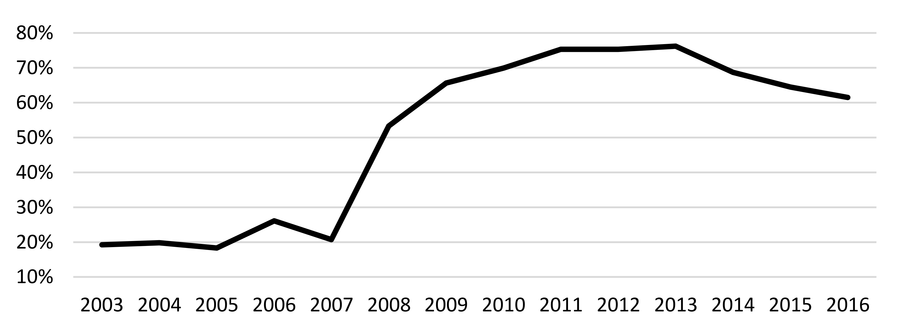
Figure A2.
Relationship between oil prices, government budget expenditures and non-oil value-added * Source: US EIA (2018); SSCRA (2017) and CBAR (2017). * Non-oil value-added is measured in 2010 constant prices by the State Statistical Committee of the Republic of Azerbaijan as indicated in the data section.

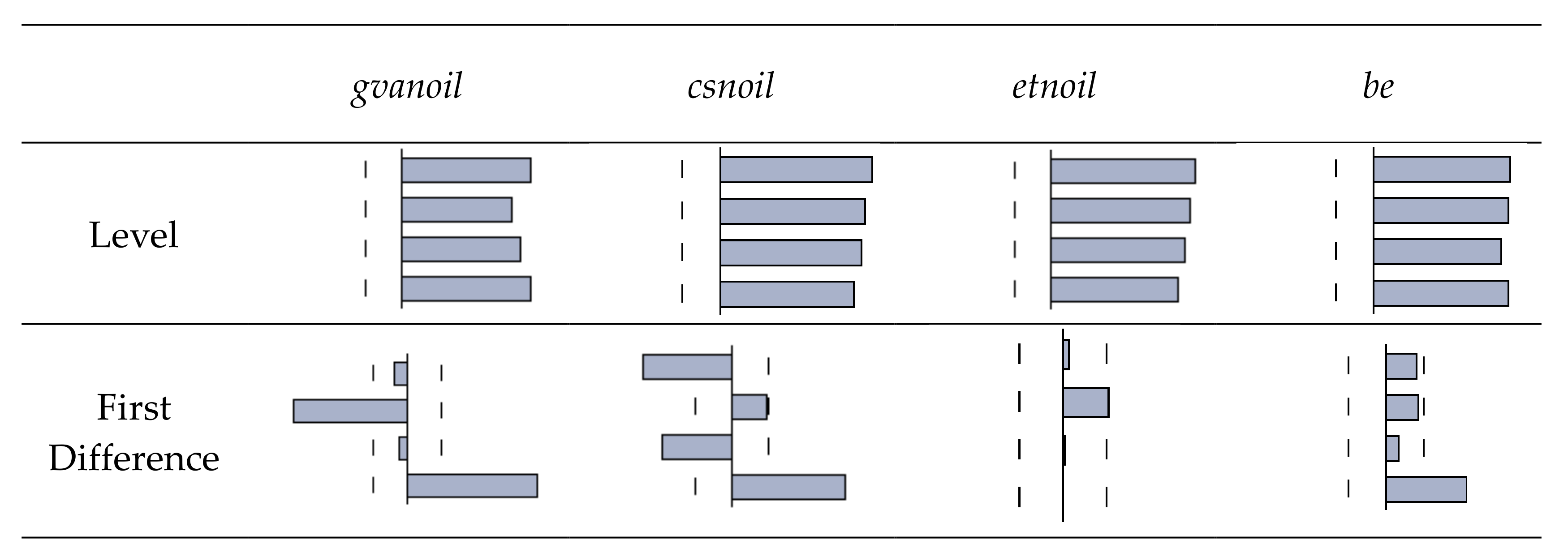
Figure A3.
Graphs of the autocorrelation function of the variables. Note: gvanoil, csnoil, etnoil and be are the logs of value added, capital stock, employment in the non-oil sector and government budget expenditures, respectively.
Figure A3.
Graphs of the autocorrelation function of the variables. Note: gvanoil, csnoil, etnoil and be are the logs of value added, capital stock, employment in the non-oil sector and government budget expenditures, respectively.

References
- Aliyev, Ilkin. 2013. Essays on Natural Resource Impact Center for Economic Research and Graduate Education. dissertation, Charles University, Prague, Czech Republic. Available online: http://www.cerge-ei.cz/pdf/dissertations/2013-aliyev.pdf (accessed on 5 June 2017).
- Aliyev, Khatai. 2014. Expected Macroeconomic Impacts of the Accession to WTO on Azerbaijan Economy: Empirical Analysis, MPRA Paper 55096. Munich: University Library of Munich. [Google Scholar]
- Aliyev, Khatai, and Ceyhun Mikayilov. 2016. Does the Budget Expenditure Composition Matter for Long-Run Economic Growth in a Resource Rich Country? Evidence from Azerbaijan. Academic Journal of Economic Studies 2: 147–68. [Google Scholar]
- Aliyev, Khatai, and Orkhan Nadirov. 2016. How fiscal policy affects non-oil economic performance in Azerbaijan? Academic Journal of Economic Studies 2: 11–29. [Google Scholar]
- Aliyev, Khatai, Bruce Dehning, and Orkhan Nadirov. 2016. Modelling the Impact of Fiscal Policy on Non-Oil GDP in a Resource Rich Country: Evidence from Azerbaijan. Acta Universitatis Agriculturae et Silviculturae Mendelianae Brunensis 64: 1869–78. [Google Scholar] [CrossRef]
- Bagirov, Sabit. 2006. Azerbaijan’s Oil Revenues: Ways of Reducing the Risk of Ineffective Use. Policy Paper. Budapest: Central European University. [Google Scholar]
- Barro, Robert J. 1988. Goverment Spending in a Simple Model of Endogenous Growth. NBER Working Paper No: 2588. Cambridge: National Bureau of Economic Research. [Google Scholar]
- Budina, Nina, Sweder Van Wijnbergen, Zeljko Bogetic, and Smits Karlis. 2010. Long-Term Fiscal Risks and Sustainability in an Oil-Rich Country: The Case of Russia. Washington: World Bank. [Google Scholar]
- Caporale, Guglielmo Maria, and Nikitas Pittis. 1997. Causality and forecasting in incomplete system. Journal of Forecasting 16: 425–37. [Google Scholar] [CrossRef]
- Caporale, Guglielmo Maria, Peter G. Howells, and Alaa M. Soliman. 2004. Stock market development and economic growth: The causal linkages. Journal of Economic Development 29: 33–50. [Google Scholar]
- CBAR. Central Bank of the Republic of Azerbaijan, Statistical Bulletin, October 2017. Available online: https://www.cbar.az/assets/4455/STATISTIK_BULLETEN_2017_OKTYABR.pdf (accessed on 2 October 2017).
- Cobb, Charles Wiggins, and Paul Howard. 1928. A Theory of Production (PDF). American Economic Review 18: 139–65. [Google Scholar]
- Collins, Susan M., Barry P. Bosworth, and Dani Rodrik. 1996. Economic growth in East Asia: Accumulation versus assimilation. Brookings Papers on Economic Activity 1996: 135–203. [Google Scholar] [CrossRef]
- De Brouwer, Gordon, and Ericsson Neil R. 1995. Modeling Inflation in Australia; Research Discussion Paper 9510, International Finance Discussion Paper 530; Sydney, Australia: Reserve Bank of Australia.
- De Brouwer, Gordon, and Ericsson Neil R. 1998. Modeling Inflation in Australia. Journal of Business Economic Statistics 16: 433–449. [Google Scholar] [CrossRef]
- Dehning, Bruce, Khatai Aliyev, and Orkhan Nadirov. 2016. Modelling ‘productivity’ of budget expenditure items before-and-after the oil boom in a resource rich country: Evidence from Azerbaijan. International Journal of Economic Research 13: 1793–806. [Google Scholar]
- Dickey, David, and Wayne Fuller. 1981. Likelihood Ratio Statistics for Autoregressive Time Series with a Unit Root. Econometrica 49: 1057–72. [Google Scholar] [CrossRef]
- Dolado, Juan J., Tim Jenkinson, and Simon Sosvilla-Rivero. 1990. Cointegration and unit roots. Journal of Economic Surveys 4: 249–73. [Google Scholar] [CrossRef] [Green Version]
- Douglas, Paul H. 1976. The Cobb-Douglas Production Function Once Again: Its History, Its Testing, and Some New Empirical Values. Journal of Political Economy 84: 903–16. [Google Scholar] [CrossRef]
- Enders, Wolter. 2015. Applied Econometrics Time Series, Wiley Series in Probability and Statistics, 5th ed. Tuscaloosa: University of Alabama. [Google Scholar]
- Engle, Robert F., and Clive W. J. Granger. 1987. Cointegration and Error-Correction: Representation, Estimation, and Testing. Econometrica 55: 251–76. [Google Scholar] [CrossRef]
- Gonzalo, Jesus. 1994. Five Alternative Methods of Estimating Long-Run Equilibrium Relationships. Journal of Econometrics 60: 203–33. [Google Scholar] [CrossRef]
- Gujarati, Damodar N., and Dawn C. Porter. 2009. Basic Econometrics, 5th ed. Boston: McGraw-Hill. [Google Scholar]
- Gurbanov, Sarvar, Jeffrey B. Nugent, and Jeyhun Mikayilov. 2017. Management of Oil Revenues: Has That of Azerbaijan Been Prudent? Economies 5: 19. [Google Scholar] [CrossRef]
- Hasanov, Fakhri. 2011. Analyzing Price Level in a Booming Economy: The Case of Azerbaijan. Working Paper Series No 11/02E; Kiev: Economics Education and Research Consortium. [Google Scholar]
- Hasanov, Fakhri. 2013. The Role of the Fiscal Policy in the Development of the Non-Oil Sector in Azerbaijan. Hazar Raporu 4: 162–73. [Google Scholar]
- Hasanov, Fakhri, and Elvin Alirzayev. 2016. Is Fiscal Policy Supportive for Non-oil Sector Development: The Case of Azerbaijan, Society of Policy Modeling, EconModels. Working Papers. Available online: http://www.econmodels.com/public/dbArticles.php (accessed on 15 November 2016).
- Hasanov, Fakhri J., and Federick L. Joutz. 2013. A macroeconometric model for making effective policy decisions in the Republic of Azerbaijan. Paper presented at International Conference on Energy, Regional Integration and Socio-Economic Development 6017, Baku, Republic of Azerbaijan, September 5–6. [Google Scholar]
- Hasanov, Fakhri, Ceyhun Mikayılov, Sebuhi Yusifov, and Khatai Aliyev. 2016. Impact of Fiscal Decentralization on Non-Oil Economic Growth in a Resource Rich Economy. Eurasian Journal of Business and Economics 9: 87–108. [Google Scholar] [CrossRef]
- Hasanov, Fakhri J., Cihan Bulut, and Elchin Suleymanov. 2017. Review of Energy-Growth Nexus: A Panel Analysis for Ten Eurasian Oil-Exporting Countries. Renewable & Sustainable Energy Reviews 73: 369–86. [Google Scholar]
- Hasanov, Fakhri, Ceyhun Mikayılov, Sebuhi Yusifov, Khatai Aliyev, and Semra Talishinskaya. forthcoming. The Role of Social and Physical Infrastructure Spending in Development of Tradable and Non-tradable Sectors in Azerbaijan Forthcoming in Contemporary Economics.
- Hubrich, Kirstin. 1999. Estimation of a German Money Demand System: A long-Run Analysis. Empirical Economics 24: 77–99. [Google Scholar] [CrossRef]
- Johansen, Søren. 1995. Likelihood-Based Inference in Cointegrated Vector Auto-Regressive Model. Oxford: Oxford University Press. [Google Scholar]
- Juselius, Katarina. 2006. The Cointegrated VAR Model: Methodology and Applications. New York: Oxford University Press Inc. [Google Scholar]
- Kalyuzhnova, Yelena, and Michael Kaser. 2006. Prudential Management of Hydrocarbon Revenues in Resource-rich Transition Economies. Post-Communist Economies, Taylor & Francis Journals 18: 167–87. [Google Scholar]
- Koeda, Junko, and Vitali Kramarenko. 2008. Impact of Government Expenditure on Growth: The Case of Azerbaijan, IMF Middle East and Central Asia Department, WP/08/115. Available online: www.imf.org/external/pubs/ft/wp/2008/wp08115.pdf (accessed on 24 April 2017).
- Kwiatkowski, Denis, Peter C. B. Phillips, Peter Schmidt, and Yongcheol Shin. 1992. Testing the null hypothesis of stationarity against the alternative of a unit root. Journal of Econometrics 54: 159–78. [Google Scholar] [CrossRef]
- Lucas, Robert E. 1988. On the Mechanics of Economic Development. Journal of Monetary Economics 22: 3–42. [Google Scholar] [CrossRef]
- Lutkepohl, Helmut. 1982. Non-causality due to omitted variables. Journal of Econometrics 19: 367–78. [Google Scholar] [CrossRef]
- Lutkepohl, Helmut. 1991. Introduction to Multiple Time Series. New York: Springer, 552p, ISBN 0-387-53194-7. [Google Scholar]
- MacKinnon, James. 1996. Numerical Distribution Functions for Unit Root and Cointegration Tests. Journal of Applied Econometrics 11: 601–18. [Google Scholar] [CrossRef]
- MacKinnon, James G., Alfred H. Alfred, and Michelis Leo. 1999. Numerical distribution functions of likelihood ratio tests for cointegration. Journal of applied Econometrics 14: 563–77. [Google Scholar] [CrossRef]
- Michael, Berlemann, and Jan-Erik Wesselhöft. 2014. Estimating aggregate capital stocks using the perpetual inventory method: A survey of previous implementations and new empirical evidence for 103 countries. Review of Economics 65: 1–34. [Google Scholar]
- Narayan, Paresh Kumar. 2005. The saving and investment nexus for China: Evidence from cointegration tests. Applied Economics 37: 1979–90. [Google Scholar] [CrossRef]
- Nehru, Vikram, and Ashok Dhareshwar. 1993. A new database on physical capital stock: Sources, methodology and results. Revista de Análisis Económico 8: 37–59. [Google Scholar]
- Odhiambo, Nicholas M. 2008. Financial depth, savings and economic growth in Kenya: A dynamic causal relationship. Economic Modeling 25: 704–13. [Google Scholar] [CrossRef]
- Odhiambo, Nicholas M. 2009. Electricity consumption and economic growth in South Africa: A trivariate causality test. Energy Economics 31: 635–40. [Google Scholar] [CrossRef]
- Paczynski, Wojciech, and Irina Tochitskaya. 2008. Economic Aspects of the Energy Sector in CIS Countries. (CASE 34 for DG ECFIN/D/2007/005). Moscow: European Comision. [Google Scholar]
- Pesaran, M. Hashem, and Yongcheol Shin. 1998. An Autoregressive Distributed Lag Modeling Approach to Cointegration Analysis. Econometric Society Monographs 31: 371–413. [Google Scholar]
- Pesaran, M. Hashem, Yongcheol Shin, and Richard J. Smith. 2001. Bound Testing Approaches to the Analysis of Level Relationships. Journal of Applied Econometrics 16: 289–326. [Google Scholar] [CrossRef]
- Reimers, Hans-Eggert. 1992. Comparisons of tests for multivariate cointegration. Statistical Papers 33: 335–59. [Google Scholar] [CrossRef]
- Reinsel, Gregory C., and Sung K. Ahn. 1992. Vector autoregressive models with unit roots and reduced rank structure: Estimation, likelihood ratio test, and forecasting. Journal of Time Series Analysis 13: 353–75. [Google Scholar] [CrossRef]
- SOFAZ. 2017. State Oil Fund of Azerbaijan Republic. Reports and Statistics. Available online: http://www.oilfund.az/en_US/hesabatlar-ve-statistika/hesabat-arxivi.asp (accessed on 19 November 2017).
- Solow, Robert M. 1969. Growth Theory: An Exposition. Oxford: Clarendon Press. [Google Scholar]
- Solow, Robert M. 1988. Growth Theory and After. American Economic Review 78: 307–17. [Google Scholar]
- Sorsa, Piritta. 1999. Algeria-The Real Exchange Rate, Export Diversification, and Trade Protection. Washington: Policy Development and Review Department, International Monetary Fund. [Google Scholar]
- SSCRA. 2017. State Statistical Committee of the Republic of Azerbaijan. Available online: https://www.stat.gov.az/?lang=az (accessed on 5 May 2017).
- Stock, James H., and Mark W. Watson. 1993. A simple estimator of cointegrating vectors in higher order integrated systems. Econometrica: Journal of the Econometric Society 1: 783–820. [Google Scholar] [CrossRef]
- Sturm, Michael, Francois J. Gurtner, and Juan Gonzalez. 2009. Fiscal Policy Challenges in Oil-Exporting Countries a Review of Key Issues Occasional Paper Series No. 104. Frankfurt: European Central Bank. [Google Scholar]
- Suleymanov, Elchin, and Khatai Aliyev. 2015. Macroeconomic Analysis and Graphical Interpretation of Azerbaijan Economy in 1991–2012. Expert Journal of Economics 3: 40–49. [Google Scholar]
- TAXAZ. 2015. Tax System of the Republic of Azerbaijan, Ministry of Taxes, Special ed. Baku: TAXAZ. [Google Scholar]
- Triacca, Umberto. 1998. Non-causality: The role of the omitted variables. Economics Letters 60: 317–20. [Google Scholar] [CrossRef]
- US EIA. 2018. United States Energy Information Agency. Spot Prices for Crude Oil and Petroleum Products. Available online: https://www.eia.gov/dnav/pet/pet_pri_spt_s1_a.htm (accessed on 13 January 2018).
- Wakeman-Linn, John, Paul Mathieu, and Bert Selm. 2002. Oil Funds and Revenue Management in Transition Economies: The Cases of Azerbaijan and Kazakhstan. Washington: IMF. [Google Scholar]
- Wijnbergen, S. Van. 2008. The Permanent Income Approach in Practice: A Policy Guide to Sustainable Fiscal Policy in Azerbaijan. Washington: World Bank. [Google Scholar]
- Zermeno, Mayra. 2008. Current and Proposed Non-Oil Tax System in Azerbaijan IMF Working Paper. Washington: IMF. [Google Scholar]
| 1 | In this research, we do not explore how different components of government expenditure can impact different sub-sectors of the non-oil sector such as tradable and non-tradable branches. |
| 2 | One can think about considering Azeri light oil price instead of using Brent Spot Price for crude oil. However, the point is that first, we could not find historical time series of Azeri light for the quarterly period undertaken in this research and second, the former one very closely follows the latter one. |
| 3 | Hasanov and Alirzayev (2016) discuss the fact that earlier studies by international agencies, such as the International Monetary Fund and World Bank as well as individual researchers also find that the CPI is a more relevant price measure than the GDP deflator to rescale budget expenditures. |
| 4 | The tests results can be obtained from the authors upon request. |
| 5 | We cannot compare our unit root test specifications with those from Aliyev et al. (2016) as they not discuss whether the time trend appears significant/insignificant in their unit root test exercises. |
| 6 | Note, however, that an I(0) variable can be included in the cointegration analysis, where the rest of the variables are I(1) if one employs the Johansen or ARDLBT methods. |
| 7 | We include seasonal dummy variables in the VAR because gvanoil and be demonstrate seasonality, as can be clearly seen in Figure 1. The time trend as a deterministic exogenous variable was also included; however, it was statistically insignificant and additionally led to instability of the VAR. We include a dummy variable, having unity in 2009Q1 and zero otherwise, to capture the effect of the recent financial crisis. If we look at the seasonally adjusted time series of gvanoil, one can probably think about including another pulse dummy variable for the 2015Q4 to capture the consequences of the recent oil-price drop. However, it turns out that this dummy variable causes an instability of the VAR and hence we excluded it. |
| 8 | As Juselius (2006) describes, the proper way of transforming a VAR to a VEC is that if there is for example, a pulse dummy in the former, then a blip dummy should be in the latter. In other words, deterministic variables also should be differenced. Moreover, Johansen (1995) and Juselius (2006) discuss the fact that pulse (blip) dummies do not distort the distribution of the critical values of the cointegration tests. In fact, the test results given in panels E and F do not change at all if we exclude the dummy variables from the test. |
| 9 | Note that we also tried to restrict the coefficients of the budget expenditures and labor being zero separately. Moreover, we checked whether the constant return to scale hypothesis can hold by equaling the sum of the coefficients of the explanatory variables at unity. However, none of these remedies produced something meaningful. |
| 10 | We do not report the residual test results as this ARDL is not the final one. However, the results can be obtained from the authors upon request. |
| 11 | We also initially included a dummy variable to capture a slowdown in non-oil value added caused by the recent oil-price drop as we did in the VAR/VEC analysis above. However, this caused the residuals of the final ECM specification to be heteroscedastic, and led to instability in the VAR analysis. Hence, we excluded it from the ECM analysis. |
| 12 | In economics we have relatively time-invariant mean, variance and covariance which is called weak stationarity (see Gujarati and Porter (2009), among others). |
| 13 | Note that analyzing shock effects, such as the shocks of government budget expenditures and or oil prices on non-oil GDP is out of the scope of this research as our main objective is to examine the long- and short-run impacts of government budget expenditures on the non-oil sector for a more recent period. However, this is an interesting research question and we will consider it in future research. |
| 14 | Note that we do not report the estimations results here to conserve space, but they are available from the authors. |
Figure 1.
Time profiles of the variables. (panel A) Time profiles of the log levels of the variables; (panel B) Time profiles of the first difference of the log levels of the variables. Note: gvanoil, etnoil, csnoil and be are the logs of value added, employment and capital stock in the non-oil sector and the budget expenditures, respectively; d is the difference operator.


Table 1.
The unit root (UR) test results.
| Variable | ADF Test | KPSS Test | |||||||
|---|---|---|---|---|---|---|---|---|---|
| Test Value | C | t | None | k | Test Value | C | t | None | |
| gvanoil | −2.50 | x | 4 | 0.16 ** | x | x | |||
| csnoil | −1.65 | x | 4 | 0.24 *** | x | x | |||
| etnoil | −1.53 | x | 0 | 0.12 * | x | x | |||
| be | −2.01 | x | 4 | 0.25 *** | x | x | |||
| gvanoil | −2.89 * | x | 3 | 0.23 | x | ||||
| csnoil | −2.47 | x | x | 4 | 0.20 ** | x | x | ||
| etnoil | −4.08 *** | x | 1 | 0.31 | x | ||||
| be | −4.14 *** | x | 3 | 0.13 | x | ||||
| csnoil | −12.73 *** | x | 3 | 0.10 | x | ||||
Notes: gvanoil, csnoil, etnoil and be are the logs of value added, capital stock, employment in the Non-oil sector and the government budget expenditures, respectively; Δ is the first difference operator; ADF and KPSS denote the Augmented Dickey-Fuller and Kwiatkowski-Phillips-Schmidt-Shin tests, respectively. Maximum lag order is set to four and optimal lag order (k) is selected based on the Schwarz criterion in the tests; ***, ** and * indicate rejection of the null hypotheses of having unit root in the ADF and stationarity (or trend stationarity) in the KPSS at the 1%, 5% and 10% significance levels, respectively; The critical values for the ADF and KPSS tests are taken from MacKinnon (1996) and Kwiatkowski et al. (1992), respectively. Estimation period: 2000Q1–2016Q4. None means that neither intercept nor trend is included in test equation. Note that final Unit Root test equation can include one of the three: intercept (C), intercept and trend (t) and none of them (None). x indicates that the corresponding option is selected in the final Unit Root test equation.
Table 2.
The vector autoregression (VAR) residual diagnostics and cointegration tests results.
| Panel A: Serial Correlation LM Test a | Panel E: Johansen Cointegration Test Summary | ||||||||
| Lags | LM-Statistic | p-Value | Data Trend: | None | None | Linear | Linear | Quadratic | |
| 1 | 13.39 | 0.64 | Test Type: | (a) No C&t | (b) C | (c) C | (d) C&t | (e) C&t | |
| 2 | 12.41 | 0.72 | Trace: | 1 | 1 | 1 | 1 | 1 | |
| 3 | 25.90 | 0.06 | Max-Eig: | 1 | 1 | 1 | 1 | 2 | |
| Panel B: Normality Test b | Panel F: Johansen Cointegration Test Results for Type c | ||||||||
| Statistic | d.f. | p-Value | Null Hypothesis: | r = 0 | r ≤ 1 | r ≤ 2 | |||
| Skewness | 20.04 | 4 | 0.00 | λtrace | 69.55 *** | 28.30 * | 13.02 | ||
| Kurtosis | 4.33 | 4 | 0.36 | λtrace a | 47.11 * | 19.17 | 8.82 | ||
| Jarque-Bera | 24.38 | 8 | 0.00 | λmax | 41.25 *** | 15.28 | 7.20 | ||
| λmax a | 27.94 * | 10.35 | 4.88 | ||||||
| Panel C: Heteroscedasticity Test c | |||||||||
| White | d.f. | p-Value | |||||||
| Statistic | 459.3 | 440 | 0.25 | ||||||
| Panel D: Stability Test d | |||||||||
| Modulus | Root | ||||||||
| 0.99 | 0.99 + 0.04i | ||||||||
| 0.99 | 0.99 − 0.04i | ||||||||
| 0.97 | −0.98 | ||||||||
| 0.96 | −0.03 + 0.96i | ||||||||
Note: a The null hypothesis in the serial correlation LM test is that there is no serial correlation at lag order h of the residuals; b System normality tests with the null hypothesis of the residuals are multivariate normal; c White heteroscedasticity test takes the null hypothesis of no cross terms heteroscedasticity in the residuals; d VAR stability test results show that no roots of polynomial characteristic are outside the unit circle; is chi-squared; d.f. means degree of freedom; C and t indicate intercept and trend. r is rank of matrix, i.e., number of cointegrated equations; λtrace and λmax are the trace and max-eigenvalue statistics, while λtrace a and λmax a are adjusted version of them; *** and * denotes rejection of null hypothesis at the 1% and 10% significance levels, respectively; Critical values for the cointegration test are taken from MacKinnon et al. (1999); Estimation period: 2001Q3–2016Q4.
Table 3.
The significance, stationarity, weak exogeneity and hypothesis testing results.
| Panel A: Long-Run Equation () | ||||||
| gvanoil = −60.56 + | 6.79 Δcsnoil + | 8.11 etnoil + | 0.04 be + e | |||
| (1.17) | (1.24) | (0.07) | ||||
| Panel B: Long-Run Equation, When | ||||||
| gvanoil = −33.91 + | 4.83 etnoil + | 0.18 be + e | ||||
| (0.83) | (0.05) | |||||
| Panel C: Weak Exogeneity Test Results a | ||||||
| gvanoil | Δcsnoil | etnoil | be | |||
| t-statistic | −2.47 ** | 0.21 | −0.33 | 1.40 | ||
| Panel D: Multivariate Statistics for Testing Stationarity b | ||||||
| gvanoil | Δcsnoil | etnoil | be | |||
| χ2 (1) | 34.40 *** | 15.45 *** | 34.85 *** | 34.40 *** | ||
Notes: gvanoil, csnoil, etnoil and be are the logs of the value added, capital stock, employment in the non-oil sector and government budget expenditures; is the first difference operator; a the null hypothesis is that given variable is weakly exogenous; b the null hypothesis is that given variable is (trend) stationary; *** and ** denote rejection of the null hypotheses at the 1% and 5% significance levels, respectively; values in parentheses are standard errors. Estimation period: 2001Q3–2016Q4.
Table 4.
The autoregressive distributed lagged bound testing (ARDLBT) estimation and test results.
| Panel A: ARDL Specifications: | |||||||
| Specification with optimal lags, ARDL(5,4,0): | |||||||
| Panel B: Residual Diagnostics and Mis-Specification Tests Results for ARDL(5,4,0): | |||||||
| = 6.33 [0.19] | = 2.46 [0.29] | = 15.88 [0.39] | = 3.58 [0.17] | = 0.02 [0.89] | |||
| Panel C: Cointegration Test Results for ARDL(5,4,0): | |||||||
| The sample F-statistic | Significance level | Pesaran et al. (2001) critical values | Narayan (2005) critical values | ||||
| Low bound | Upper bound | Low bound | Upper bound | ||||
| FW = 3.64 | 1% | 4.13 | 5.00 | 4.56 | 5.59 | ||
| 5% | 3.10 | 3.87 | 3.29 | 4.07 | |||
| 10% | 2.63 | 3.35 | 2.74 | 3.47 | |||
| Panel D: Long-Run Relation Derived from ARDL(5,4,0): | |||||||
| gvanoil = −27.49 + | 4.05 etnoil + | 0.21 be + e | |||||
| (1.21) | (0.07) | ||||||
Notes: gvanoil, etnoil and be are the logs of the value added, employment in the non-oil sector and government budget expenditures, respectively; , denote chi-squared statistics to test the null hypotheses of no serial correlation, no autoregressive conditioned heteroscedasticity, and no heteroscedasticity in the residuals; and indicate Jarque–Bera and F-statistic to test the null hypotheses of normal distribution and no functional mis-specification respectively; FW is the F-value of testing the null hypothesis of in the Wald test. Critical values are taken from the case of restricted intercept and no trend, 2 regressors and 62 observations (See: Pesaran et al. 2001, p. 300; Narayan 2005, p. 1987). Probabilities are in brackets and standard errors are in parentheses; the pulse dummy variable of DP09Q1 and seasonal dummies are included in the estimation. Estimation period: 2001Q3–2016Q4.
Table 5.
Long-run elasticities from the methods.
| Methods | etnoil | be | Intercept |
|---|---|---|---|
| Coef. (Std. Er.) | Coef. (Std. Er.) | Coef. (Std. Er.) | |
| VECM | 4.83 *** (0.83) | 0.18 ** (0.05) | −33.91 *** (6.50) |
| ARDLBT | 4.05 *** (1.21) | 0.21 *** (0.07) | −27.49 *** (9.69) |
| FMOLS | 4.86 *** (0.44) | 0.18 *** (0.03) | −34.22 *** (3.50) |
| CCR | 5.29 *** (0.56) | 0.16 *** (0.04) | −36.87 *** (4.39) |
| DOLS | 5.81 *** (0.68) | 0.13 *** (0.04) | −41.75 *** (5.42) |
Notes: The dependent variable is gvanoil; gvanoil, etnoil and be are the logs of the value added, employment in the non-oil sector and the budget exenditures; Coef and Std. Er. mean coefficient and standard error; ** and *** indicate significance levels at 5% and 1%. The pulse dummy variable of DP09Q1 is included in the fully modified ordinary least squares (FMOLS) and canonical cointegrating regression (CCR) estimations while it is insignificant in the DOLS. Estimation period: 2001Q3–2016Q4. Dynamic ordinary least squares (DOLS).
Table 6.
Final error correction model (ECM) specification.
| Panel A: Estimated Coefficients of the Final ECM Specification | |||||||||||
| Reg. | |||||||||||
| Coef. | −0.02 | −0.33 | 0.68 | −6.26 | 4.29 | −4.49 | 0.07 | −0.05 | −0.01 | 0.06 | −0.07 |
| P-val. | 0.28 | 0.00 | 0.00 | 0.00 | 0.04 | 0.02 | 0.01 | 0.10 | 0.89 | 0.02 | 0.01 |
| Panel B: Residuals Diagnostics and Misspecification Tests Results | |||||||||||
| Statistic | FFF | ||||||||||
| Sample value | 0.35 | 0.69 | 1.85 | 2.17 | 2.43 | ||||||
| p-value | 0.28 | 0.41 | 0.08 | 0.34 | 0.13 | ||||||
Notes: Reg., Coef. and p-val. mean regressor, coefficient and probability value to reject given null hypothesis; gvanoil, etnoil and be are the value added, employment in the Non-oil sector and the budget exenditure; c is the intercept; denotes the first difference operator; dependent variable is ; ECT is the error correction term, i.e., one period lagged residuals from the long-run ARDL estimation; denote F statistics to test the null hypotheses of no serial correlation, no autoregressive conditioned heteroscedasticity, no heteroscedasticity in the residuals and no functional form mis-specification, respectively; indicates the Jarque–Bera statistic to test the null hypotheses of normal distribution of the residuals. Estimation period: 2001Q3–2016Q4.
© 2018 by the authors. Licensee MDPI, Basel, Switzerland. This article is an open access article distributed under the terms and conditions of the Creative Commons Attribution (CC BY) license (http://creativecommons.org/licenses/by/4.0/).
Share and Cite
MDPI and ACS Style
Hasanov, F.; Mammadov, F.; Al-Musehel, N. The Effects of Fiscal Policy on Non-Oil Economic Growth. Economies 2018, 6, 27. https://doi.org/10.3390/economies6020027
AMA Style
Hasanov F, Mammadov F, Al-Musehel N. The Effects of Fiscal Policy on Non-Oil Economic Growth. Economies. 2018; 6(2):27. https://doi.org/10.3390/economies6020027
Chicago/Turabian StyleHasanov, Fakhri, Fuad Mammadov, and Nayef Al-Musehel. 2018. "The Effects of Fiscal Policy on Non-Oil Economic Growth" Economies 6, no. 2: 27. https://doi.org/10.3390/economies6020027
Note that from the first issue of 2016, this journal uses article numbers instead of page numbers. See further details here.