Exchange Rate and Oil Price Interactions in Selected CEE Countries

Faculty of Economic Sciences, University of Warsaw, 00-241 Warsaw, Poland
Economies 2018, 6(2), 31; https://doi.org/10.3390/economies6020031
Submission received: 5 November 2017
/
Revised: 23 April 2018
/
Accepted: 4 May 2018
/
Published: 14 May 2018
(This article belongs to the Special Issue Falling Oil Prices: Economic and Financial Implications)
Abstract
:This paper reports a study on the causal dynamics between spot oil price, exchange rates, and stock prices in Poland, the Czech Republic, Hungary, Romania, and Serbia. The results are compared with a benchmark analysis in which U.S. monthly data are used, and time periods are selected according to the flexibility of exchange rate regimes in each country. A period between 2000 and 2015 is analyzed. The methodology is based on the Granger causality test, and the non-linear Diks–Panchenko test, while the causality in variance is checked with the Hafner–Herwartz test.
Keywords:
causality; exchange rates; non-linear causality; oil price; stock prices; volatility spilloverJEL Classification:
C32; C53; E37; F31; F37; G171. Introduction
Recently there was much research devoted towards the analysis of links between oil price and stock prices. There were also speculation that the oil price increase around 2008 was due to the increasing financialization of this market. Oil price changes might also impact economic activity, and therefore, stock markets. For example, Asteriou and Bashmakova (2013) concluded that CEE (Central and Eastern Europe) stock prices respond negatively to positive impacts from the oil price.
Additionally, financial markets are becoming more and more globalized. Therefore, researchers focus on links between stock markets in the international context. From an (foreign) investors’ perspective, the expected returns are determined by both stock prices and exchange rates. As a result, the linkages between exchange rates and stock prices are an important topic in the global context. As one example, this is important in portfolio management, etc. (Abdelaziz et al. 2008). However, the literature is usually divided into two streams of investigations. The first is focused on the relationship between oil price and stock prices. The second, between oil price and exchange rates. It is therefore interesting to focus on the dynamic interactions, simultaneously capturing the behavior of all three of these variables.
Although a few CEE countries have adopted the euro quite recently, most of the CEE countries still use their own currency. Such countries include Poland, the Czech Republic, Hungary, Romania, Bulgaria, Croatia, Serbia, Bosnia and Herzegovina, the Republic of Macedonia, and Albania.
In Poland there has been a free floating exchange rate regime since 2000. In Czech Republic there has been a managed floating regime since 1997, but since 2002 no direct intervention of the Czech National Bank had occured until 2013, so in practice a free float regime can be assumed until then. In 2014, the International Monetary Fund (IMF) classified the Hungarian forint and Romanian leu as floating currencies, although they are not strictly free floating.
In this context it is important to notice that: “There is no consensus concerning the existence of a clean or free floating regime. Most authors, however, do believe that free floating is the only theoretical solution because in practice intervention is always present; having in mind that the exchange rate is the most important price in an open economy, which simultaneously influences internal and external balances. The main point is only how frequent and how strong intervention is, and whether it is planned or ad hoc” (Josifidis et al. 2009).
For Romania until 2005, a managed float can be assumed, but must be abandoned in later years. In Hungary, since 2001 a certain crawling peg has existed, but with increasingly wide bands. Floating has existed since 2008 there. Serbia (since 2009) has had a managed float exchange regime, sometimes classified as just floating. In the case of a managed float regime, the exchange rate can fluctuate, but a central bank has certain policies to influence the rate. In 1992, Albania (with a currency called lek) adopted free floating. On the other hand, the Bulgarian lev and Croatian kuna are fixed to the euro. Bosnia and Herzegovina’s convertible mark and Macedonia’s denar are also, in practice, pegged to the euro. Nevertheless, it seems that most of the CEE countries with soft pegs gradually increase the flexibility of their currencies (Belke and Zenkic 2007; Causevic 2015; IMF 2009, 2015; Mirdala 2013).
Of course, CEE countries are not large economies, nor are they top oil exporters or importers. According to the EIA (U.S. Energy Information Administration), Poland is the 15th oil exporter, Hungary is 22nd, and the Czech Republic is 24th out of a list of 25 countries. In terms of a list of 30 oil importers, Poland is 13th, the Czech Republic is 22nd, and Hungary is 24th. In case of production, Romania is the 48th world petroleum producer, Poland is 65th, Hungary is 72nd, Albania and Serbia are equally 74th, Croatia is 81st, the Czech Republic is 89th, and Bulgaria is 100th, where the ranking consists of 117 countries. In terms of consumption, Poland is 32nd, Czech Republic and Romania are equally 59th, Hungary is 68th, Bulgaria is 80th, Croatia is 83th, Serbia is 85th, and Albania is 117th out of 213 countries listed (EIA 2015).
CEE economies are also quite vulnerable to energy use. According to World Bank (2015), the GDP per unit of energy use is 5.3 (PPP USD/kg oil equivalent) in Bosnia and Herzegovina, 6.2 in Bulgaria and Serbia, 7.0 in the Czech Republic, 8.8 in Poland, 9.4 in Hungary, 10.1 in Romania, and 10.9 in Croatia. Energy use in kg of oil equivalent per capita varies from 1742 in Bosnia and Herzegovina to 4057 in the Czech Republic (World Bank 2015). These indicators clearly show that CEE economies are dependent on energy in a more similar pattern to developed countries, than to the developing ones. Moreover, the trend is continuing as their economies become more developed.
Therefore, it is interesting to examine the oil price–exchange rates relationship for CEE countries. These countries have recently become interesting for various investors. Their linkages with developed Western European countries are expanding. Moreover, these countries are becoming a target for various industry sectors (i.e., energy consuming ones) in the case of factory locations, etc. In 2013, the net FDI (foreign direct investment) to CEE countries was 6501 mln EUR. Over 2600 mln EUR was invested in Romania and almost 1300 mln EUR in the Czech Republic (Popescu 2014).
Moreover, net inflows of private capital as a percentage of GDP in CEE countries is significantly higher than in all of the world’s emerging markets (Mihaljek 2009). As a result, these economies can increase their dominance in the international landscape in the near future. It is also interesting to compare the behavior of emerging economies with developed ones for basic scientific reasons. For example, the recent global financial crisis showed that their reaction can be a bit different.
Finally, economic growth is linked with the energy consumption (Mucuk and Sugozu 2011). Therefore, oil price interaction with the exchange rate is an important topic from the emerging economies point of view. Indeed, such information is crucial for long-term energy policies.
2. Literature Review
Hamilton (2003) and Kilian (2006 suggested that oil price shock can significantly affect various macroeconomic factors. This influence can be both linear and non-linear (Bal and Rath 2015; Beckmann and Czudaj 2013). One of the well-known explanations for why oil price shock can influence exchange rates is given by Golub (1983). An oil price shock can start a wealth transfer from an oil importing country to an oil exporting country, and, consequently imply changes in the exchange rate. This can also be influenced through changes in terms of trade and net foreign assets. Therefore, the exchange rate regime is an important factor (Bodart et al. 2015; Broda 2004; Ilzetski et al. 2017). In the other direction, an appreciation of a domestic currency against the currency in which oil is denominated, lowers the oil price expressed in the domestic currency. This results in a demand increase and can further result in an oil price increase (Akram 2009).
The relationship between exchange rate and oil price is a topic of various research, both in the case of developed and developing economies. However, it is often examined just in the case of the EUR/USD exchange rate (Aloui et al. 2013; Ciner et al. 2013; Ding and Vo 2012; Ferraro et al. 2015; Novotny 2012; Zhang et al. 2008). Alternatively, a certain weighted currency index vs. USD can be used. For example, Basher et al. (2012) used the Federal Reserve Board trade weighted exchange index for major traded currencies index (TWEXMMTH). Such an approach loses information about a particular country.
Brahmasrene et al. (2014) found that there exists a Granger causality from exchange rates to oil price in the short-term. Moreover, there is a causality from oil price to exchange rates in the long-term. They also found that exchange rate shock has a significant negative impact on oil price, but its impulse response is not significant. Bi-directional causality was also studied, for example, by Al-Mulai and Sab (2011), Huang and Tseng (2010), and Mohammadi and Jahan-Parvar (2010).
In the case of CEE economies this link has not been explored so intensively. However, for other post-communist transition economies there is an interesting literature (Habib and Kalamova 2007; Fakhri 2010; Fakhri et al. 2017; Kalcheva and Oomes 2007). Moreover, Reboredo (2012) stated that although oil price and exchange rates were not significantly correlated, their interdependence significantly grew since the beginning of the recent global financial crisis. Similar conclusions were drawn by Reboredo and Rivera-Castro (2013). Additionally, Turhan et al. (2013) considered daily time-series for selected emerging markets and concluded that an increase in oil price results in the appreciation of an emerging economy’s currency. This relationship is more evident since 2008. Brahmasrene et al. (2014) also stressed the impact of high price volatility in this period.
On the other hand, Uddin et al. (2013) argued that the relationship between exchange rates and oil price is still ambiguous, and, moreover, the strength of this relationship changes over time. Beirne and Bijsterbosch (2011) examined nine of the CEE countries in order to check the exchange-rate pass-through (i.e., the elasticity of local currency import prices with respect to the local currency price of a foreign currency). It was found to be between 0.5 and 0.6. However, in the present context, the most important fact is that a significant cointegration between exchange rates was found. Indeed, the recent research of Andries et al. (2016) suggests that in the short-term and medium-term exchange rates in CEE countries are highly integrated. On the other hand, for times longer than six months, significant discrepancies are observed.
Basher et al. (2012) applied VAR (vector auto regression) models to study the relationship between oil price, stock prices, and exchange rates in emerging economies. They found that positive shocks to oil price can result in a decrease of stock prices on emerging markets in the short-term. However, their research did not focus on particular CEE countries, but rather on big emerging economies like Brazil, China, or other Asian countries (Narayan 2013). Tiwari et al. (2013) argued that oil price influences the real effective exchange rate both in the short-term and long-term.
Ghosh (2011) found that an increase in oil price results in the depreciation of Indian currency to USD. According to the applied E-GARCH methodology no asymmetric impact was found, i.e., positive and negative oil price shocks affect the nominal exchange rate in the same magnitude. On the other hand, Ahmad and Hernandez (2013) argued that asymmetry does occur, and it can even be different in different countries. GARCH methods can be significantly improved by copula techniques. Wu et al. (2012) used them to check that the skewness and leptokurtosis of crude oil futures returns are statistically and economically significant. They further show that positive feedback trading activity is statistically significant in the crude oil market, but does not enhance investors’ economic benefits.
In the case of CEE countries, only Poland is sometimes separately included in the analysis (Turhan et al. 2013). Only recently, Bayat et al. (2015) analyzed exchange rate and oil price interactions and then only for three CEE countries (i.e., the Czech Republic, Hungary, and Poland). Arouri et al. (2012) found that there is evidence of significant cross-market volatility transmission between oil and the stock markets in Europe. Moreover, spillover effects are more apparent from oil to stock markets, and come entirely from transmission of shocks. Of course, this relationship varies between different industry sectors. The Eurozone area was analyzed in this context by Scholtens and Yurtsever (2012). Most of these studies used VAR-type models. The main motivation behind this research is to extend and update the findings about the selected CEE economies, similar to (Bayat et al. 2015).
3. Data
This research was based on monthly data, since such frequency is expected to flatten all short-term speculative fluctuations. However, for the Hafner–Herwartz test (as explained later), daily data were used. In general, initially daily data were obtained and were later aggregated to the monthly level with the help of the R package “xts” (Ryan and Ulrich 2017).
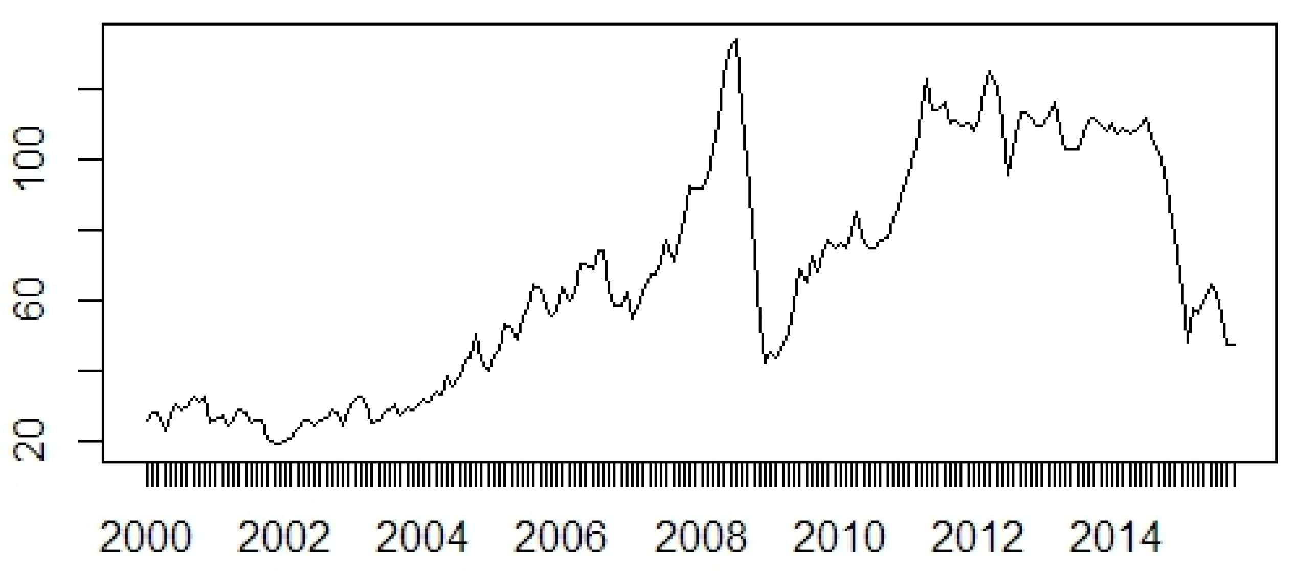
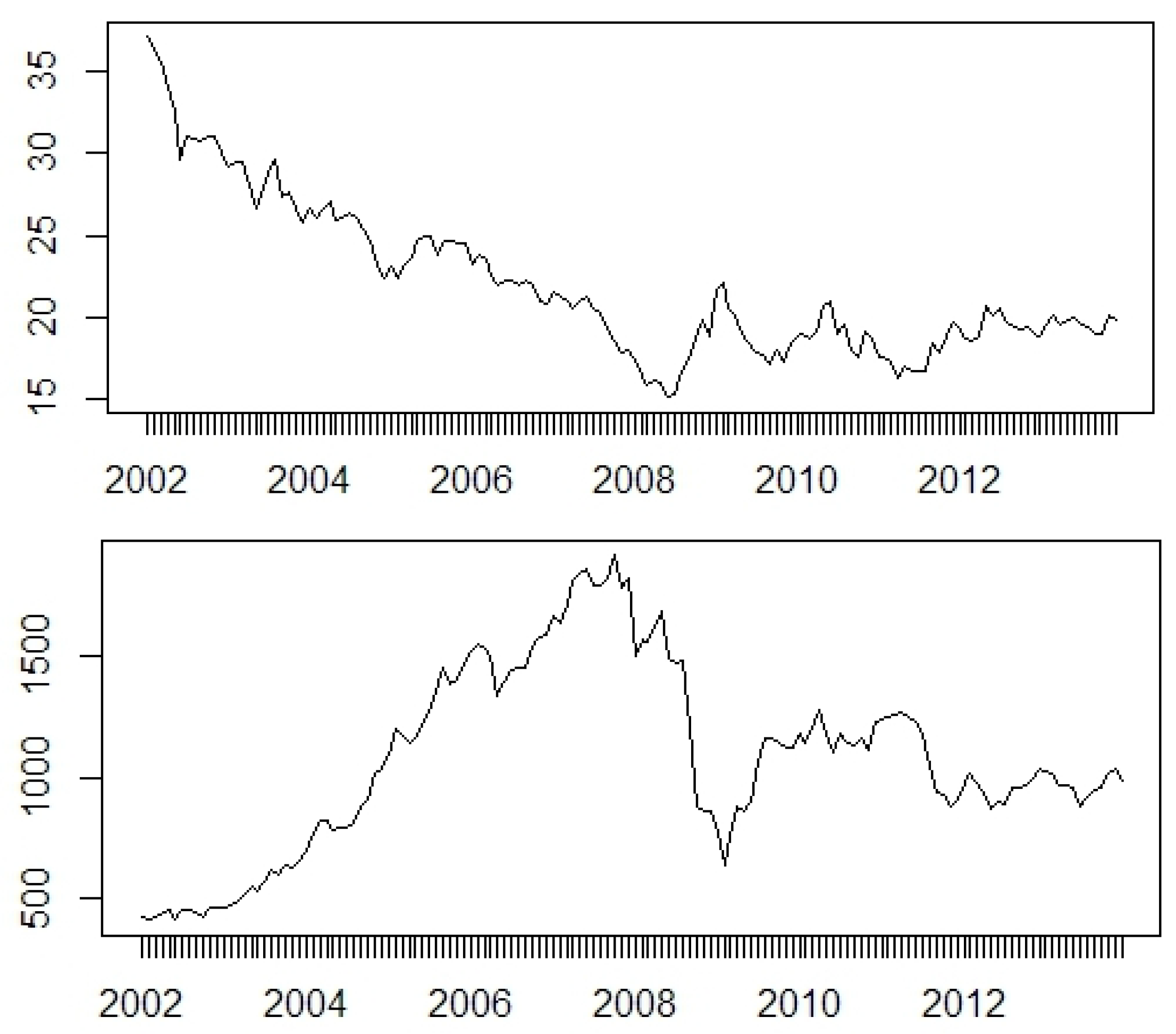
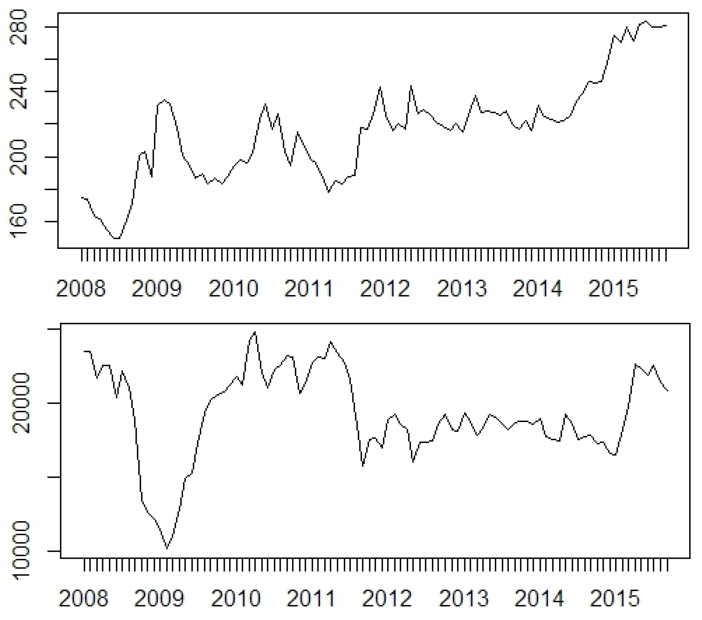
Because the CEE countries were examined, the Brent crude oil price (in USD per barrel) was taken as the oil price benchmark. Indeed, in numerous papers this price is used. This data was obtained from World Bank (2017). The aim was to focus on CEE countries, but the analysis was narrowed to Poland, the Czech Republic, Hungary, Romania, and Serbia, as out of the interesting countries for this research, these countries have a free floating exchange rate regime. The periods from which the time-series for each country were taken, were chosen with respect to this criterion. The details are presented in Table 1. The United States (US) was taken as a “benchmark” country to compare the results with. All time-series are presented in Figure 1, Figure 2, Figure 3, Figure 4, Figure 5, Figure 6 and Figure 7.
4. Methodology
The methodology was based on constructing VAR/VECMs (vector auto regression/vector error correction models) for every country with the oil price, stock market index, and exchange rate as variables (Lutkepohl 2006). The existence of a cointegrating relationship among variables was checked. Because multiple time-series were considered the Johnasen test was chosen, as it is preferred over the Engle–Granger one in such a case. This was done with the R package “urca” (Pfaff 2008a). The lag length for VAR/VECM was selected based on the Akaike Information Criterion (AIC). As monthly data were considered, up to 12 lags were tested.
The residuals from the estimated models were tested with the Breusch–Godfrey test for the lack of serial correlation, and the Jarque–Bera test of normality. Also, the ARCH-LM test was performed. The variance decomposition and impulse response among the variables is also reported in the standard way.
Additionally, Granger causality tests were performed (Granger 1969; Hothorn et al. 2017). In the past, Granger causality analysis was used in the context of oil price and USD by Nazlioglu and Soytas (2012). Of course, there exists a well-known extension of this test (Toda and Yamamoto 1995). However, this extension only usually matters if there is some uncertainty about the order of integration of variables. In this research, the standard Granger test was assumed to be enough.
To test non-linear causality the Diks–Panchenko test (DP) was used (Diks and Panchenko 2005, 2006). This test is focused on non-linear effects. As the linear ones are hoped to be captured by VAR models, it seems reasonable to perform this test to the residuals from VAR models (i.e., filter raw data by the VAR process before the test).
For the causality in variance (a spillover effect) the method by Hafner and Herwartz (2006) was used. This common test (see for example, Nazlioglu et al. (2015)) was applied for estimations from GARCH(1,1) models. According to the authors of the test, in most practical cases estimations based on such a process should be sufficient. However, a monthly frequency results in too small a sample for GARCH(1,1) estimations. Therefore, this part of the research was based on daily data (EIA 2017).
5. Results
Stationarity of all log-differenced time-series was checked. Standard tests were performed, i.e., an augmented Dickey–Fuller test (ADF), the Phillips–Perron test (PP) and the Kwiatkowski–Phillips– Schmidt–Shin (KPSS) test. The results are presented in Table 2. All calculations were done in the “tseries” R package (Trapletti et al. 2017). A detailed specification of the stationarity tests is explained in the documentation of this package. Indeed, all time-series at their first log-differences can be assumed as stationary. Generally, in all models the logarithms of the initial data were considered.
First of all, for each country it was checked whether oil price, stock market index, and exchange rate are cointegrated. The logarithms of the initial time-series can be assumed non-stationary. The results of suitable tests are in Table 3. The results of cointegration tests are reported in Table 4. Both types of the Johansen test are reported, i.e., with trace and with eigenvalue. Trend variable cointegration was assumed. The lag order of the series (levels) in the VAR was assumed to be 12, because monthly data were analyzed. The long-run specification of the VECM was assumed.
The Johansen test does not show the presence of cointegration for US and Poland. Therefore, for these countries the VAR model construction is justified. However, cointegration is found for the Czech Republic, Hungary, Romania, and Serbia. Therefore, for these countries the VECM model construction is justified. Actually, if cointegrated variables are modeled with a VAR model, then the estimations would still be consistent, but inefficient.
In Table 5, relative likelihoods derived from the Akaike information criteria (AIC) are reported for the pre-estimated VAR models with various lag length (up to 12, because monthly data were taken). The relative likelihood of the ith model is defined as:
where denotes the AIC of the model that produced the smallest AIC out of the considered 12 models. This quantity can be interpreted as how probable the given model (in comparison to the best model, i.e., the one minimizing AIC) is to minimize the information loss (Burnham and Anderson 2002). For all countries two lags are preferred due to this criterion.
Based on this, VAR/VECM models were estimated. This was done with the “var” R package (Pfaff 2008b). Technically, VECM models were transformed into level-VAR forms with respect to the already found cointegration rank. As already mentioned, for all countries two lags are strongly preferred. However, another desired feature of a VAR/VECM model is to pass the diagnostic tests. The diagnostic test results are reported in Table 6, Table 7 and Table 8. For the ultimately selected models the White test for heteroskedascity is also reported in Table 9. This test was performed with the help of the “het.test” R package (Andersson 2013).
It can be seen that fulfilling all diagnostic requirements is not always possible. As some kind of a compromise eleven lags were taken for the US and Poland, nine for the Czech Republic, six for Hungary, five for Romania, and four for Serbia.
For all of these models, moduli of the eigenvalues of the companion matrix are less than unity, which indicates the stability of the models. However, the full details are not reported. On the other hand, from Table 9, it can be seen that only the Czech Republic and Serbia have no problem with heteroskedascity.
Autocorrelation is not a desired trait, because it biases estimators and makes them less efficient. Non-normality of residuals is a minor problem. ARCH effects in residuals leads to inefficiency of estimates.
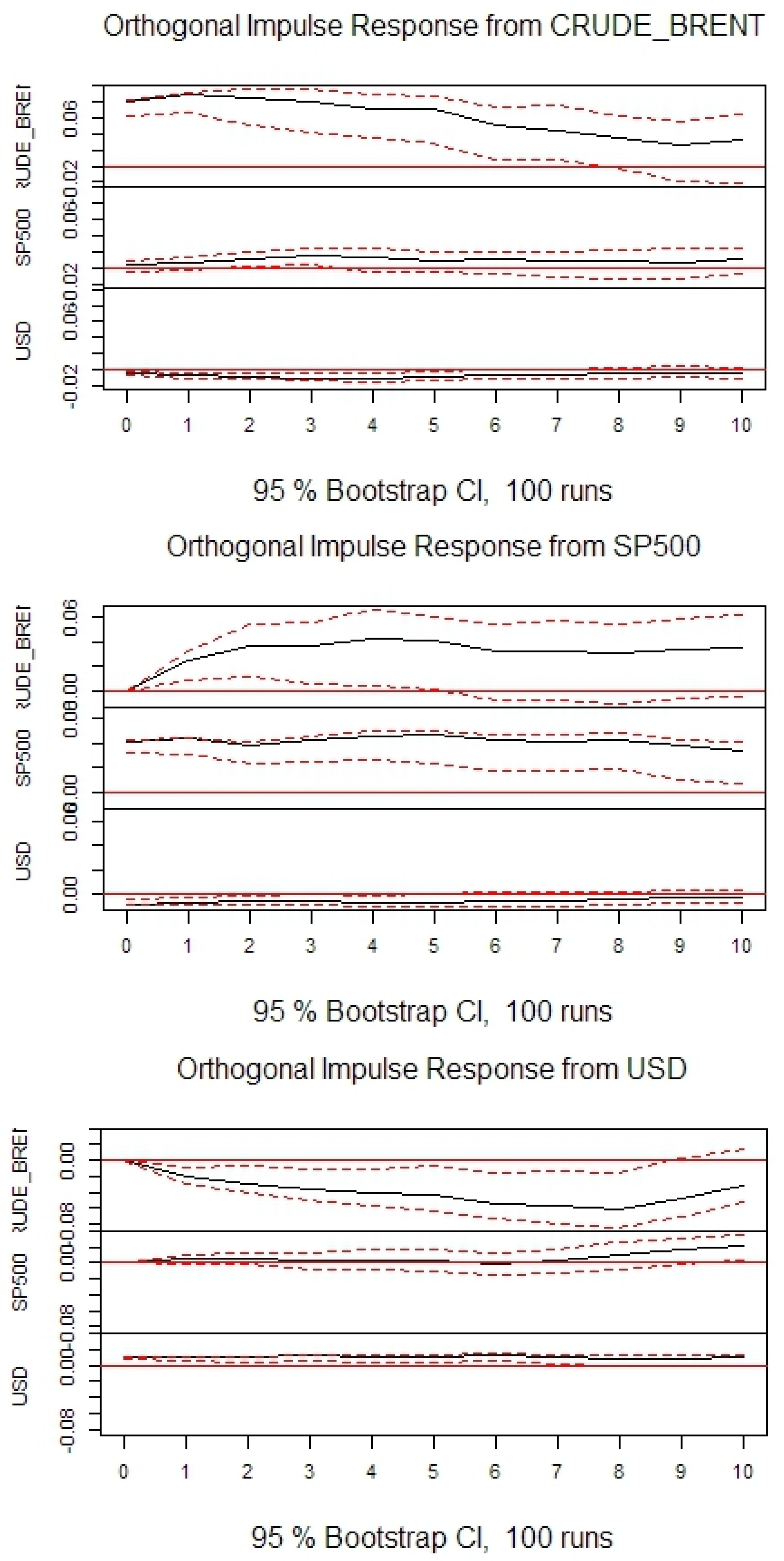
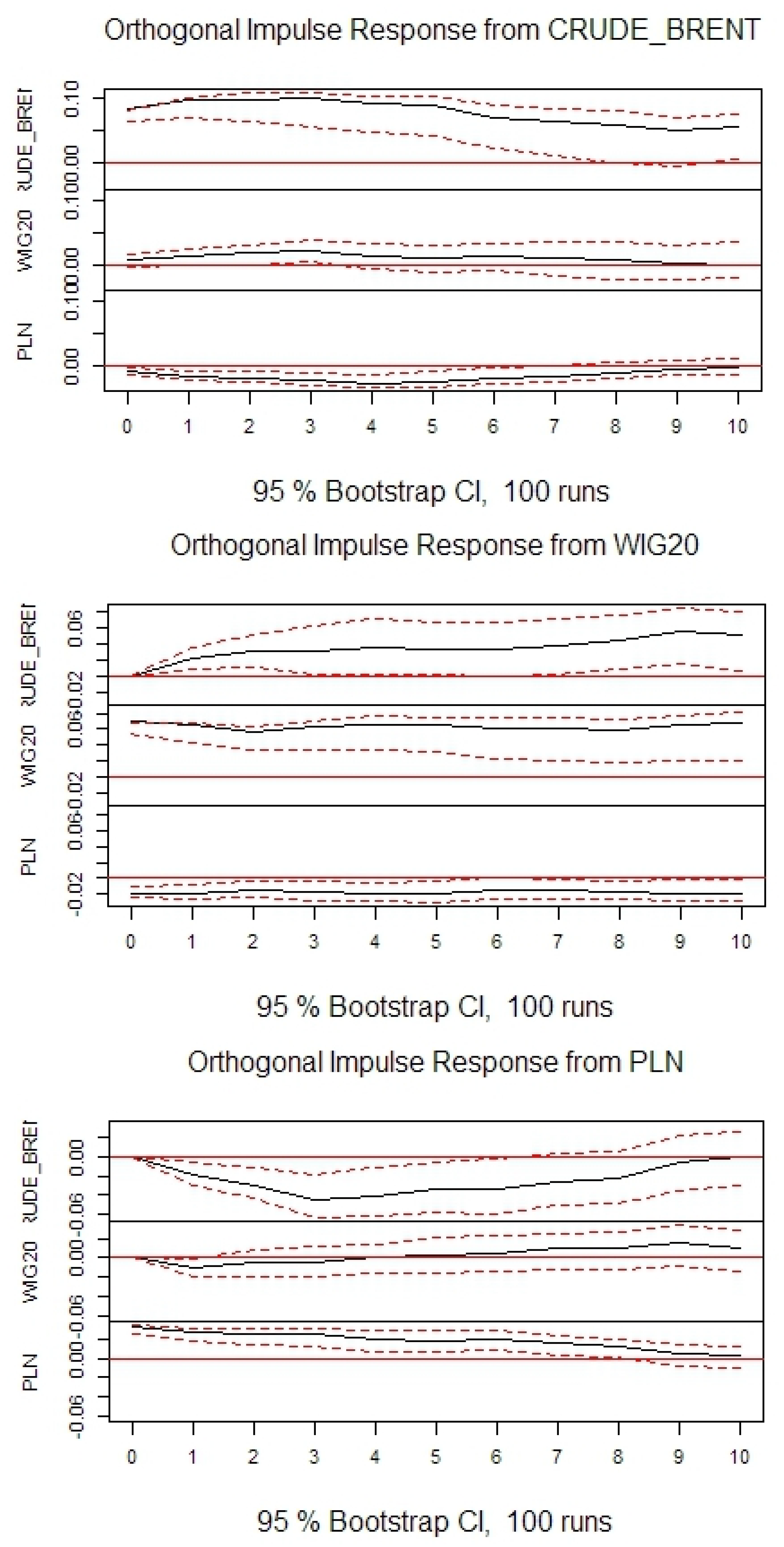
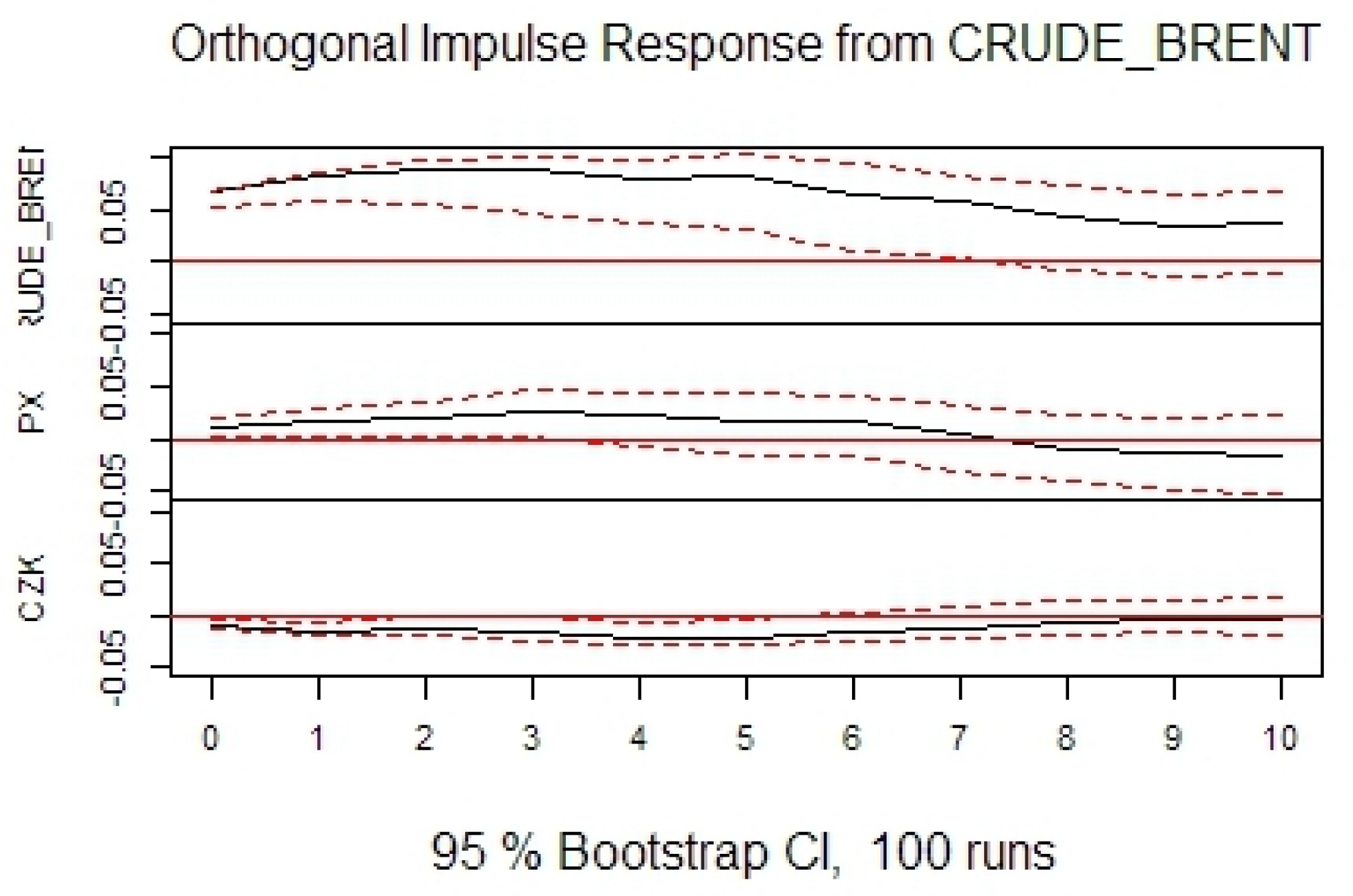
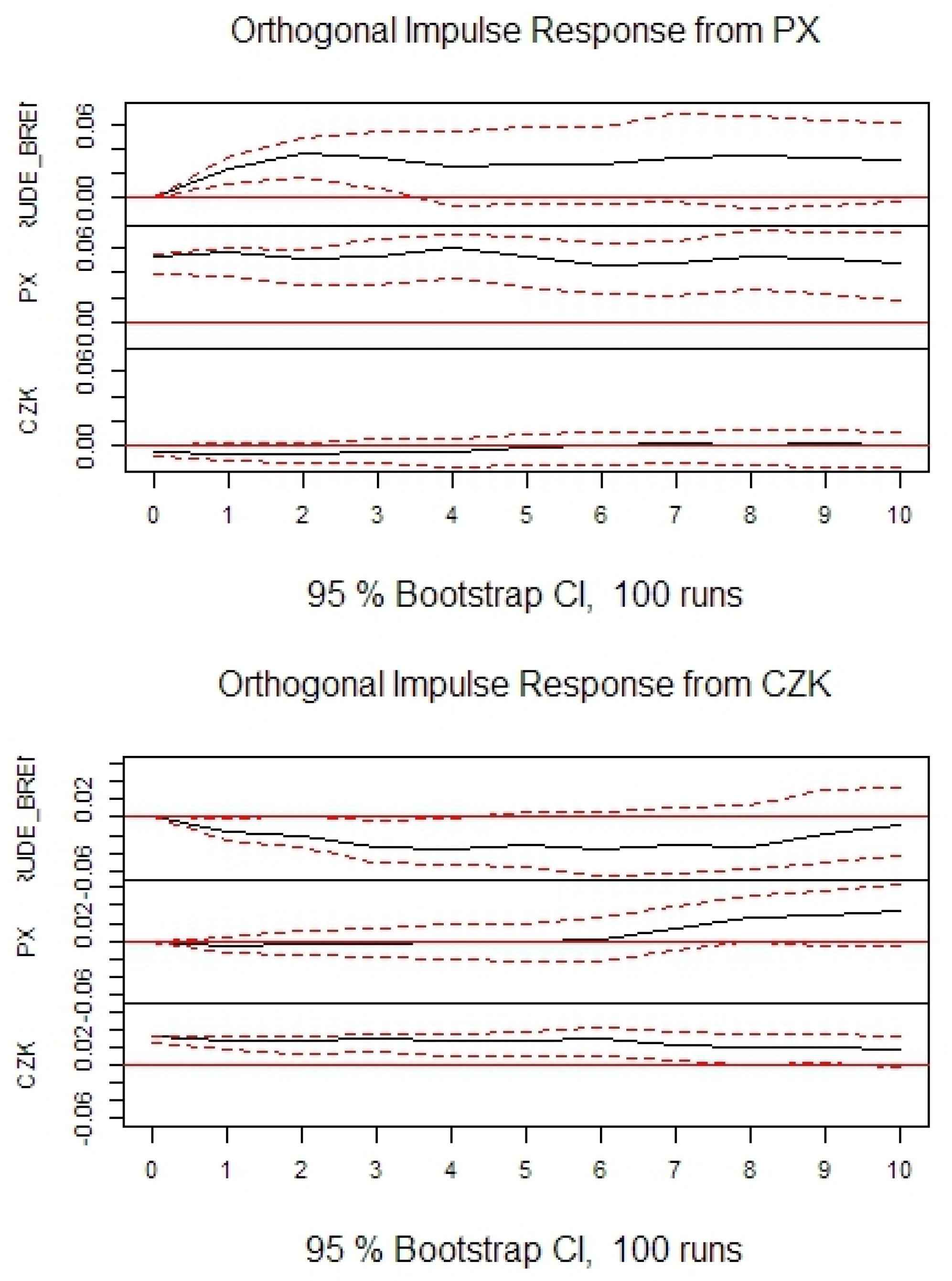
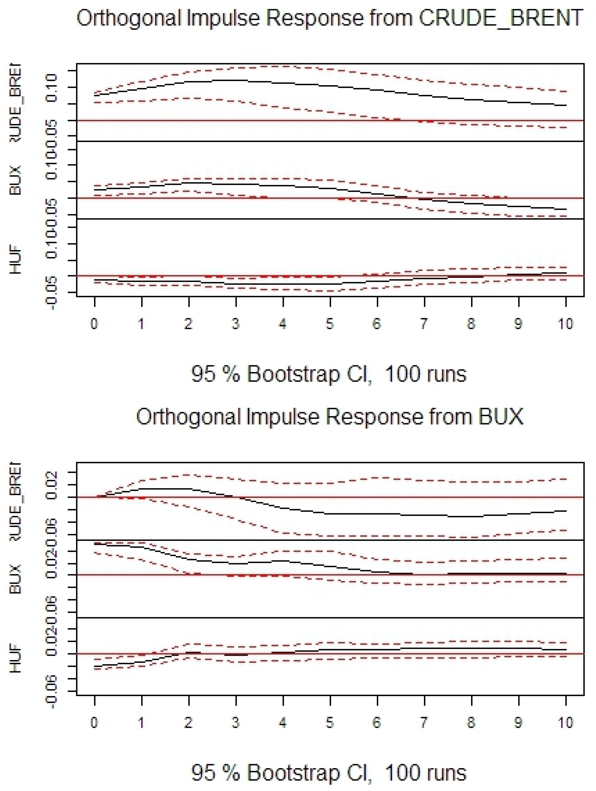
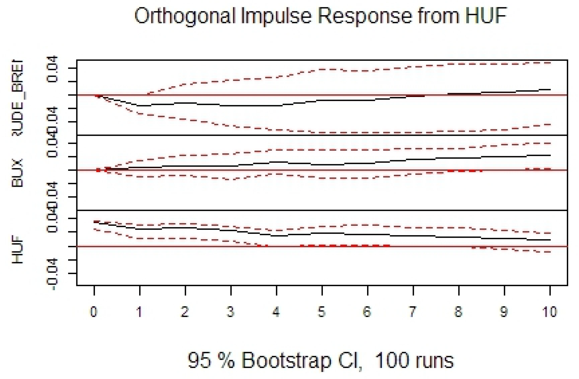
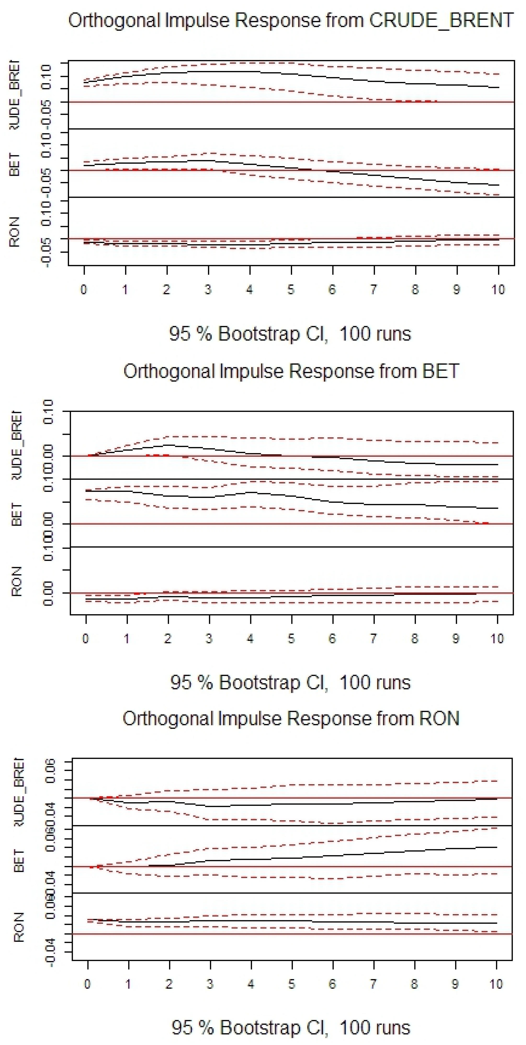
Impulse response functions are plotted in Figure 8, Figure 9, Figure 10, Figure 11, Figure 12 and Figure 13. Quantitatively, the impacts are quite small. Moreover, their signs seem to change with time.
In agreement with previous research, it can be seen that oil price negatively impacts stock prices in the long-term. However, contrary to previous research, in the short-term the effect is opposite. In agreement with previous research it can be seen that oil price negatively impacts exchange rates. It can also be seen that stock prices negatively impact exchange rates. The conclusions are generally consistent among the selected countries, as well as, when compared with the US.
The forecast error variance decomposition stabilizes very quickly. However, in Table 10 values for 12th period ahead are reported. To analyze causality in detail, the standard Granger test was performed. Its null hypothesis is that there exists no Granger causality. Outcomes are reported in Table 11. Assuming a 5% significance level for this test allows for the rejection of the null hypothesis no causality from oil price to stock prices, in the Czech Republic and Romania; from stock prices to oil price in all countries except Romania and Serbia; and from exchange rate to oil price in all countries except Romania and Serbia.
Following Bekiros and Diks (2008), the Diks–Panchenko test (DP) is reported in Table 12 and Table 13. This test was performed for both raw log-differenced data and the residuals from the above VAR models. Assuming a 5% significance level this test allows for the rejection of the null hypothesis of no causality in none of the cases. However, for filtered data this test allows for the rejection of the null hypothesis of no causality only from stock prices to oil price in Romania and from exchange rate to stock prices in Hungary.
In both tests the embedding dimension was set to the corresponding VAR/VECM lag increased by one, and the bandwidth was set to 1.5.
The results of the causality in the variance Hafner–Herwartz test are reported in Table 14. This test is based on GARCH(1,1) model, therefore, it was estimated with daily data. Monthly data did not contain enough observations to efficiently perform GARCH(1,1) estimations. Assuming a 5% significance level, this test allows for the rejection of the null hypothesis of no causality in variance from oil price to stock prices in the US, Hungary, and Romania; from oil price to exchange rate in Hungary, Romania, and Serbia; from stock prices to oil price in the US, Poland, and the Czech Republic; from stock prices to exchange rate in the US, Czech Republic, and Hungary; from exchange rate to stock prices in the US, Czech Republic, Hungary, and Romania; and from exchange rate to oil price in none of the countries.
6. Conclusions
Finally, joining all the applied methods to analyze causality (linear and non-linear), the reported methods do not bring a consistent confirmation for the existence of causalities. This conclusion has to be taken with a great caution, as there are certain problems with the diagnostic tests of the obtained VAR/VECM models.
Nevertheless, first of all it should be noted that most of the analyzed countries show similar behavior as the US (taken as a “benchmark” country here). In agreement with previous research, it was found that oil price negatively impacts stock prices—but here it was found only for the long-term. Contrary to previous research, in the short-term the effect is opposite. It was also found that oil price negatively impacts exchange rates, and that stock prices negatively impact exchange rates. The outcomes are generally consistent among the analyzed countries, and they are similar to those from the US.
The strongest linkages were found for the Czech Republic, Hungary, and Romania (both through variables and as causality in variance). Oil price impacts both stock prices and exchange rate for these countries. A weaker influence of oil price to exchange rate in Serbia was also found. However, as different tests were giving different conclusions, the outcomes should be taken with great caution.
Acknowledgments
Research was funded by a Polish National Science Centre grant, under the contract number DEC—2015/19/N/HS4/00205.
Conflicts of Interest
The author declares no conflict of interest. The founding sponsors had no role in the design of the study; in the collection, analyses, or interpretation of data; in the writing of the manuscript; and in the decision to publish the results.
References
- Abdelaziz, Mohamed, Georgios Chortareas, and Andrea Cipollini. 2008. Stock prices, exchange rates, and oil: Evidence from Middle East oil-exporting countries. Topics in Middle Eastern and African Economies 10: 1–27. [Google Scholar]
- Ahmad, Ahmad Hassan, and Ricardo Moran Hernandez. 2013. Asymmetric adjustment between oil prices and exchange rates: Empirical evidence from major oil producers and consumers. Journal of International Financial Markets Institutions & Money 27: 306–17. [Google Scholar]
- Akram, Q. Farooq. 2009. Commodity prices, interest rates and the dollar. Energy Economics 31: 838–51. [Google Scholar] [CrossRef]
- Al-mulali, Usama, Che Sab, and Che Normee Binti. 2011. The impact of oil prices on the real exchange rate of the dirham: A case study of the United Arab Emirates (UAE). OPEC Energy Review 35: 384–99. [Google Scholar] [CrossRef] [Green Version]
- Aloui, Riadh, Mohamed Safouane Ben Aïssa, and Duc Khuong Nguyen. 2013. Conditional dependence structure between oil prices and exchange rates: A copula-GARCH approach. Journal of International Money and Finance 32: 719–38. [Google Scholar] [CrossRef]
- Andersson, Sebastian. 2013. het.test: White’s Test for Heteroskedasticity. Available online: https://CRAN.R-project.org/package=het.test (accessed on 3 October 2017).
- Andrieş, Alin Marius, Iulian Ihnatov, and Aviral Kumar Tiwari. 2016. Comovement of exchange rates: A wavelet analysis. Emerging Markets Finance and Trade 52: 574–88. [Google Scholar] [CrossRef]
- Arouri, Mohamed El Hedi, Jamel Jouini, and Duc Khuong Nguyen. 2012. On the impacts of oil price fluctuations on European equity markets: Volatility spillover and hedging effectiveness. Energy Economics 34: 611–17. [Google Scholar] [CrossRef]
- Asteriou, Dimitrios, and Yuliya Bashmakova. 2013. Assessing the impact of oil returns on emerging stock markets: A panel data approach for ten Central and Eastern European Countries. Energy Economics 38: 204–11. [Google Scholar] [CrossRef]
- Bal, Debi Prasad, and Badri Narayan Rath. 2015. Nonlinear causality between crude oil price and exchange rate: A comparative study of China and India. Energy Economics 51: 149–56. [Google Scholar]
- Basher, Syed Abul, Alfred A. Haug, and Perry Sadorsky. 2012. Oil prices, exchange rates and emerging stock markets. Energy Economics 34: 227–40. [Google Scholar] [CrossRef]
- Bayat, Tayfur, Saban Nazlioglu, and Selim Kayhan. 2015. Exchange rate and oil price interactions in transition economies: Czech Republic, Hungary and Poland. Panoeconomicus 62: 267–85. [Google Scholar] [CrossRef]
- Beckmann, Joscha, and Robert Czudaj. 2013. Oil prices and effective dollar exchange rates. International Review of Economics and Finance 27: 621–36. [Google Scholar] [CrossRef]
- Beirne, John, and Martin Bijsterbosch. 2011. Exchange rate pass-through in Central and Eastern European EU member states. Journal of Policy Modeling 33: 241–54. [Google Scholar] [CrossRef]
- Bekiros, Stelios D., and Cees GH Diks. 2008. The relationship between crude oil spot and futures prices: Cointegration, linear and nonlinear causality. Energy Economics 30: 2673–85. [Google Scholar] [CrossRef]
- Belke, Ansgar, and Albina Zenkic. 2007. Exchange-rate regimes and the transition process in the Western Balkans: A comparative analysis. Intereconomics 42: 267–80. [Google Scholar] [CrossRef] [Green Version]
- Bodart, Vincent, Bertrand Candelon, and Jean-François Carpantier. 2015. Real exchanges rates, commodity prices and structural factors in developing countries. Journal of International Money and Finance 51: 264–84. [Google Scholar] [CrossRef]
- Brahmasrene, Tantatape, Jui-Chi Huang, and Yaya Sissoko. 2014. Crude oil prices and exchange rates: Causality, variance decomposition and impulse response. Energy Economics 44: 407–12. [Google Scholar] [CrossRef]
- Broda, Christian. 2004. Terms of trade and exchange rate regimes in developing countries. Journal of International Economics 63: 31–58. [Google Scholar] [CrossRef]
- BSE. 2016. Historical Data. Available online: http://www.belex.rs/eng/trgovanje/indeksi/belex15 (accessed on 3 October 2017).
- Burnham, Kenneth P., and David R. Anderson. 2002. Model Selection and Multimodel Inference: A Practical Information-Theoretic Approach. New York: Springer. [Google Scholar]
- Causevic, Fikret. 2015. Globalization, Southeastern Europe, and the World Economy. Oxon: Routledge. [Google Scholar]
- Ciner, Cetin, Constantin Gurdgiev, and Brian M. Lucey. 2013. Hedges and safe havens: An examination of stocks, bonds, gold, oil and exchange rates. International Review of Financial Analysis 29: 202–11. [Google Scholar] [CrossRef]
- Diks, Cees, and Valentyn Panchenko. 2005. A note on the Hiemstra-Jones test for Granger non-causality. Studies in Nonlinear Dynamics & Econometrics 9. [Google Scholar] [CrossRef]
- Diks, Cees, and Valentyn Panchenko. 2006. A new statistic and practical guidelines for nonparametric Granger causality testing. Journal of Economic Dynamics & Control 30: 1647–69. [Google Scholar]
- Ding, Liang, and Minh Vo. 2012. Exchange rates and oil prices: A multivariate stochastic volatility analysis. The Quarterly Review of Economics and Finance 52: 15–37. [Google Scholar] [CrossRef]
- U.S. Energy Information Administration (EIA). 2015. International Energy Statistics; Technical Report. Washington: U.S. Energy Information Administration.
- U.S. Energy Information Administration (EIA). 2017. Petroleum & Other Liquids. Available online: https://www.eia.gov/dnav/pet/PETPRISPTS1D.htm (accessed on 3 October 2017).
- Ferraro, Domenico, Kenneth Rogoff, and Barbara Rossi. 2015. Can oil prices forecast exchange rates? An empirical analysis of the relationship between commodity prices and exchange rates. Journal of International Money and Finance 54: 116–41. [Google Scholar] [CrossRef]
- FRED. 2016. Trade Weighted U.S. Dollar Index: Broad. Available online: https://fred.stlouisfed.org/series/DTWEXB (accessed on 3 October 2017).
- Ghosh, Sajal. 2011. Examining crude oil price—Exchange rate nexus for India during the period of extreme oil price volatility. Applied Energy 88: 1886–89. [Google Scholar] [CrossRef]
- Golub, Stephen S. 1983. Oil price and exchange rates. The Economic Journal 93: 576–93. [Google Scholar] [CrossRef]
- Granger, Clive WJ. 1969. Investigating causal relations by econometric models and cross-spectral methods. Econometrica 37: 424–38. [Google Scholar] [CrossRef]
- Habib, Maurizio Michael, and Margarita M. Kalamova. 2007. Are There Oil Currencies? The Real Exchange Rate of Oil-Exporting Countries. Technical Report. Frankfurt am Main: European Central Bank. [Google Scholar]
- Hafner, Christian M., and Helmut Herwartz. 2006. A Lagrange multiplier test for causality in variance. Economics Letters 93: 137–41. [Google Scholar] [CrossRef]
- Hamilton, James D. 2003. What is an oil shock? Journal of Econometrics 113: 363–98. [Google Scholar] [CrossRef]
- Fakhri, Hasanov. 2010. The Impact of Real Oil Price on Real Effective Exchange Rate: The Case of Azerbaijan. Technical Report. Berlin: DIW Berlin. [Google Scholar]
- Fakhri, Hasanov, Jeyhun Mikayilov, Cihan Bulut, Elchin Suleymanov, and Dr Aliyev. 2017. The role of oil prices in exchange rate movements: The CIS oil exporters. Economies 5: 13. [Google Scholar]
- Hothorn, Torsten, Achim Zeileis, Richard W. Farebrother, Clint Cummins, Giovanni Millo, and David Mitchell. 2017. Testing Linear Regression Models. Available online: https://cran.r-project.org/package=lmtest (accessed on 3 October 2017).
- Huang, Alexi Y., and Yi-Heng Tseng. 2010. Is crude oil price affected by the US dollar exchange rate? International Research Journal of Finance and Economics 58: 109–20. [Google Scholar]
- Ilzetzki, Ethan, Carmen M. Reinhart, and Kenneth S. Rogoff. 2017. Exchange Rate Arrangements Entering The 21st Century: Which Anchor Will Hold? NBER Working Paper 23134. Cambridge, MA, USA: National Bureau of Economic Research. [Google Scholar]
- International Monetary Fund (IMF). 2009. Annual Report on Exchange Arrangements and Exchange Restrictions. Technical Report. Washington: International Monetary Fund. [Google Scholar]
- International Monetary Fund (IMF). 2015. Central and Eastern Europe: New Member States (NMS) Policy Forum. Technical Report. Washington: International Monetary Fund. [Google Scholar]
- INVESTING.COM. 2016. USD/RSD—US Dollar Serbian Dinar. Available online: https://www.investing.com/currencies/usd-rsd-historical-data (accessed on 3 October 2017).
- Josifidis, Kosta, Jean-Pierre Allegret, and Emilija Beker Pucar. 2009. Monetary and exchange rate regime changes: The case of Poland, Czech Republic, Slovakia and Republic of Serbia. Panoeconomicus 56: 199–226. [Google Scholar] [CrossRef]
- Kalcheva, Katerina, and Nienke Oomes. 2007. Diagnosing Dutch Disease: Does Russia Have the Symptoms? Technical Report. Washington: International Monetary Fund. [Google Scholar]
- Kilian, Lutz. 2006. Not all oil price shocks are alike: Disentangling demand and supply shocks in the crude oil market. American Economic Review 99: 1053–69. [Google Scholar] [CrossRef]
- Lutkepohl, Helmut. 2006. New Introduction to Multiple Time Series Analysis. Berlin: Springer. [Google Scholar]
- Mihaljek, Dubravko. 2009. The financial stability implications of increased capital flows for emerging market economies. BIS Papers 44: 11–44. [Google Scholar]
- Mirdala, Rajmund. 2013. Current account adjustments and real exchange rates in European transition economies. Journal of Applied Economic Sciences 2: 210–27. [Google Scholar]
- Mohammadi, Hassan, and Mohammad R. Jahan-Parvar. 2010. Oil prices and exchange rates in oil-exporting countries: Evidence from TAR and M-TAR models. Journal of Economics and Finance 36: 1–14. [Google Scholar] [CrossRef]
- Mucuk, Mehmet, and Ibrahim Halil Sugozu. 2011. Sectoral energy consumption and economic growth nexus in Turkey. Energy Education Science and Technology Part B Social and Educational Studies 3: 441–48. [Google Scholar]
- Narayan, Seema. 2013. Foreign exchange markets and oil prices in Asia. Journal of Asian Economics 28: 41–50. [Google Scholar] [CrossRef]
- Nazlioglu, Saban, and Ugur Soytas. 2012. Oil price, agricultural commodity prices, and the dollar: A panel cointegration and causality analysis. Energy Economics 34: 1098–1104. [Google Scholar] [CrossRef]
- Nazlioglu, Saban, Ugur Soytas, and Rangan Gupta. 2015. Oil prices and financial stress: A volatility spillover analysis. Energy Policy 82: 278–88. [Google Scholar] [CrossRef]
- Novotný, Filip. 2012. The link between the Brent crude oil price and the US dollar exchange rate. Prague Economic Papers 21: 220–32. [Google Scholar] [CrossRef]
- Pfaff, Bernhard. 2008a. Analysis of Integrated and Cointegrated Time Series with R. Berlin: Springer. [Google Scholar]
- Pfaff, Bernhard. 2008b. VAR, SVAR and SVEC Models: Implementation within R package vars. Journal of Statistical Software 27: 1–32. [Google Scholar] [CrossRef]
- Popescu, Gheorghe H. 2014. FDI and economic growth in Central and Eastern Europe. Sustainability 6: 8149–63. [Google Scholar] [CrossRef]
- Reboredo, Juan C. 2012. Modelling oil price and exchange rate co-movements. Journal of Policy Modeling 34: 419–40. [Google Scholar] [CrossRef]
- Reboredo, Juan C., and Miguel A. Rivera-Castro. 2013. A wavelet decomposition approach to crude oil price and exchange rate dependence. Economic Modelling 32: 42–57. [Google Scholar] [CrossRef]
- Ryan, Jeffrey A., and Joshua M. Ulrich. 2017. xts: eXtensible Time Series. Available online: https://CRAN.R-project.org/package=xts (accessed on 3 October 2017).
- Scholtens, Bert, and Cenk Yurtsever. 2012. Oil price shocks and European industries. Energy Economics 34: 1187–95. [Google Scholar] [CrossRef]
- STOOQ. 2016. Quotes. Available online: https://stooq.com (accessed on 3 October 2017).
- Tiwari, Aviral Kumar, Mihai Ioan Mutascu, and Claudiu Tiberiu Albulescu. 2013. The influence of the international oil prices on the real effective exchange rate in Romania in a wavelet transform framework. Energy Economics 40: 714–33. [Google Scholar] [CrossRef]
- Toda, Hiro Y., and Taku Yamamoto. 1995. Statistical inference in Vector Autoregressions with possibly integrated processes. Journal of Econometrics 66: 225–50. [Google Scholar] [CrossRef]
- Trapletti, Adrian, Kurt Hornik, and Blake LeBaron. 2017. Time Series Analysis and Computational Finance. Available online: https://cran.r-project.org/package=tseries (accessed on 3 October 2017).
- Turhan, Ibrahim, Erk Hacihasanoglu, and Ugur Soytas. 2013. Oil prices and emerging market exchange rates. Emerging Markets Finance and Trade 49: 21–36. [Google Scholar] [CrossRef]
- Uddin, Gazi Salah, Aviral Kumar Tiwari, Mohamed Arouri, and Frederic Teulon. 2013. On the relationship between oil price and exchange rates: A wavelet analysis. Economic Modelling 35: 502–7. [Google Scholar] [CrossRef]
- World Bank. 2015. World Bank Open Data. Technical Report. Washington: The World Bank. [Google Scholar]
- World Bank. 2017. Global Economic Monitor Commodities. Washington: The World Bank, Available online: http://databank.worldbank.org/data/reports.aspx?source=global-economic-monitor-commodities (accessed on 3 October 2017).
- Wu, Chih-Chiang, Huimin Chung, and Yu-Hsien Chang. 2012. The economic value of co-movement between oil price and exchange rate using copula-based GARCH models. Energy Economics 34: 270–82. [Google Scholar] [CrossRef]
- Zhang, Yue-Jun, Ying Fan, Hsien-Tang Tsai, and Yi-Ming Wei. 2008. Spillover effect of US dollar exchange rate on oil prices. Journal of Policy Modeling 30: 973–91. [Google Scholar] [CrossRef]
Figure 1.
Brent oil price.

Figure 2.
Exchange rate (top) and stock index (bottom) for the US.

Figure 3.
Exchange rate (top) and stock index (bottom) for Poland.

Figure 4.
Exchange rate (top) and stock index (bottom) for the Czech Republic.

Figure 5.
Exchange rate (top) and stock index (bottom) for Hungary.

Figure 6.
Exchange rate (top) and stock index (bottom) for Romania.

Figure 7.
Exchange rate (top) and stock index (bottom) for Serbia.

Figure 8.
Impulse response for the US.

Figure 9.
Impulse response for Poland.

Figure 10.
Impulse response for the Czech Republic.


Figure 11.
Impulse response for Hungary.


Figure 12.
Impulse response for Romania.

Figure 13.
Impulse response for Serbia.


Table 1.
Data abbreviations and details.
| Abbreviation | Description | Time Period | No of Obs. | Source |
|---|---|---|---|---|
| SP500 | US stock market index | January 2000/September 2015 | 189 | STOOQ (2016) |
| WIG20 | Polish stock market index | January 2000/September 2015 | 189 | STOOQ (2016) |
| PX | Czech stock market index | January 2002/December 2013 | 144 | STOOQ (2016) |
| BUX | Hungarian stock market index | January 2008/September 2015 | 93 | STOOQ (2016) |
| BET | Romanian stock market index | January 2005/September 2015 | 129 | STOOQ (2016) |
| BELEX | Serbian stock market index | January 2009/September 2015 | 81 | BSE (2016) |
| USD | Trade weighted US dollar index | January 2000/September 2015 | 189 | FRED (2016) |
| PLN | US dollar/Polish zloty | January 2000/September 2015 | 189 | STOOQ (2016) |
| CZK | US dollar/Czech koruna | January 2002/December 2013 | 144 | STOOQ (2016) |
| HUF | US dollar/Hungarian forint | January 2008/September 2015 | 93 | STOOQ (2016) |
| RON | US dollar/Romanian leu | January 2005/September 2015 | 129 | STOOQ (2016) |
| RSD | US dollar/Serbian dinar | January 2009/September 2015 | 81 | INVESTING.COM (2016) |
Table 2.
Stationarity tests for first log-differences of time-series.
| Variable | ADF Stat. | ADF p-Value | KPSS Stat. | KPSS p-Value | PP Stat. | PP p-Value |
|---|---|---|---|---|---|---|
| BRENT | −6.4489 | 0.0100 | 0.2013 | 0.1000 | −151.6985 | 0.0100 |
| SP500 | −5.2475 | 0.0100 | 0.2152 | 0.1000 | −171.1551 | 0.0100 |
| WIG20 | −4.7473 | 0.0100 | 0.1014 | 0.1000 | −193.1045 | 0.0100 |
| PX | −5.0212 | 0.0100 | 0.4243 | 0.0667 | −122.0051 | 0.0100 |
| BUX | −4.0322 | 0.0113 | 0.0845 | 0.1000 | −66.9895 | 0.0100 |
| BET | −4.1660 | 0.0100 | 0.0786 | 0.1000 | −109.7117 | 0.0100 |
| BELEX | −4.1385 | 0.0100 | 0.0540 | 0.1000 | −54.8673 | 0.0100 |
| USD | −4.7591 | 0.0100 | 0.2971 | 0.1000 | −187.9259 | 0.0100 |
| PLN | −5.5965 | 0.0100 | 0.1582 | 0.1000 | −179.9251 | 0.0100 |
| CZK | −4.7942 | 0.0100 | 0.3051 | 0.1000 | −147.1142 | 0.0100 |
| HUF | −4.5151 | 0.0100 | 0.0372 | 0.1000 | −98.0126 | 0.0100 |
| RON | −4.3504 | 0.0100 | 0.1074 | 0.1000 | −139.7213 | 0.0100 |
| RSD | −3.4359 | 0.0557 | 0.0999 | 0.1000 | −90.7951 | 0.0100 |
Table 3.
Stationarity tests for logarithms of time-series.
| Variable | ADF Stat. | ADF p-Value | KPSS Stat. | KPSS p-Value | PP Stat. | PP p-Value |
|---|---|---|---|---|---|---|
| BRENT | −1.4501 | 0.8062 | 3.7208 | 0.0100 | −6.4696 | 0.7449 |
| SP500 | −2.7133 | 0.2778 | 1.8264 | 0.0100 | −7.4644 | 0.6882 |
| WIG20 | −2.1702 | 0.5050 | 1.9076 | 0.0100 | −7.0990 | 0.7090 |
| PX | −2.1256 | 0.5241 | 1.4797 | 0.0100 | −4.2770 | 0.8693 |
| BUX | −3.7373 | 0.0253 | 0.1299 | 0.1000 | −12.8294 | 0.3671 |
| BET | −2.5452 | 0.3499 | 0.4746 | 0.0474 | −8.5555 | 0.6220 |
| BELEX | −2.8378 | 0.2327 | 0.2714 | 0.1000 | −10.3543 | 0.5071 |
| USD | −0.6197 | 0.9755 | 2.9930 | 0.0100 | −1.7697 | 0.9747 |
| PLN | −1.9390 | 0.6017 | 2.0081 | 0.0100 | −7.8566 | 0.6659 |
| CZK | −1.7658 | 0.6739 | 3.6240 | 0.0100 | −10.1741 | 0.5299 |
| HUF | −3.8525 | 0.0197 | 2.1087 | 0.0100 | −20.5839 | 0.0498 |
| RON | −3.1003 | 0.1191 | 2.8040 | 0.0100 | −12.9520 | 0.3681 |
| RSD | −3.4319 | 0.0562 | 2.0115 | 0.0100 | −13.0083 | 0.3497 |
Table 4.
Results of the Johansen cointegration test.
| Stat. for Trace Test | 5% cr. Val. for Trace Test | Stat. for Eigenvalue Test | 5% cr. Val. for Eigenvalue Test | |
|---|---|---|---|---|
| US | ||||
| r ≤ 2 | 5.9702 | 12.2500 | 5.9702 | 12.2500 |
| r ≤ 1 | 17.5022 | 25.3200 | 11.5320 | 18.9600 |
| r = 0 | 36.7542 | 42.4400 | 19.2520 | 25.5400 |
| Poland | ||||
| r ≤ 2 | 3.6402 | 12.2500 | 3.6402 | 12.2500 |
| r ≤ 1 | 10.4185 | 25.3200 | 6.7783 | 18.9600 |
| r = 0 | 40.3358 | 42.4400 | 29.9172 | 25.5400 |
| Czech Republic | ||||
| r ≤ 2 | 6.6863 | 12.2500 | 6.6863 | 12.2500 |
| r ≤ 1 | 21.4958 | 25.3200 | 14.8095 | 18.9600 |
| r = 0 | 56.1004 | 42.4400 | 34.6047 | 25.5400 |
| Hungary | ||||
| r ≤ 2 | 11.0812 | 12.2500 | 11.0812 | 12.2500 |
| r ≤ 1 | 32.5795 | 25.3200 | 21.4983 | 18.9600 |
| r = 0 | 67.7358 | 42.4400 | 35.1562 | 25.5400 |
| Romania | ||||
| r ≤ 2 | 4.7307 | 12.2500 | 4.7307 | 12.2500 |
| r ≤ 1 | 24.3996 | 25.3200 | 19.6689 | 18.9600 |
| r = 0 | 60.9070 | 42.4400 | 36.5074 | 25.5400 |
| Serbia | ||||
| r ≤ 2 | 8.7501 | 12.2500 | 8.7501 | 12.2500 |
| r ≤ 1 | 21.9862 | 25.3200 | 13.2360 | 18.9600 |
| r = 0 | 62.3504 | 42.4400 | 40.3642 | 25.5400 |
Table 5.
Relative likelihoods for vector auto regression (VAR) (p)-processes.
| p | US | Poland | Czech Republic | Hungary | Romania | Serbia |
|---|---|---|---|---|---|---|
| 1 | 0.9708 | 0.9627 | 0.9395 | 0.9596 | 0.8887 | 0.9772 |
| 2 | 1.0000 | 1.0000 | 1.0000 | 1.0000 | 1.0000 | 1.0000 |
| 3 | 0.9721 | 0.9755 | 0.9806 | 0.9859 | 0.9973 | 0.9411 |
| 4 | 0.9497 | 0.9589 | 0.9506 | 0.9396 | 0.9680 | 0.8817 |
| 5 | 0.9432 | 0.9707 | 0.9364 | 0.9928 | 0.9519 | 0.9065 |
| 6 | 0.9228 | 0.9401 | 0.9196 | 0.9344 | 0.9193 | 0.8257 |
| 7 | 0.9192 | 0.9449 | 0.9151 | 0.8942 | 0.8742 | 0.8354 |
| 8 | 0.9172 | 0.9172 | 0.9093 | 0.8342 | 0.8324 | 0.7557 |
| 9 | 0.9029 | 0.8846 | 0.8928 | 0.8032 | 0.7881 | 0.7262 |
| 10 | 0.8914 | 0.8907 | 0.8638 | 0.8138 | 0.7820 | 0.7840 |
| 11 | 0.8839 | 0.8734 | 0.8624 | 0.7706 | 0.8021 | 0.8169 |
| 12 | 0.8518 | 0.8587 | 0.8670 | 0.7466 | 0.8617 | 0.8208 |
Table 6.
Diagnostic tests (p-values) for the Breusch–Godfrey test.
| Lags | US | Poland | Czech Republic | Hungary | Romania | Serbia |
|---|---|---|---|---|---|---|
| 1 | 0.0185 | 0.0117 | 0.3755 | 0.0469 | 0.4217 | 0.4752 |
| 2 | 0.5211 | 0.2830 | 0.2454 | 0.0156 | 0.0603 | 0.3710 |
| 3 | 0.0594 | 0.0017 | 0.2011 | 0.2783 | 0.1684 | 0.0427 |
| 4 | 0.0965 | 0.0305 | 0.0021 | 0.0362 | 0.4261 | 0.0424 |
| 5 | 0.1368 | 0.5433 | 0.0098 | 0.0444 | 0.5959 | 0.0096 |
| 6 | 0.0326 | 0.4269 | 0.0238 | 0.0102 | 0.3551 | 0.0002 |
| 7 | 0.0174 | 0.0083 | 0.1297 | 0.0007 | 0.0044 | 0.0096 |
| 8 | 0.0259 | 0.0014 | 0.1249 | 0.0000 | 0.0002 | 0.0021 |
| 9 | 0.0063 | 0.0190 | 0.0098 | 0.0000 | 0.0003 | 0.0000 |
| 10 | 0.0100 | 0.0780 | 0.0088 | 0.0000 | 0.0000 | 0.0000 |
| 11 | 0.0021 | 0.0378 | 0.0074 | 0.0000 | 0.0000 | 0.0000 |
| 12 | 0.0218 | 0.0778 | 0.0031 | 0.0000 | 0.0000 | 0.0000 |
Table 7.
Diagnostic tests (p-values) for the Jarque–Bera test.
| Lags | US | Poland | Czech Republic | Hungary | Romania | Serbia |
|---|---|---|---|---|---|---|
| 1 | 0.0000 | 0.0000 | 0.0000 | 0.0002 | 0.0000 | 0.0037 |
| 2 | 0.0000 | 0.0000 | 0.0000 | 0.0002 | 0.0000 | 0.0037 |
| 3 | 0.0000 | 0.0000 | 0.0000 | 0.0030 | 0.0005 | 0.0051 |
| 4 | 0.0000 | 0.0002 | 0.0000 | 0.0071 | 0.0023 | 0.0142 |
| 5 | 0.0001 | 0.0007 | 0.0087 | 0.0726 | 0.0232 | 0.0001 |
| 6 | 0.0007 | 0.0003 | 0.0001 | 0.0476 | 0.2583 | 0.0001 |
| 7 | 0.0031 | 0.0011 | 0.0001 | 0.0233 | 0.3031 | 0.0000 |
| 8 | 0.0079 | 0.0013 | 0.0000 | 0.0000 | 0.2307 | 0.0000 |
| 9 | 0.0045 | 0.0054 | 0.0000 | 0.0000 | 0.1990 | 0.0000 |
| 10 | 0.0022 | 0.0068 | 0.0000 | 0.0451 | 0.0993 | 0.0000 |
| 11 | 0.0105 | 0.0130 | 0.0000 | 0.0092 | 0.1811 | 0.0000 |
| 12 | 0.0051 | 0.0140 | 0.0000 | 0.0000 | 0.0002 | 0.0155 |
Table 8.
Diagnostic tests (p-values) for the ARCH-LM test.
| Lags | US | Poland | Czech Republic | Hungary | Romania | Serbia |
|---|---|---|---|---|---|---|
| 1 | 0.0000 | 0.0000 | 0.0002 | 0.0000 | 0.0000 | 0.0245 |
| 2 | 0.0000 | 0.0822 | 0.0000 | 0.0000 | 0.0000 | 0.0428 |
| 3 | 0.0000 | 0.0071 | 0.0049 | 0.0002 | 0.0001 | 0.0052 |
| 4 | 0.0000 | 0.0444 | 0.0003 | 0.0038 | 0.0007 | 0.0711 |
| 5 | 0.0004 | 0.0509 | 0.0007 | 0.0244 | 0.0010 | 0.0034 |
| 6 | 0.0059 | 0.1500 | 0.0028 | 0.0568 | 0.0004 | 0.0037 |
| 7 | 0.0024 | 0.0698 | 0.0023 | 0.3340 | 0.0011 | 0.2907 |
| 8 | 0.0245 | 0.0949 | 0.0092 | 0.3238 | 0.0031 | 0.3151 |
| 9 | 0.2362 | 0.0834 | 0.0131 | 0.2398 | 0.0212 | 0.2645 |
| 10 | 0.2375 | 0.0979 | 0.0539 | 0.4578 | 0.0149 | 0.4024 |
| 11 | 0.2466 | 0.2578 | 0.1906 | 0.4801 | 0.0708 | 0.9363 |
| 12 | 0.2350 | 0.1539 | 0.0812 | 0.7252 | 0.2039 | 0.9995 |
Table 9.
White test (p-values) for heteroscedasticity (for the final models).
| US | Poland | Czech Republic | Hungary | Romania | Serbia |
|---|---|---|---|---|---|
| 0.0057 | 0.0085 | 0.1178 | 0.0000 | 0.0000 | 0.1066 |
Table 10.
Forecast error variance decomposition.
| Oil Price | Stock Prices | Exchange Rate | |
|---|---|---|---|
| US | |||
| BRENT | 0.5841 | 0.1588 | 0.2571 |
| SP500 | 0.0508 | 0.8824 | 0.0668 |
| USD | 0.2244 | 0.1646 | 0.6110 |
| Poland | |||
| BRENT | 0.7350 | 0.1813 | 0.0837 |
| WIG20 | 0.0276 | 0.9558 | 0.0166 |
| PLN | 0.3061 | 0.3245 | 0.3694 |
| Czech Republic | |||
| BRENT | 0.7472 | 0.1420 | 0.1108 |
| PX | 0.0846 | 0.8039 | 0.1115 |
| CZK | 0.2039 | 0.0188 | 0.7772 |
| Hungary | |||
| BRENT | 0.9354 | 0.0524 | 0.0123 |
| BUX | 0.5628 | 0.3180 | 0.1192 |
| HUF | 0.3594 | 0.1031 | 0.5374 |
| Romania | |||
| BRENT | 0.9639 | 0.0248 | 0.0113 |
| BET | 0.2570 | 0.6115 | 0.1315 |
| RON | 0.2087 | 0.0840 | 0.7073 |
| Serbia | |||
| BRENT | 0.8157 | 0.1022 | 0.0821 |
| BELEX | 0.0968 | 0.7248 | 0.1784 |
| RSD | 0.0797 | 0.0418 | 0.8785 |
Table 11.
Granger test (p-values).
| US | Poland | Czech Republic | Hungary | Romania | Serbia | |
|---|---|---|---|---|---|---|
| oil price → stock prices | 0.4916 | 0.7668 | 0.0366 | 0.5388 | 0.0010 | 0.2937 |
| oil price → exchange rate | 0.3139 | 0.2429 | 0.2981 | 0.1851 | 0.3214 | 0.6877 |
| stock prices → oil price | 0.0169 | 0.0288 | 0.0051 | 0.0452 | 0.2869 | 0.2113 |
| stock prices → exchange rate | 0.4636 | 0.2614 | 0.1364 | 0.0597 | 0.2710 | 0.2823 |
| exchange rate → stock prices | 0.8973 | 0.1089 | 0.2541 | 0.6893 | 0.4165 | 0.8425 |
| exchange rate → oil price | 0.0002 | 0.0020 | 0.0051 | 0.0126 | 0.0520 | 0.6988 |
Table 12.
Diks–Panchenko (DP) test for raw log-differences (p-values).
| US | Poland | Czech Republic | Hungary | Romania | Serbia | |
|---|---|---|---|---|---|---|
| oil price → stock prices | 0.6415 | 0.2083 | 0.7237 | 0.1302 | 0.8572 | 0.5443 |
| oil price → exchange rate | 0.5055 | 0.4852 | 0.7186 | 0.6163 | 0.4897 | 0.4306 |
| stock prices → oil price | 0.7987 | 0.1610 | 0.1507 | 0.5554 | 0.1953 | 0.2016 |
| stock prices → exchange rate | 0.4458 | 0.3784 | 0.2336 | 0.4109 | 0.2410 | 0.6572 |
| exchange rate → stock prices | 0.2361 | 0.2498 | 0.9108 | 0.5817 | 0.8957 | 0.0514 |
| exchange rate → oil price | 0.7286 | 0.2619 | 0.3345 | 0.5489 | 0.2814 | 0.1173 |
Table 13.
DP test for VAR-filtered variables, i.e., residuals from the VAR process (p-values).
| US | Poland | Czech Republic | Hungary | Romania | Serbia | |
|---|---|---|---|---|---|---|
| oil price → stock prices | 0.6330 | 0.1193 | 0.5782 | 0.1336 | 0.1466 | 0.1727 |
| oil price → exchange rate | 0.4412 | 0.5075 | 0.3849 | 0.1155 | 0.3330 | 0.3532 |
| stock prices → oil price | 0.6610 | 0.2197 | 0.3987 | 0.2464 | 0.0340 | 0.1217 |
| stock prices → exchange rate | 0.7417 | 0.7145 | 0.3056 | 0.1041 | 0.6290 | 0.1573 |
| exchange rate → stock prices | 0.4325 | 0.2189 | 0.0353 | 0.2784 | 0.4901 | 0.1236 |
| exchange rate → oil price | 0.3524 | 0.2391 | 0.4007 | 0.2957 | 0.3019 | 0.2515 |
Table 14.
Hafner–Herwartz (HH) test (p-values).
| US | Poland | Czech Republic | Hungary | Romania | Serbia | |
|---|---|---|---|---|---|---|
| oil price → stock prices | 0.0053 | 0.2703 | 0.0681 | 0.0007 | 0.0000 | 0.2123 |
| oil price → exchange rate | 0.0542 | 0.2109 | 0.4928 | 0.0078 | 0.0263 | 0.0226 |
| stock prices → oil price | 0.0086 | 0.0254 | 0.0199 | 0.2809 | 0.1020 | 0.5990 |
| stock prices → exchange rate | 0.0000 | 0.3189 | 0.0243 | 0.0051 | 0.2808 | 0.0902 |
| exchange rate → stock prices | 0.0085 | 0.2458 | 0.0005 | 0.0126 | 0.0025 | 0.2443 |
| exchange rate → oil price | 0.1541 | 0.1843 | 0.1752 | 0.3209 | 0.1118 | 0.3794 |
© 2018 by the author. Licensee MDPI, Basel, Switzerland. This article is an open access article distributed under the terms and conditions of the Creative Commons Attribution (CC BY) license (http://creativecommons.org/licenses/by/4.0/).
Share and Cite
MDPI and ACS Style
Drachal, K. Exchange Rate and Oil Price Interactions in Selected CEE Countries. Economies 2018, 6, 31. https://doi.org/10.3390/economies6020031
AMA Style
Drachal K. Exchange Rate and Oil Price Interactions in Selected CEE Countries. Economies. 2018; 6(2):31. https://doi.org/10.3390/economies6020031
Chicago/Turabian StyleDrachal, Krzysztof. 2018. "Exchange Rate and Oil Price Interactions in Selected CEE Countries" Economies 6, no. 2: 31. https://doi.org/10.3390/economies6020031
Note that from the first issue of 2016, this journal uses article numbers instead of page numbers. See further details here.