A Graphical Approach to a Model of a Neuronal Tree with a Variable Diameter

Abstract

Tree-like structures are ubiquitous in nature. In particular, neuronal axons and dendrites have tree-like geometries that mediate electrical signaling within and between cells. Electrical activity in neuronal trees is typically modeled using coupled cable equations on multi-compartment representations, where each compartment represents a small segment of the neuronal membrane. The geometry of each compartment is usually defined as a cylinder or, at best, a surface of revolution based on a linear approximation of the radial change in the neurite. The resulting geometry of the model neuron is coarse, with non-smooth or even discontinuous jumps at the boundaries between compartments. We propose a hyperbolic approximation to model the geometry of neurite compartments, a branched, multi-compartment extension, and a simple graphical approach to calculate steady-state solutions of an associated system of coupled cable equations. A simple case of transient solutions is also briefly discussed.

1. Introduction

Many physiological systems depend on branched structures that exist both at the tissue (e.g., nervous plexi, lungs and the vascular and lymphatic systems in animals and their equivalent in plants) and the cellular levels (e.g., most neurons, dendritic cells in the immune system, etc.). In particular, the transmission of electrical signals through many cells in nervous systems relies on branched structures that enable fast, cellular communication over possibly long distances [1,2,3,4,5,6,7]. The geometry of neuronal membranes is important for several reasons. For instance, the geometrical properties of neuronal membranes may exert powerful effects on signal propagation, even in the presence of voltage-dependent channels [8,9,10,11,12].

The spatio-temporal dynamics of the membrane potential in neurons is typically modeled by systems of cable equations [13] defined in multi-compartment domains approximating the morphology of the neuron of interest [14,15]. As a consequence, cable theory [15,16,17,18,19,20] plays a central role in the theoretical [8,21,22,23,24,25,26,27,28,29,30,31,32,33] and experimental study of electrical conduction in neurons [7,34,35,36,37,38]. In turn, neuronal morphology is typically modeled by assuming that the thickness of the membrane is zero and approximating the outer shapes of small segments of the membrane by compartments with cylindrical geometry [39] or, at best, surfaces of revolution generated by linear functions of the neurite’s diameter. The union of all such compartments has a geometry that approximates the morphology of the neuron of interest. However, the resulting geometry of the compartmental model neurons described above is a coarse approximation with rough or even discontinuous transitions between compartments.

To the best of our knowledge, graphical methods seem to have not been widely applied yet in the mathematical modeling of neurons. Graphical methods are very useful and popular in different branches of modern physics. It is worth noting, for example, the Feynman diagrams in quantum mechanical or statistical field theory [40,41,42,43,44,45,46,47,48], the Vilenkin–Kuznetsov–Smorodinskii approach to solutions of the n-dimensional Laplace equation [49,50,51,52], applications in solid-state theory, etc. A goal of this paper is to make a modest step in this direction (see also [32,53] and the references therein). We use explicit solutions from recent papers on variable quadratic Hamiltonians in nonrelativistic quantum mechanics [49,54,55,56,57,58,59,60,61] to describe steady-state and transient solutions to linear cable equations derived for membrane compartments with a non-necessarily constant or monotonically changing radius and propose, en passage, a new hyperbolic representation for the neurite compartments.

2. Cable Equation with Varying Radius

Single branches in a neurite can be regarded as volumes of revolution, defined by rotating a smooth function $r\left(x\right)$ describing the radius of the neurite along its center, located at x that varies from zero to the length L of the branch. As a result, the cable theory implies the following set of equations [3,62]:

$$\begin{array}{ccc}\hfill I_a(t,x)& =& -\frac{\pi r{\left(x\right)}^2}{R_i}\frac{\partial V}{\partial x}(t,x),\hfill \end{array}$$

(1)

$$\begin{array}{ccc}\hfill I_m(t,x)& =& \frac{V(t,x)}{R_m}+C_m\frac{\partial V}{\partial t}(t,x),\hfill \end{array}$$

(2)

$$\begin{array}{ccc}\hfill \frac{\partial I_a}{\partial x}(t,x)& =& -2\pi r\left(x\right)I_m(t,x)\frac{ds}{dx},\hfill \end{array}$$

(3)

$$\begin{array}{ccc}\hfill \frac{ds}{dx}& =& \sqrt{1+{\left(\frac{dr}{dx}\right)}^2},\hfill \end{array}$$

(4)

where t represents time, V is the transmembrane potential relative to its resting value, $I_a$ is the axial current, assumed to have a constant density for each cross section, and $I_m$ is the current across and around the membrane; V, $I_a$, and $I_m$ are assumed to be smooth functions of t and x. The membrane capacitance and resistance are represented by $C_m$ and $R_m$, respectively, and the intercellular resistivity by $R_i$; more details can be found in [3,14,15,62]). The change in the membrane surface area that corresponds to an infinitesimally small change in x is represented by $ds/dt$ and depends directly on the form of $r\left(x\right)$. Differentiating Equation (1) with respect to x and substituting the result into Equation (2) and Equation (3) gives a general cable equation for the branch with a possibly changing diameter:

$$0=r\frac{{\partial }^{2}V}{\partial x^2}+2\frac{dr}{dx}\frac{\partial V}{\partial x}-2\frac{R_i}{R_m}\left(V+C_m{R}_m\frac{\partial V}{\partial t}\right)\sqrt{1+{\left(\frac{dr}{dx}\right)}^2}.$$

(5)

We are particularly interested in solutions of the cable Equation (5) corresponding to at branching and ending points (“sealed end”). Assuming the branch end is at a point $x=x_1$ and has disk shape, the boundary condition can be derived by setting:

$$I_a=\pi r^2{I}_m,$$

(6)

at $x=x_1.$ Then, in view of Equation (1) and Equation (2),

$${\left.\left(V+C_m{R}_m\frac{\partial V}{\partial t}+\frac{R_m}{R_i}\frac{\partial V}{\partial x}\right)\right|}_{x=x_1}=0,t\ge 0,$$

(7)

(see [14]). In a similar fashion, at the somatic end, one gets:

$${\left.\left(V+C_s{R}_s\frac{\partial V}{\partial t}+\frac{R_s}{R_i}\frac{\partial V}{\partial x}\right)\right|}_{x=x_0}=0,t\ge 0,$$

(8)

where $R_s$ is the somatic resistance and $C_s$ is the somatic capacitance [27]. We shall use these conditions for the steady-state and transient solutions of the cable equation. Later, we may impose similar boundary conditions at the points of branching.

2.1. Sealed end steady-state solutions

Assuming $\partial V/\partial t\equiv 0$, the cable Equation (5) and the condition (7) define a boundary value problem of the form:

$$\begin{array}{ccc}\hfill 0& =& r\frac{d^{2}V}{d{x}^2}+2\left(\frac{dr}{dx}\frac{dV}{dx}-V\frac{R_i}{R_m}\sqrt{1+{\left(\frac{dr}{dx}\right)}^2}\right),x_0\le x\le x_1,r>0\hfill \end{array}$$

(9)

with

$${\left.V\right|}_{x=x_0}=V_0,{\left.\left(\frac{dV}{dx}+B\left(x\right)V\right)\right|}_{x=x_1}=0,B\left(x_1\right)=\frac{R_i}{R_m}.$$

(10)

Note that the coefficient of the first derivative is not necessarily zero, suggesting that there can be amplification or dampening of potentials due to the geometry of the compartment. The boundary value problem Equations (9) and (10) can be conveniently solved for $x\in [x_0,x_1]$, in terms of two linearly-independent standard solutions $C\left(x\right)$ and $S\left(x\right)$ by setting:

$$V\left(x\right)=V\left(x_0\right)\frac{C\left(x\right)+B\left(x_1\right)S\left(x\right)}{C\left(x_0\right)+B\left(x_1\right)S\left(x_0\right)}.$$

(11)

It is then possible to find an explicit expression for B in terms of C and S by assuming that the the sealed-end boundary condition extends to the whole interval $[x_0,x_1]$. From Equation (11) and the extension of the sealed-end boundary condition,

$$B\left(x\right)=-\frac{V^{\prime }}{V}=-\frac{C^{\prime }\left(x\right)+B\left(x_1\right)S^{\prime }\left(x\right)}{C\left(x\right)+B\left(x_1\right)S\left(x\right)},x_0\le x\le x_1.$$

(12)

Notice that the function B extends to the interval $[x_0,x_1]$ when C and S satisfy the special boundary conditions $C\left(x_1\right)=1$, $C^{\prime }\left(x_1\right)=0$ and $S\left(x_1\right)=0,$ $S^{\prime }\left(x_1\right)=-1$.

The function B can be thought of as a ratio of current density and voltage. Notice that $B\left(x\right)>0$ when either V decays when positive or V increases when negative, so in both cases, it can be assumed that the membrane potential is moving toward its resting position. We shall refer to the case, when $B\left(x\right)>0$, as geometric dampening or dampening for short. The opposite case, $B\left(x\right)<0$, shall be called geometric amplification, or amplification for short, because it occurs when V increases when already positive or when V decreases when already negative. To the best of our knowledge, the case of enlargement was discovered and numerically explored for the first time in [63].

3. Cable Equations Defined on Cylindrical and Hyperbolic Compartments: Analytic, Asymptotic and Numerical Solutions

Next, we consider a general model of a neurite (e.g., axon or dendrite) as a binary, directed tree, starting from the soma and extending toward its terminal ends consisting of axially symmetric branches with cylindrical and hyperbolic geometries. The resulting equations for each of the compartment shapes are derived next.

3.1. Cylinder

Let $r\left(x\right)$ be a constant $r_0$ for $0\le x\le L$. The steady-state cable Equation (9) takes the simplest form:

$${\lambda }^2\frac{d^{2}V}{d{x}^2}=V,{\lambda }^2=\frac{r_0{R}_m}{2R_i},$$

(13)

with a solution depending on the length constant λ [3,14,62],

$$V\left(x\right)=V_0\frac{cosh\left(\frac{L-x}{\lambda }\right)+\lambda B_{L}sinh\left(\frac{L-x}{\lambda }\right)}{cosh\left(L/\lambda \right)+\lambda B_{L}sinh\left(L/\lambda \right)}.$$

(14)

If subject to the boundary conditions

$$V\left(0\right)=V_0,\mathrm{and}\left(B_{L}V+\frac{dV}{dx}\right){|}_{x=L}=0$$

(15)

then,

$$B\left(x\right)=\frac{\lambda B_L+tanh\left(\frac{L-x}{\lambda }\right)}{\lambda +{\lambda }^2{B}_{L}tanh\left(\frac{L-x}{\lambda }\right)}.$$

(16)

For more details, see also [15] and the references therein.

3.2. Hyperbola

Non-monotonic, nonlinear changes in diameter can be modeled by hyperbolic surfaces of revolution. To do so, let $r=acosh\left(\frac{x-b}{a}\right)$ on an interval $x_0\le x\le x_1$; the cable Equation (5) takes the form:

$$\left(V+C_m{R}_m\frac{\partial V}{\partial t}\right)cosh\left(\frac{x-b}{a}\right)=\frac{R_m}{2R_i}\left[2sinh\left(\frac{x-b}{a}\right)\frac{\partial V}{\partial x}+acosh\left(\frac{x-b}{a}\right)\frac{{\partial }^{2}V}{\partial x^2}\right].$$

(17)

This special cases of amplification or dampening are integrable in terms of elementary functions; see [54,57] for a similar problem related to a model of the damped quantum oscillator. For the steady-state solutions, one obtains the following equation:

$$V^{\prime \prime }+2\lambda tanh\left(\lambda x+\delta \right)V^{\prime }={\mu }_0^{2}V,$$

(18)

with

$$\lambda =\frac{1}{a},\delta =-\lambda b,{\mu }_0^2=\frac{2R_i}{a{R}_m}.$$

(19)

The corresponding two linearly-independent solutions,

$$V_1\left(x\right)=\frac{sinh\left(\mu x+\gamma \right)}{cosh\left(\lambda x+\delta \right)},V_2\left(x\right)=\frac{cosh\left(\mu x+\gamma \right)}{cosh\left(\lambda x+\delta \right)},\mu =\sqrt{{\mu }_0^2+{\lambda }^2},$$

(20)

can be verified by a direct substitution for an arbitrary parameter γ.

The steady-state solution of the boundary value problem

$$BV\left(x_1\right)+\frac{dV}{dx}\left(x_1\right)=0,V\left(x_0\right)=V_0,$$

(21)

is given by

$$V\left(x\right)=V_0\frac{C\left(x_1-x\right)+BS\left(x_1-x\right)}{C\left(x_1-x_0\right)+BS\left(x_1-x_0\right)},$$

(22)

where

$$C\left(x_1-x\right)=cosh\left(\lambda \left(b-x_1\right)\right)\frac{cosh\left(\mu \left(x_1-x\right)\right)}{cosh\left(\lambda \left(x-b\right)\right)}+sinh\left(\lambda \left(b-x_1\right)\right)\frac{\lambda sinh\left(\mu \left(x_1-x\right)\right)}{\mu cosh\left(\lambda \left(x-b\right)\right)},$$

(23)

and

$$S\left(x_1-x\right)=cosh\left(\lambda \left(b-x_1\right)\right)\frac{sinh\left(\mu \left(x_1-x\right)\right)}{\mu cosh\left(\lambda \left(x-b\right)\right)}.$$

(24)

3.3. General Case of Axial Symmetry

Standard solutions for the case in which there is axial symmetry can be calculated using numerical methods or approximations of the Wentzel–Kramers–Brillouin (WKB) type. For example [72],

$$V\left(x\right)\approx \frac{1}{\sqrt{r^2\left(x\right)p\left(x\right)}}\left[A{e}^{\xi \left(x\right)}+B{e}^{-\xi \left(x\right)}\right],$$

(25)

where

$$p\left(x\right)={\left(\frac{2}{r}\frac{ds}{dx}\frac{R_i}{R_m}\right)}^{1/2},\xi \left(x\right)={\int }_{x_0}^{x}p\left(t\right)dt.$$

(26)

See [3,62] for further details.

4. A Graphical Approach

The following paragraphs contain descriptions of the graphical rules for steady-state voltages and currents in a model of dendritic (or axonal) tree with dampening or amplification.

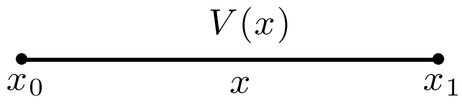
4.1. Single Axially Symmetric Branch with Arbitrary Tapering

For a single branch with center x along an interval $[x_0,x_1]$, possibly having geometric amplifying or dampening, the voltage and current density/voltage ratio are given by

$$\begin{array}{ccc}\hfill V\left(x\right)& =& \frac{C\left(x_1-x\right)+B\left(x_1\right)S\left(x_1-x\right)}{C\left(x_1-x_0\right)+B\left(x_1\right)S\left(x_1-x_0\right)}V\left(x_0\right)\hfill \\ & =& \left(C\left(x_1-x\right)+B\left(x_1\right)S\left(x_1-x\right)\right)V\left(x_1\right),\hfill \end{array}$$

(27)

$$B\left(x\right)=\frac{C^{\prime }\left(x_1-x\right)+B\left(x_1\right)S^{\prime }\left(x_1-x\right)}{C\left(x_1-x\right)+B\left(x_1\right)S\left(x_1-x\right)}=-\frac{V^{\prime }\left(x\right)}{V\left(x\right)},$$

(28)

respectively (see Figure 1).

Figure 1. A single branch with tapering.

Figure 1. A single branch with tapering.

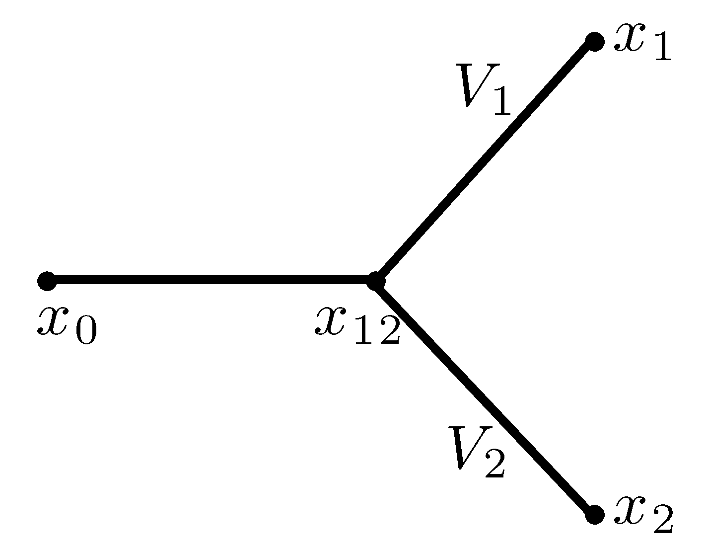
4.2. Junction of Three Branches with Different Types of Tapering

We now consider a general case in which each branch has its own geometry, possibly including amplification or dampening, assuming that the internal potential and current are assumed to be continuous at all branch points and at the soma-dendritic junction [14]. Assume there is a main branch with radius $r=r\left(x\right)$ and daughter branches with respective radii $r_1=r_1\left(x\right)$ and $r_2=r_2\left(x\right)$ (see Figure 2) and voltages represented by V, $V_1$ and $V_2$, respectively. If the point at which they join is called $x_{12}$, then

$$V\left(x_{12}\right)=V_1\left(x_{12}\right)=V_2\left(x_{12}\right),$$

(29)

and

$$r^2\left(x_{12}\right)B\left(x_{12}\right)=r_1^2\left(x_{12}\right)B_1\left(x_{12}\right)+r_2^2\left(x_{12}\right)B_2\left(x_{12}\right).$$

(30)

Figure 2. A junction of three different branches.

Figure 2. A junction of three different branches.

The total ratio constant $B\left(x_{12}\right)$ at the branching point $x_{12}$ is then given by

$$\begin{array}{ccc}\hfill B\left(x_{12}\right)& =& B\left(B_1\left(x_1\right),B_2\left(x_2\right)\right),\hfill \\ \mathrm{(31)}& & =& \frac{r_1^2\left(x_{12}\right)}{r^2\left(x_{12}\right)}{B}_1\left(x_{12}\right)+\frac{r_2^2\left(x_{12}\right)}{r^2\left(x_{12}\right)}{B}_2\left(x_{12}\right),\hfill & =& \frac{r_1^2\left(x_{12}\right)}{r^2\left(x_{12}\right)}\frac{C_1^{\prime }\left(x_1-x_{12}\right)+B_1\left(x_1\right)S_1^{\prime }\left(x_1-x_{12}\right)}{C_1\left(x_1-x_{12}\right)+B_1\left(x_1\right)S_1\left(x_1-x_{12}\right)}\hfill \\ & +& \frac{r_2^2\left(x_{12}\right)}{r^2\left(x_{12}\right)}\frac{C_2^{\prime }\left(x_2-x_{12}\right)+B_2\left(x_2\right)S_2^{\prime }\left(x_2-x_{12}\right)}{C_2\left(x_2-x_{12}\right)+B_2\left(x_2\right)S_2\left(x_2-x_{12}\right)}.\end{array}$$

Then $B\left(x_0\right)$ is a constant of the form:

$$B\left(x_0\right)=\frac{C^{\prime }\left(x_{12}-x_0\right)+B\left(x_{12}\right)S^{\prime }\left(x_{12}-x_0\right)}{C\left(x_{12}-x_0\right)+B\left(x_{12}\right)S\left(x_{12}-x_0\right)},$$

(32)

with the coefficient $B\left(x_{12}\right)$ found from Equation (31).

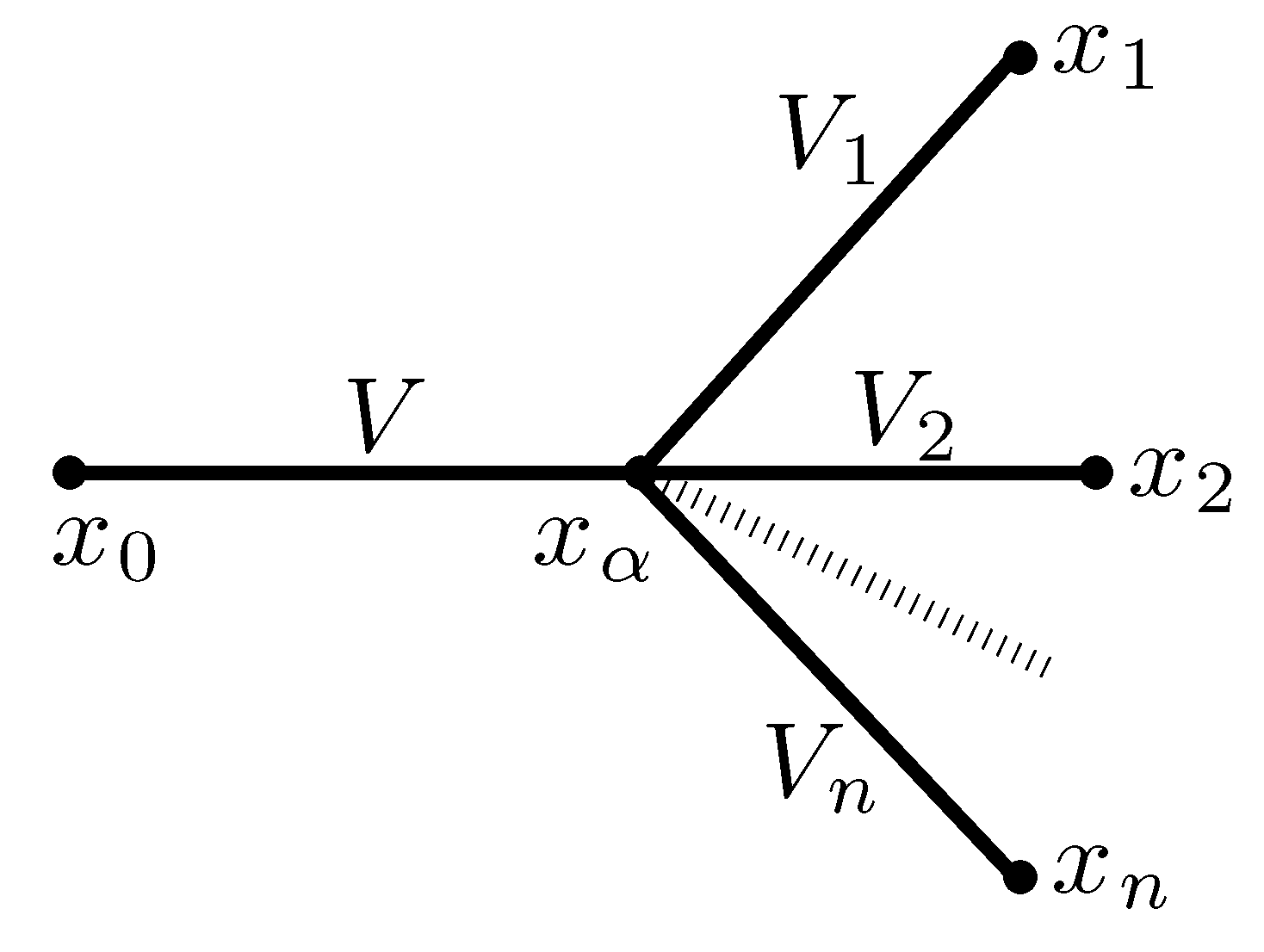
4.3. Junction of n-daughter branches

In a similar fashion (see Figure 3), at a branching point $x_{\alpha }$ giving rise to n daughter branches with potentials $V_i$, $i=1,...,n$ from an originating branch with potential V,

$$V\left(x_{\alpha }\right)=V_1\left(x_{\alpha }\right)=V_2\left(x_{\alpha }\right)=...=V_n\left(x_{\alpha }\right),$$

(33)

and

$$\begin{array}{ccc}\hfill r^2\left(x_{\alpha }\right)B\left(x_{\alpha }\right)& =& \sum _{i=1}^n{r}_i^2\left(x_{\alpha }\right)B_i\left(x_{\alpha }\right).\hfill \end{array}$$

Figure 3. A junction of $(n+1)$-branches.

Figure 3. A junction of $(n+1)$-branches.

A combination of the above graphical rules results in a simple algorithm for the evaluation of voltages and currents in the tree model. In short, first evaluate constants $B\left(x_{\alpha }\right)$ for all branching points of the tree and then, apply equation (31) for all open nodes. Finally, remove the above nodes from the tree and keep repeating the previous step until you reach the root of the tree.

In order to find voltage at a point x of the dendritic tree, follow the path from $x_0$ to x and multiply the initial voltage $V\left(x_0\right)$ by the consecutive corresponding factors from equation (27), changing at each branching point in the tree. The ratio of voltages $V\left(x_{\alpha }\right)$ and $V\left(x_{\beta }\right)$ at two terminal points $x_{\alpha }$ and $x_{\beta }$ can be determined by the previous graphical rule applied to the shortest path between $x_{\alpha }$ and $x_{\beta }$.

5. Examples

Equations (31) and (32) define the ratio coefficients $B\left(x_{\alpha }\right)$ for all vertices from the standard node on Figure 2. For the corresponding voltages, one can write

$$\begin{array}{ccc}\mathrm{(34)}& \hfill V\left(x_0\right)& =& \left[C\left(x_{12}-x_0\right)+B\left(x_{12}\right)S\left(x_{12}-x_0\right)\right]V\left(x_{12}\right),\hfill & =& \left[C\left(x_{12}-x_0\right)+B\left(x_{12}\right)S\left(x_{12}-x_0\right)\right]V\left(x_{12}\right)\hfill \\ & & \times \left[C\left(x_1-x_{12}\right)+B\left(x_1\right)S\left(x_1-x_{12}\right)\right]V\left(x_1\right),\hfill \\ & =& \left[C\left(x_{12}-x_0\right)+B\left(x_{12}\right)S\left(x_{12}-x_0\right)\right]V\left(x_{12}\right)\times \left[C\left(x_2-x_{12}\right)+B\left(x_2\right)S\left(x_2-x_{12}\right)\right]V\left(x_2\right),\hfill \end{array}$$

and

$$\frac{V\left(x_1\right)}{V\left(x_2\right)}=\frac{C\left(x_2-x_{12}\right)+B\left(x_2\right)S\left(x_2-x_{12}\right)}{C\left(x_1-x_{12}\right)+B\left(x_1\right)S\left(x_1-x_{12}\right)}.$$

(35)

Further examples are left to the reader.

6. Transient Solutions

Extensions to transient solutions for a single branch with tapering are covered in the following sections.

6.1. A Single Branch with Smooth Tapering

Now, consider the cable Equation (5) for a single branch with an arbitrary smooth tapering $r=r\left(x\right)$ on the interval $x_0\le x\le x_1.$ The separation of variables

$$V\left(x,t\right)=e^{-\left(1+{\alpha }^2\right)t/{\tau }_m}U\left(x\right),{\tau }_m=C_m{R}_m,$$

(36)

results in

$$\frac{1}{r}\frac{d}{dx}\left(r^2\frac{dU}{dx}\right)+{\omega }^2\frac{ds}{dx}U=0,{\omega }^2=\frac{2R_i}{R_m}{\alpha }^2,$$

(37)

where α is a separation constant. The boundary condition at the sealed-end condition (7) takes the form

$${\left.\left(\frac{dU}{dx}-\frac{1}{2}{\omega }^{2}U\right)\right|}_{x=x_1}=0.$$

(38)

A general solution of this problem for each branch of the tree can be conveniently written as

$$U\left(x\right)=U\left(x,\omega \right)=A\left[C\left(x,\omega \right)+\frac{1}{2}{\omega }^{2}S\left(x,\omega \right)\right]$$

(39)

where A is a constant and $C(x,\omega )$ and $S(x,\omega )$ are two linearly-independent standard solutions of Equation (37) that satisfy special boundary conditions $C(x_1,\omega )=1$, $C^{\prime }(x_1,\omega )=0$, and $S(x_1,\omega )=0$, $S^{\prime }(x_1,\omega )=1$. Then, the boundary condition Equation (8) at the somatic end $x=x_0$ is

$${\left.\left(\frac{dU}{dx}+\left[\frac{R_i}{R_s}\left(\frac{{\tau }_s}{{\tau }_m}-1\right)+\frac{C_s}{2C_m}{\omega }^2\right]U\right)\right|}_{x=x_0}=0,{\tau }_s=C_s{R}_s,$$

(40)

which results in a transcendental equation for the eigenvalues (ω):

$$\left[1-\frac{{\tau }_s}{{\tau }_m}\left(1+\frac{R_m}{2R_i}{\omega }^2\right)\right]\frac{R_i}{R_s}=\frac{C^{\prime }\left(x_0,\omega \right)+\frac{1}{2}{\omega }^2{S}^{\prime }\left(x_0,\omega \right)}{C\left(x_0,\omega \right)+\frac{1}{2}{\omega }^{2}S\left(x_0,\omega \right)}.$$

(41)

Note that there are infinitely many discrete eigenvalues for this equation [64,68]. The corresponding eigenfunctions $U_n=U\left(x,{\omega }_n\right)=A_n{u}_n\left(x\right)$ are orthogonal with respect to an inner product defined in terms of a Lebesgue–Stieltjes integral [64] (see also Appendix and [69,73,74]). In other words,

$$\left(u_m,u_n\right)={\delta }_{mn}\left(u_n,u_n\right),$$

(42)

where

$$(u,v)={\int }_{x_0}^{x_1}u\left(x\right)v\left(x\right)r\left(x\right)ds+\frac{1}{2}{r}^2\left(x_1\right)u\left(x_1\right)v\left(x_1\right)+\frac{C_s}{2C_m}{r}^2\left(x_0\right)u\left(x_0\right)v\left(x_0\right).$$

(43)

As a consequence,

$$V(t,x)=V(\infty ,x)+\sum _n{A}_{n}exp\left[-\left(1+\frac{R_m}{2R_i}{\omega }_n^2\right)\frac{t}{{\tau }_m}\right]u_n\left(x\right)$$

(44)

is a formal solution of the corresponding initial value problem where $V(\infty ,x)$ is the steady-state solution, where $\omega ={\omega }_n$ are roots of the transcendental equation (41) and the corresponding eigenfunctions are given by

$$u_n\left(x\right)=C\left(x,{\omega }_n\right)+\frac{1}{2}{\omega }_n^{2}S\left(x,{\omega }_n\right).$$

(45)

The coefficients $A_n$, $n=1,2,...$, can be obtained using the modified orthogonality relation (42) so that,

$$A_n=\frac{\left(V\left(x,0\right)-V\left(x,\infty \right),u_n\left(x\right)\right)}{\left(u_n\left(x\right),u_n\left(x\right)\right)}$$

(46)

(see the methods in [27,64]). Substitution of equation (46) into equation (44) and changing the order of summation and integration result in

$$V(t,x)=V(\infty ,x)+{\int }_{\text{Supp}\mu }G(t,x,y)\left(V(0,y)-V(\infty ,y)\right)d\mu \left(y\right),$$

(47)

where

$$G(t,x,y)=\sum _{n}exp\left[-\left(1+\frac{R_m}{2R_i}{\omega }_n^2\right)\frac{t}{{\tau }_m}\right]\frac{u_n\left(x\right)u_n\left(y\right)}{{∥u_n∥}^2},$$

(48)

is an analog of the heat kernel. This implies an infinite speed of propagation. The method of images and other standard methods can be applied for a tree with branching.

6.2. Single Branch with Piecewise Tapering

In the piecewise tapering case,

$$r=\left\{\begin{array}{cc}{r}_0\left(x\right),& x_0\le x\le x_{01}\hfill \\ r_1\left(x\right),& x_{01}\le x\le x_1\hfill \end{array}\right.$$

(49)

with $r_0\left(x_{01}^{-}\right)=r_1\left(x_{01}^{+}\right)$. In a similar fashion,

$$U\left(x,\omega \right)=\left\{\begin{array}{cc}{A}_0\left[C_0\left(x,\omega \right)-\left(\frac{R_i}{R_s}\left(\frac{{\tau }_s}{{\tau }_m}-1\right)+\frac{C_s}{2C_m}{\omega }^2\right)S_0\left(x,\omega \right)\right],\hfill & x_0\le x\le x_{01}\hfill \\ A_1\left[C_1\left(x,\omega \right)+\frac{1}{2}{\omega }^2{S}_1\left(x,\omega \right)\right],\hfill & x_{01}\le x\le x_1\hfill \end{array}\right.$$

(50)

assuming that $C_0(x_0,\omega )=1$, $C_0^{\prime }(x_0,\omega )=0$, and $S_0(x_0,\omega )=0$, $S_0^{\prime }(x_0,\omega )=1$, and $C_1(x_1,\omega )=1$, $C_1^{\prime }(x_1,\omega )=0$ and $S_1(x_1,\omega )=0$, $S_1^{\prime }(x_1,\omega )=1$. Continuity and smoothness of the solution at the point $x_{01}$,

$$\frac{U^{\prime }\left(x_{01}^{-}\right)}{U\left(x_{01}^{-}\right)}=\frac{U^{\prime }\left(x_{01}^{+}\right)}{U\left(x_{01}^{+}\right)},$$

(51)

results in the following equation for the eigenvalues

$$\frac{C_0^{\prime }\left(x_{01},\omega \right)-\left(\frac{R_i}{R_s}\left(\frac{{\tau }_s}{{\tau }_m}-1\right)+\frac{C_s}{2C_m}{\omega }^2\right)S_0^{\prime }\left(x_{01},\omega \right)}{C_0\left(x_{01},\omega \right)-\left(\frac{R_i}{R_s}\left(\frac{{\tau }_s}{{\tau }_m}-1\right)+\frac{C_s}{2C_m}{\omega }^2\right)S_0\left(x_{01},\omega \right)}=\frac{C_1^{\prime }\left(x_{01},\omega \right)+\frac{1}{2}{\omega }^2{S}_1^{\prime }\left(x_{01},\omega \right)}{C_1\left(x_{01},\omega \right)+\frac{1}{2}{\omega }^2{S}_1\left(x_{01},\omega \right)}.$$

(52)

Therefore, is possible to obtain a formal solution in the form of equations (47)–(48) once again by introducing

$$u_n\left(x\right)=\left\{\begin{array}{cc}{u}_n^{\left(0\right)}\left(x\right)/u_n^{\left(0\right)}\left(x_{01}\right),& x_0\le x\le x_{01}\\ u_n^{\left(1\right)}\left(x\right)/u_n^{\left(1\right)}\left(x_{01}\right),& x_{01}\le x\le x_1,\end{array}\right.$$

(53)

where

$$\begin{array}{ccc}\hfill u_n^{\left(0\right)}\left(x\right)& =& C_0\left(x,{\omega }_n\right)-\left(\frac{R_i}{R_s}\left(\frac{{\tau }_s}{{\tau }_m}-1\right)+\frac{C_s}{2C_m}{\omega }_n^2\right)S_0\left(x,{\omega }_n\right),\hfill \\ \hfill u_n^{\left(1\right)}\left(x\right)& =& C_1\left(x,{\omega }_n\right)+\frac{1}{2}{\omega }^2{S}_1\left(x,{\omega }_n\right).\hfill \end{array}$$

Further details are left to the reader.

7. Summary

We propose a simple graphical approach to steady-state solutions of the cable equation for a general model of a dendritic or axonal tree with tapering. A simple case of transient solutions is also briefly discussed. Possible future studies include numerical implementation of the methods described here to neuronal reconstructions.

References

1. Barret, J.N.; Crill, W.E. Influence of dendritic location and membrane properties on the effectiveness of synapses on cat motoneurones. J. Physiol. 1974, 239, 326–345. [Google Scholar] [CrossRef]
2. Holmes, W.R.; Rall, W. Electrotonic length estimates in neurons with dendritic tapering or somatic shunt. J. Neurophysiol. 1992, 68, 1421–1437. [Google Scholar] [PubMed]
3. Rall, W. Electrophysiology of a dendritic neuron model. Biophy. J. 1962, 2, 145–167. [Google Scholar] [CrossRef]
4. Rall, W.; Burke, R.E.; Smith, T.G.; Nelson, P.G.; Frank, K. Dendritic location of synapses and possible mechanisms for the monosynaptic EPSP in motoneurons. J. Neurophysiol. 1967, 30, 884–915. [Google Scholar]
5. Rall, W.; Shepherd, G.M.; Reese, T.S.; Brightman, M.W. Dendrodendritic synaptic pathway for inhibition in the olfactory bulb. Exp. Neurol. 1966, 14, 44–56. [Google Scholar] [CrossRef]
6. Rinzel, J.; Wilfrid, R. Transient response in a dendritic neuron model for current injected at one branch. Biophy. J. 1974, 14, 759–790. [Google Scholar] [CrossRef]
7. Stuart, G.J.; Häusser, M. Dendritic coincidence detection of EPSPs and action potentials. Nature Neurosci. 2001, 4, 63–71. [Google Scholar] [CrossRef] [PubMed]
8. Baer, S.M.; Tier, C. An analysis of a dentric neuron model with an active membrane site. J. Math. Biol. 1986, 23, 137–161. [Google Scholar] [CrossRef] [PubMed]
9. Häusser, M.; Spruston, N.; Stuart, G.J. Diversity and dynamics of dendritic signaling. Science 2000, 290, 739–744. [Google Scholar] [CrossRef] [PubMed]
10. Migliore, M.; Shepherd, G.M. Emerging rules for the distributions of active dendritic conductances. Nature Rev. Neurosci. 2002, 3, 362–370. [Google Scholar] [CrossRef] [PubMed]
11. Sakatani, S.; Hirose, A. The influence of neuron shape changes on the firing characteristics. Neurocomputing 2003, 52, 355–362. [Google Scholar] [CrossRef]
12. Vetter, P.; Ross, A.; Hausser, M. Propagation of action potential in dendrites depends on dendritic morphology. J. Neurophysiol. 2001, 85, 926–937. [Google Scholar] [PubMed]
13. Kelvin, L. On the theory of the electric telegraph. Proc. Roy. Soc. (London) 1855, 7, 382. [Google Scholar]
14. Rall, W. Branching dendritic trees and motoneurons membrane resistivity. Exp. Neurol. 1959, 1, 491–527. [Google Scholar] [CrossRef]
15. Rall, W. Methods in Neuronal Modeling; MIT Press: Cambridge, MA, USA, 1989; pp. 9–92. [Google Scholar]
16. Rall, W. Core conductor theory and cable properties of neurons. In Comprehensive Physiology; Wiley: Hoboken, NJ, USA, 2011; pp. 39–97. [Google Scholar]
17. Rall, W. Membrane potential transients and membrane time constant of motoneurons. Exp. Neurol. 1960, 2, 503–532. [Google Scholar] [CrossRef]
18. Rall, W. Theory of physiological properties of dendrites. Ann. N. Y. Acad. Sci. 1962, 96, 1071–1092. [Google Scholar] [CrossRef] [PubMed]
19. Rall, W. Time constants and electrotonic length of membrane cylinders and neurons. Biophy. J. 1969, 9, 1483–1508. [Google Scholar] [CrossRef]
20. Rall, W.; Rinzel, J. Branch input resistance and steady attenuation for input to one branch of a dendritic neuron model. Biophys. J. 1973, 13, 648–688. [Google Scholar] [CrossRef]
21. Evans, J.D. Analytical solution of the cable equation with synaptic reversal potential for passive neurones with tip-to-tip dendrodendric coupling. Math. Biosci. 2005, 196, 125–152. [Google Scholar] [CrossRef] [PubMed]
22. Ohme, M.; Schierwagen, A. An equivalent cable model for neuronal trees with active membrane. Biol. Cybernetics 1998, 78, 227–243. [Google Scholar] [CrossRef]
23. Major, G.; Evans, J.D.; Jack, J.J. Solutions for transients in arbitrarily branching cables: I. Voltage recording with a somatic shunt. Biophy. J. 1993, 65, 423–449. [Google Scholar] [CrossRef]
24. Major, G.; Evans, J.D.; Jack, J.J.B. Solutions for transients in arbitrarily branching cables: II. Voltage clamp theory. Biophy. J. 1993, 65, 450–468. [Google Scholar] [CrossRef]
25. Major, G. Solutions for transients in arbitrarily branching cables: III. Voltage clamp problems. Biophy. J. 1993, 65, 469–491. [Google Scholar] [CrossRef]
26. Major, G.; Evns, J.D. Solutions for transients in arbitrarily branching cables: IV. Nonuniform electrical parameters. Biophy. J. 1993, 66, 615–633. [Google Scholar] [CrossRef]
27. Durand, D. The somatic shunt cable model for neurons. Biophys. J. 1984, 46, 645–653. [Google Scholar] [CrossRef]
28. Evans, J.D.; Kember, G.C.; Major, G. Techniques for obtaining analytical solutions to the multicylinder somatic shunt cable model for passive neurones. Biophys. J. 1992, 63, 350–365. [Google Scholar] [CrossRef]
29. Cox, S.J.; Raol, J.H. Recovering the passive properties of tapered dendrites from single and dual potential recordings. Math. Biosci. 2004, 190, 9–37. [Google Scholar] [CrossRef] [PubMed]
30. Tsay, D.; Yuste, R. Role of dendritic spines in action potential backpropagation: A numerical simulation study. J. Neurophysiol. 2002, 88, 2834–2845. [Google Scholar] [CrossRef] [PubMed]
31. Baer, S.; Tier, C. Techniques for obtaining analytical solutions for Rall’s model neuron. J. Neurosci. Methods 1987, 20, 151–166. [Google Scholar]
32. Coombes, S.; Timofeeva, Y.; Svensson, C.M.; Lord, G.J.; Josić, K.; Cox, S.J.; Colbert, C.M. Branching dendrites with resonant membrane: A “sum-over-trips” approach. Biol. Cybernatics 2007, 97, 137–149. [Google Scholar] [CrossRef] [PubMed]
33. Roth, A.; Häusser, M. Compartmental models of rat cerebellar Purkinje cells based on simultaneous somatic and dendritic patch-clamp recordings. J. Physiol. 2001, 535, 445–472. [Google Scholar] [CrossRef] [PubMed]
34. Häusser, M.; Mel, B. Dendrites: bug or feature? Curr. Opin. Neurobiol. 2003, 13, 372–383. [Google Scholar] [CrossRef]
35. Krichmar, J.L.; Nasuto, S.J.; Scorcioni, R.; Washington, S.D.; Ascoli, G.A. Effects of dendritic morphology on CA3 pyramidal cell electrophysiology: A simulation study. Brain Res. 2002, 941, 11–28. [Google Scholar] [CrossRef]
36. Mainen, Z.F.; Sejnowski, T.J. Influence of dendritic structure on firing pattern in model neocortical neurons. Nature 1996, 382, 363–366. [Google Scholar] [CrossRef] [PubMed]
37. Nevian, T.; Larkum, M.E.; Polsky, A.; Schiller, J. Properties of basal dendrites of layer 5 pyramidal neurons: A direct patch-clamp recording study. Nature Neurosci. 2007, 10, 206–214. [Google Scholar] [CrossRef] [PubMed]
38. Surkis, A.; Taylor, B.; Peskin, C.S.; Leonard, C.S. Quantitative morphology of physiologically identified and intracellularly labeled neurons from the guinea-pig laterodorsal tegmental nucleus in vitro. Neuroscience 1996, 74, 375–392. [Google Scholar] [CrossRef]
39. Rall, W. Membrane time constant of motoneurons. Science 1957, 126, 454. [Google Scholar] [CrossRef] [PubMed]
40. Abrikosov, A.A.; Gorkov, L.P.; Dzyaloshinski, I.E. Methods of Quantum Field Theory in Statistical Physics; Dover Publications: New York, NY, USA, 1963. [Google Scholar]
41. Akhiezer, A.; Berestetskii, V.B. Quantum Electrodynamics; Interscience Publishers: New York, NY, USA, 1965. [Google Scholar]
42. Berestetskii, V.B.; Lifshitz, E.M.; Pitaevskii, L.P. Relativistic Quantum Theory; Pergamon Press: Oxford, UK, 1971. [Google Scholar]
43. Feynman, R.P. The theory of positrons. Phys. Rev. 1949, 76, 749–759. [Google Scholar] [CrossRef]
44. Feynman, R.P. Space-time approach to quantum electrodynamics. Phys. Rev. 1949, 76, 769–789. [Google Scholar] [CrossRef]
45. Feynman, R.P. QED: The Strange Theory of Light and Matter; Princeton, N.J., Ed.; Princeton University Press: Princeton, NJ, USA, 1985. [Google Scholar]
46. Kaiser, D. Physics and Feynman’s diagrams. Am. Sci. 2005, 93, 156–165. [Google Scholar] [CrossRef]
47. Mattuck, R.D. A Guide to Feynmann Diagrams in theMany-Body Problems; Dover Publications: New York, NY, USA, 1992. [Google Scholar]
48. Weinberg, S. The Quantum Theory of Fields; Cambridge University Press: Cambridge, UK, 1998; Volumes 1–3. [Google Scholar]
49. Meiler, M.; Cordero-Soto, R.; Suslov, S.K. Solution of the Cauchy problem for a time-dependent Schrödinger equation. J. Math. Phys. 2008, 49, 072102. [Google Scholar] [CrossRef]
50. Nikiforov, A.F.; Suslov, S.K.; Uvarov, V.B. Classical Orthogonal Polynomials of a Discrete Variable; Springer–Verlag: Berlin, Germany; New York, NY, USA, 1991. [Google Scholar]
51. Smirnov, Y.F.; Shitikova, K.V. The method of Kharmonics and the shell model. Sov. J. Part. Nucl. 1977, 8, 344–370. [Google Scholar]
52. Smorodinskii, Y.A. Trees and many-body problem. Izv. Vyssh. Uchebn. Zaved. Radiofiz. 1976, 19, 932–941. [Google Scholar] [CrossRef]
53. Abbott, L.F. Simple diagrammatic rules for solving dendritic cable problems. Physica A 1992, 185, 343–356. [Google Scholar] [CrossRef]
54. Chruściński, D.; Jurkowski, J. Memory in a nonlocally damped oscillator. In Proceedings of Quantum Bio-Informatics III From Quantum Information to Bio-Informatics, Tokyo, Japan, 11–14 March 2009.
55. Cordero-Soto, R.; Lopez, R.M.; Suazo, E.; Suslov, S.K. Propagator of a charged particle with a spin in uniform magnetic and perpendicular electric fields. Lett. Math. Phys. 2008, 84, 159–178. [Google Scholar] [CrossRef]
56. Cordero-Soto, R.; Suazo, E.; Suslov, S.K. Models of damped oscillators in quantum mechanics. J. Phy. Math. 2009, 1, S090603. [Google Scholar] [CrossRef]
57. Cordero-Soto, R.; Suazo, E.; Suslov, S.K. Quantum integrals of motion for variable quadratic Hamiltonians. Ann. Phys. 2010, 315, 1884–1912. [Google Scholar] [CrossRef]
58. Cordero-Soto, R.; Suslov, S.K. Time reversal for modified oscillators. Theo. Math. Phy. 2010, 162, 286–316. [Google Scholar] [CrossRef]
59. Lanfear, N.; Suslov, S.K. The ime-dependent Schrödinger Equation, Riccati Equation and Airy Functions. Available online: http://arxiv.org/pdf/0903.3608.pdf (accessed on 22 April 2009).
60. Suazo, E.; Suslov, S.K.; Vega-Guzmán, J.M. The Riccati differential equation and a diffusion-type equation. N. Y. J. Math. 2011, 17, 225–244. [Google Scholar]
61. Suslov, S.K. Dynamical invariants for variable quadratic Hamiltonians. Phys. Scr. 2010, 81, 055006. [Google Scholar] [CrossRef]
62. Jack, J.J.B.; Noble, D.; Tsien, R.W. Electric Current Flow in Excitable Cells; Oxford University Press: Oxford, UK, 1975. [Google Scholar]
63. Foster, A.; Hendryx, E.; Murillo, A.; Salas, M.; Morales-Butler, E.J.; Suslov, S.K.; Herrera-Valdez, M. Extensions of the Cable Equation Incorporating Spatial Dependent Variations in Nerve Cell Diameter. Available online: http://mtbi.asu.edu/research/archive (accessed on 31 August 2010).
64. Churchill, R.V. Expansions in series of non-orthogonal functions. Bull. Amer. Math. Soc. 1942, 48, 143–149. [Google Scholar] [CrossRef]
65. Abramowitz, M.; Stegan, I.A. Handbook of Mathematical Functions; Dover Publications: New York, NY, USA, 1972. [Google Scholar]
66. Andrews, G.E.; Askey, R.A.; Roy, R. Special Functions; Cambridge University Press: Cambridge, UK, 1999. [Google Scholar]
67. Askey, R.A. Orthogonal Polynomials and Special Functions. In Proceedings of the CBMS–NSF Regional Conferences Series in Applied Mathematics, SIAM, Philadelphia, PA, USA, 1 June 1975.
68. Hartman, P. Ordinary Differential Equations; John Wiley & Sons: Baltimore, MA, USA, 1973. [Google Scholar]
69. Kellogg, O.D. Note on closure of orthogonal sets. Bull. Amer. Math. Soc. 1921, 27, 165–169. [Google Scholar] [CrossRef]
70. Kolmogorov, A.N.; Fomin, S.V. Introductory Real Analysis; Dover: New York, NY, USA, 1970; pp. 1–365. [Google Scholar]
71. Nikiforov, A.F. Lectures on Equations and Methods of Mathematical Physics; Intellect: Dolgoprudnii, Russia, 2009. (in Russian) [Google Scholar]
72. Nikiforov, A.F.; Uvarov, V.B. Special Functions of Mathematical Physics; Birkhäuser: Basel, Boston, 1988. [Google Scholar]
73. Reid, W.T. A boundary value problem assiciated with the calculus of variations. Am. J. Math. 1932, 54, 769–790. [Google Scholar] [CrossRef]
74. Reid, W.T. Oscillation criteria for self-adjoint differential systems. Trans. Amer. Math. Soc. 1961, 101, 91–106. [Google Scholar] [CrossRef]
75. Erdélyi, A. Higher Transcendental Functions, Volumes I–III; Erdélyi, A., Ed.; McGraw-Hill: New York, NY, USA, 1953. [Google Scholar]
76. Olver, F.W.J. Asymptotics and Special Functions; Academic Press: New York, NY, USA, 1974. [Google Scholar]
77. Rainville, E.D. Special Functions; The Macmillan Company: New York, NY, USA, 1960. [Google Scholar]
78. Vilenkin, N.Y. Special Functions and the Theory of Group Representations; American Mathematical Society: Providence, RI, USA, 1968. [Google Scholar]
79. Watson, G.N. A Treatise on the Theory of Bessel Functions, 2nd ed.; Cambridge University Press: Cambridge, UK, 1944. [Google Scholar]