
Finite-Time Stabilization of Homogeneous Non-Lipschitz Systems


1
Polytechnical School of Tunisia, B.P. 743, La Marsa 2078, Tunis, Tunisia
2
LAIMI Laboratory, University of Quebec at Chicoutimi, Chicoutimi, QC G7H 2B1, Canada
*
Author to whom correspondence should be addressed.
Mathematics 2016, 4(4), 58; https://doi.org/10.3390/math4040058
Submission received: 17 June 2016
/
Revised: 22 August 2016
/
Accepted: 13 September 2016
/
Published: 24 September 2016
Abstract
:This paper focuses on the problem of finite-time stabilization of homogeneous, non-Lipschitz systems with dilations. A key contribution of this paper is the design of a virtual recursive Hölder, non-Lipschitz state feedback, which renders the non-Lipschitz systems in the special case dominated by a lower-triangular nonlinear system finite-time stable. The proof is based on a recursive design algorithm developed recently to construct the virtual Hölder continuous, finite-time stabilizer as well as a C1 positive definite and proper Lyapunov function that guarantees finite-time stability of the non-Lipschitz nonlinear systems.

1. Introduction
In the 1990s, thanks to the differential geometric approach, several techniques appeared to design a systematic feedback insuring global asymptotic stabilization and robust control of systems [1,2,3]. Among them, a Lyapunov-based recursive design technique was created, called backstepping, which consisted of a recursive adding a power integrator. Originally proposed by Coran and Praly [4], this technique presented certain limitations due to necessary conditions imposed on the system [2,5,6]. Recently, a synthesis derived technique, called the desingularizing method [7], based on the homogeneous system theory [4,8,9,10], was investigated by [11,12] in designing a recursive algorithm providing the construction of state feedback controllers and a Lyapunov function. The importance of system homogeneity stems from the fact that it has useful properties like equivalence between local asymptotic stability and global asymptotic stability for linear homogeneous systems. Furthermore, different results and characteristics were obtained in the past decades, studying nonlinear homogeneous systems [3,13,14]. Therefore, for simplicity, as well as keeping applications in mind, we focused on continuous homogeneous lower-triangular nonlinear systems.
In the works [15,16], finite-time stabilizers were derived by using the theory of homogeneous systems. Moreover, due to the use of a homogeneous approximation, only local finite-time stabilization results can be established for specific cases of nonlinear systems such as the homogeneous lower-triangular nonlinear systems with applications on two- to three-dimensional control systems [15,17,18,19]. Motivated by the above discussion, our concern was to develop a finite-time controller, relying on the Lyapunov theory for finite-time stability to achieve global finite-time stabilization for non-Lipshitz, n-dimensional homogeneous lower-triangular nonlinear systems. Therefore, we proposed a new constructive methodology based on adding a power integrator, inspired by recent works [11,20,21,22], with a convergence speed improvement suggested in [23] and the idea of homogeneous-based Lyapunov functions.
Recently, in the literature, the authors in [24] developed systematic algorithms to design both non-Hölder and Hölder continuous state feedback and a control Lyapunov function, to achieve global finite-time stabilization for a class of uncertain nonlinear systems. A non-Hölder, controller and a control Lyapunov function was proposed to globally finite-time stabilize a class of nonlinear cascaded system in [22]. In the higher dimension case, such as in [25] a Hölder, continuous state feedback control laws achieved local finite-time stabilization for triangular systems and for certain classes of nonlinear systems. The fact is that the issue of global finite-time stabilization of n-dimensional nonlinear systems can be achieved by Hölder; however, state feedback still remains unknown and unanswered.
The novelty of our contribution comes, then, from a new tool which is based on a methodical algorithm. This tool evolves a recursive mathematical relation between the Hölder exponents and the dilation coefficients, using the convexity property derived from our assumptions. Moreover, we show, using a step-by-step resized and reconstructed subsystem, how to explicitly design a virtual, Hölder, non-Lipschitz state feedback control law. This control law is able to stabilize, in finite-time, a lower-triangular homogeneous nonlinear system as well as homogeneous-based Lyapunov functions, in the form that we will give later when we will formulate our main theorem with a useful hypothesis.
To the best knowledge of the authors, there is no study on this new Hölder controller, nor the Lyapunov function form defined by our Theorem. As an application, a feedback control law is designed based on this Lyapunov function for three main systems: the single, double and triple integrators.
This paper is organized as follows. In Section 2, we introduce the concept of finite-time stability of continuous autonomous systems. We state the new theorem, which is the main result of this paper, and give the most important definitions and lemmas, that will be used in the sequel. In Section 3, we demonstrate, with some detailed proofs, the different steps for the construction of the algorithm. Finally, for proving the convergence in finite-time with the feedback law established in this work, the effectiveness of the proposed algorithm is shown in Section 4 with a design example and a computer simulation.
2. Preliminary Results
2.1. Finite-Time Stability
This section gives some basic concepts and terminologies related to the notion of finite-time stability and the corresponding Lyapunov stability theory. We also recall the Lyapunov theorem of finite-time stability, which gives a necessary and sufficient condition for non-Lipschitz continuous autonomous systems to be finite-time stable [15,18,19,26,27].
Definition 1.
(Bhat and Bernstein 2000 [19]) Consider the non-Lipschitz continuous autonomous system on the open neighborhood D of the origin , , such that
The equilibrium of the system (1) is finite-time convergent if there are an non empty opened neighborhood U of the origin and a function , such that every solution trajectory of (1) starting from the initial point is defined on and . T is called the settling-time of the initial state . The equilibrium of (1) is finite-time stable if it is Lyapunov stable and finite-time convergent. If , the origin is a globally finite-time stable equilibrium.
It has also been demonstrated, with the Proposition 2.3 in [19], that if the origin is a finite-time stable equilibrium of (1), then the system (1) has a unique solution on , for every initial condition in an open neighborhood of 0, including 0 itself. The reader can note that only non-smooth or non-Lipschitz continuous autonomous systems have the property of finite-time stability convergence, whereby the solution trajectory of a non-Lipschitzian system reaches a Lyapunov stable equilibrium state (the origin in finite time). Let us introduce the concept of finite-time stabilizability by the next definition.
Definition 2.
(Finite-time stabilizability) The controlled system
is stabilizable in finite-time, if there exists a continuous feedback law vanishing at the origin such that 0 is stable in finite-time for the closed-loop system .
The following theorem provides sufficient conditions for the origin of the system (1) to be a finite-time stable equilibrium.
Theorem 1.
(Finite-time stability) Consider the non-Lipschitz continuous autonomous system (1). Suppose there is function defined on a neighborhood of the origin, and real numbers and , such that
- is positive definite on and
- , .
Then, the origin of system (1) is locally finite-time stable. The settling time, depending on the initial state , satisfies, for all in some open neighborhood of the origin:
If and is also radially unbounded, the origin of system (1) is globally finite-time stable.
2.2. Finite-Time Stabilizing Feedback
In this section, we state a theorem, the main result of this paper, in order to provide a recursive algorithm to design a Hölderian continuous state feedback, under certain conditions, which renders the homogeneous non-Lipschitz closed-loop system globally finite-time stabilizable. For more convenience, we define as the set of all rational numbers, whose numerators and denominators are all positive and odd integers.
Theorem 2.
We consider the class of nonlinear homogeneous systems in the lower triangular form
We assume that , such that , are functions vanishing at the origin and homogeneous of degree , . Let be a decreasing sequence in , such that
where is the Hölder exponent of the Lyapunov function associated with the system (1), such that , for and the dilation coefficient of the system (1), satisfying
and the iterative relation
where such that and , for . Then, there exists a feedback controller with , which renders the origin of the closed-loop system finite-time stable.
We introduce the next Lemmas, which will be used in the proof of Theorem 2.
Lemma 1.
The next Lemmas are a direct consequence of the Young’s inequality [20].
Lemma 3.
For any positive real numbers and , the following inequality holds
Lemma 4.
Let a and b be any real numbers and , and then
Lemma 5.
Let c, d be positive real numbers and a real-valued function, then
3. Proof of Theorem 2
In order to prove Theorem 2, a modified backstepping procedure is used, which simultaneously enables the construction of a positive definite and proper control Lyapunov function, as well as a non-Lipschitz finite-time feedback control law rendering the closed-loop system (3), which is finite-time stable. Different Lemmas and demonstrated propositions will be used during the progression of the proof.
It should be noted that the constructive proof is given by induction, and the structure is similar to [3,11,24,28]. For the first step of the induction, we choose the Lyapunov function that is positive definite, proper and with a Hölder exponent
with the convention that . Using (11) and Lemma 1, we can find, by a simple derivative computation, a smooth function such that
Using Lemma 2, we can deduce as that
Therefore, we can write
By taking a smooth non-negative function, such that
we then have . If we choose to take the virtual control as follows,
with a smooth positive function, it yields
Inductive assumption: Suppose that at the th step, there is a proper and positive definite Lyapunov function for the system (3) and a set of virtual controllers defined by the form
where are smooth positive functions, such that
To prove the induction at the kth step, we consider the Lyapunov function defined by
where .
The next proposition that we are using is available for the set of all rationales in . It was used in [28] for the same technique, and one can be referred to [29,30] for the proof.
Proposition 1.
and are functions, and we have the following results:
We can then deduce from the inequality (18), that
In order to refine the previous inequality, we investigate each term of Equation (21) one by one. Using Lemma 4 and knowing that , we can write the inequality
Then, we deduce using Lemma 5 that
where is an adequate fixed constant. To continue the estimation of the inequality (21), we introduce the next propositions.
Proposition 2.
For , there are positive functions , such that
Proof.
Using the fact that , we can write
Using Lemma 3 and the fact that and , we have for :
where is a chosen positive function satisfying two conditions given later in the following demonstration (see Equation (39)). ☐
Proposition 3.
For , there are positive functions , such that
Proof.
We have the next estimation, for , using Lemma 1, Lemma 4 and that , with :
where is a chosen positive function. ☐
For the estimation of the term , we use an inductive argument as described in the following.
For the first step, we note that there exists a positive function obviously verifying
Inductive assumption For , there exist smooth positive functions such that
We want to prove that for , there are positive functions , such that
We also know that ; then, for , we can calculate and obtain:
where we have adopted, for more convenience, the notation
For the last step, we prove that Equation (29) holds for . Recalling that does not depend on , we calculate the derivative form
with an adequate chosen smooth positive function.
Finally, using Equations (28) and (31) with the fact that , we deduce the next inequality for ,
We estimate the parts of the Equations A and B by the following
Then, by adding Equations (33) and (34), we can write :
where , , and are positive smooth functions. Using both Lemma 1 and 5, we estimate the next term of the inequality (21):
Using the inequality , we obtain
Knowing that , , we have
We impose in addition, when constructing to the smooth positive function , to satisfy the two conditions below:
Therefore, we have for
where is a smooth positive function. Finally, for the last term of (21), there exists a smooth positive function such that
To prove this claim, we start with the next inequality:
Using the fact that and Lemma 4, we can write
Combining the result obtained in Equation (43), with Proposition 3 and Lemma 5 yields:
where is a positive smooth function. Substituting the estimates Equations (23), (40) and (41) into Equation (21) yields:
A plausible choice of a continuous Hölderian virtual controller is then given by:
Then, the correspondent Lyapunov function satisfies:
which completes the proof of the inductive step. Using the inductive argument above, we conclude that at the nth step, there exists a non-Lipschitz continuous state feedback control law of the form:
where is a positive function and a positive definite and proper Lyapunov function constructed by the inductive procedure verifying the inequality:
This completes the proof of the inductive step.
Using Theorem 1, one can verify that the system (3) is globally finite-time stable [24]. As a consequence and under the necessary and sufficient conditions of Theorem 2, we have shown that the closed-loop homogeneous nonlinear system in the form (3) is finite-time stabilizable by a Hölderian non-Lipshitz continuous feedback, as long as , are functions with .
Finally, we propose in the next section, an example to illustrate our design scheme and validate the results obtained.
4. Simulations of the Controller
Different results of finite-time controller designing have been already obtained with different techniques and methodologies [15,23,24,26,27,31,32]. Since the proposed theorem gives a new form for the Lyapunov function, the effectiveness of the algorithm developed in this paper is demonstrated with a design example and a computer simulation for the three common cases: the single, double and triple integrators. For the first step, , which defined the single integrator, we choose to work with the positive definite Lyapunov function . In addition, we choose to take , , and , which leads to a virtual control with the following form:
It should be noted that the feedback law stabilizes the simple integrator , as shown in Figure 1, with the initial condition .
In the following steps, we notice that our main Theorem (2) gives us two frame relations to help us to find and as they have to satisfy:
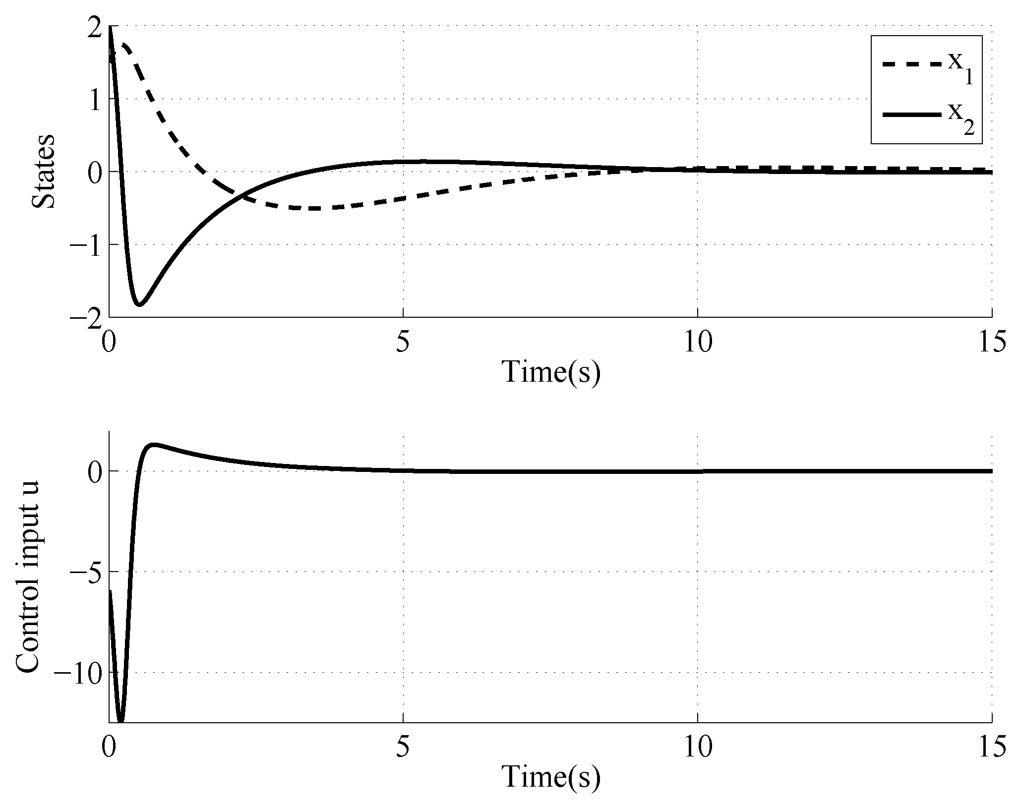
For the second step, , we choose to take , and . The corresponding virtual control , is given by the form:
As shown in Figure 2, this feedback law also stabilizes the double integrator , in response to the initial conditions .
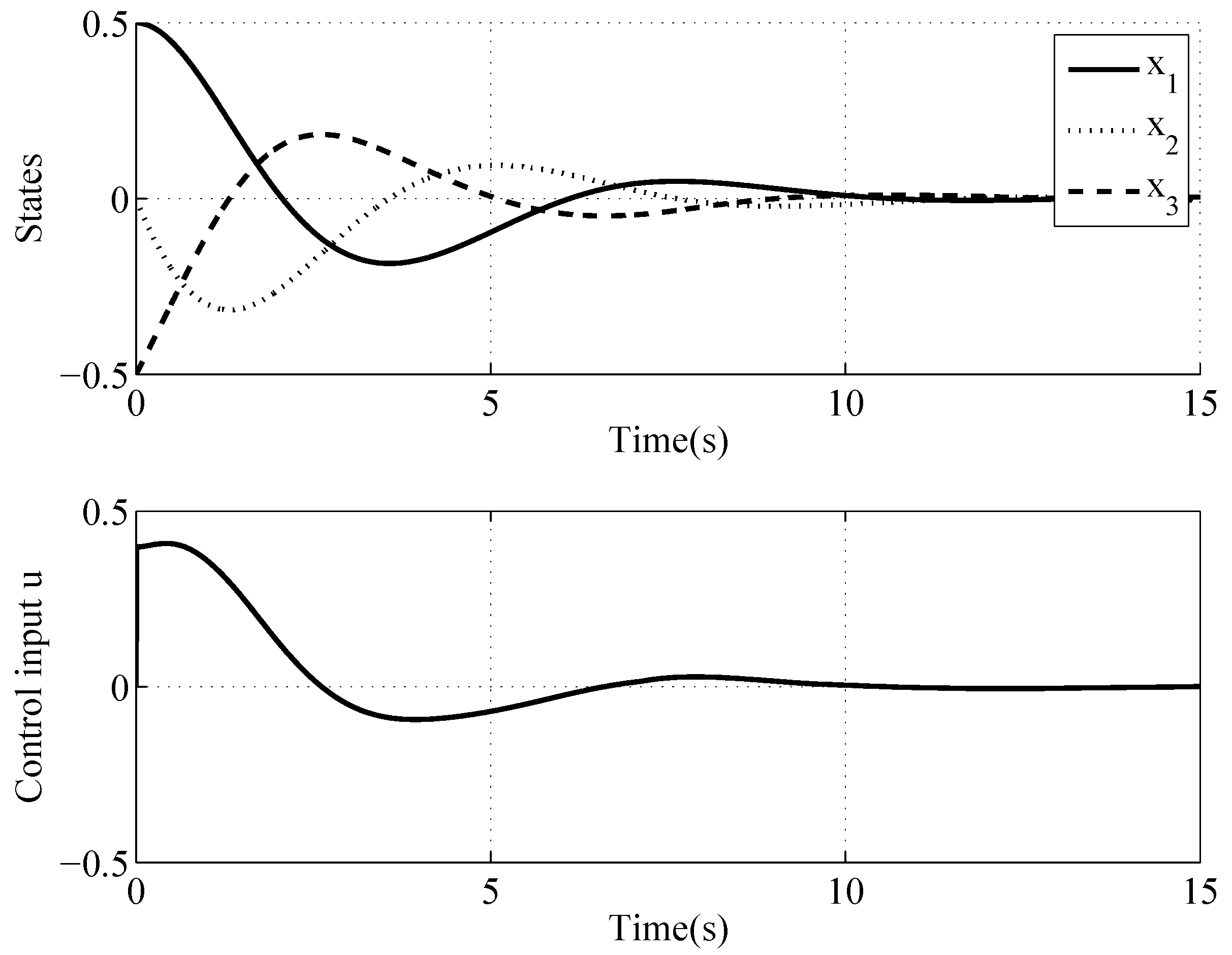
For the final step, , we choose to take , and . The corresponding virtual control is given by the form:
Figure 3 shows that the triple integrator——is stabilized in response to the initial conditions .
5. Conclusions
In this paper, we have extended the notion of finite-time stability to homogeneous non-Lipschitz systems, especially in the case of the lower-triangular nonlinear systems, using a systematic recursive algorithm, achieving the design of virtual continuous non-Lipschitz finite-time stabilizing controllers as well as control Lyapunov functions, under appropriate conditions. The advantage of this algorithm is that it uses a recursive relation between the dilation coefficients and the Hölder-exponents, to determine, step by step, the virtual Hölder feedback and the Lyapunov function, performing the finite-time stabilization task of the considered class of systems.
Finally, we have demonstrated the effectiveness and convenience of the proposed procedure illustrated by computer simulations on simple, double and triple integrator models, insuring finite-time stability and Lyapunov functions determinations.
In further works, we will be interested by a more developed class of nonlinear systems such as fractional systems, unknown parameter systems, and ones subject to disturbance. Since some applications could be found in a robotic control field, we will focus on the Human–Robot interaction model as shown in [33,34,35] and on the interesting problematic of finite-time stability frontier under critical values of impedance like damping and mass parameters, especially in the case where the states of the system are subject to disturbance.
Acknowledgments
This work was supported in part by the Natural Sciences and Engineering Research Council of Canada (NSERC), under the grant number 418235-2012.
Author Contributions
Nawel Khelil designed the control algorithm and wrote this journal paper. Martin J.-D. Otis has been involved in revising it critically for important intellectual content. Also, he has given final approval of the version to be published.
Conflicts of Interest
The authors declare no conflict of interest.
References
- Byrnes, C.I.; Isidori, A. Asymptotic stabilization of minimum phase nonlinear systems. IEEE Trans. Autom. Control 1991, 36, 1122–1137. [Google Scholar] [CrossRef]
- Isidori, A. Nonlinear Control Systems 2; Springer: New York, NY, USA, 1999. [Google Scholar]
- Palendo, J.; Qian, C. A generalized framework for global output feedback stabilization of genuinely nonlinear systems. In Proceedings of the 44th IEEE Conference on Decision and Control and European Control Conference (CDC-ECC 2005), Seville, Spain, 12–15 December 2005; pp. 2646–2651.
- Coron, J.M.; Praly, L. Adding an integrator for the stabilization problem. Syst. Control Lett. 1991, 17, 89–104. [Google Scholar] [CrossRef]
- Byrnes, C.I.; Isidori, A. New results and examples in nonlinear feedback stabilization. Syst. Control Lett. 1989, 12, 437–442. [Google Scholar] [CrossRef]
- Lin, W.; Qian, C. Adding one power integrator: A tool for global stabilization of higher order lower-triangular system. Syst. Control Lett. 2000, 39, 339–351. [Google Scholar] [CrossRef]
- Praly, L.; Andrea-Novel, B.; Coron, J.M. Lyapunov design of stabilizing controllers for cascaded systems. IEEE Trans. Autom. Control 1991, 36, 1177–1181. [Google Scholar] [CrossRef]
- Bacciotti, A. Local Stabilizability of Nonlinear Control Systems; World Scientific: Singapore, 1992. [Google Scholar]
- Hermes, H. Homogeneous coordinates and continuous asymptotically stabilizing feedback controls. In Differential Equations Stability and Control; Elaydi, S., Ed.; Marcel Dekker: New York, NY, USA, 1991; pp. 249–260. [Google Scholar]
- Kawski, M. Homogeneous stabilizing feedback laws. Control Theory Adv. Technol. 1990, 6, 497–516. [Google Scholar]
- Qian, C.; Lin, W. Non-Lipschitz continuous stabilizers for nonlinear systems with uncontrollable unstable linearization. Syst. Control Lett. 2001, 42, 185–200. [Google Scholar] [CrossRef]
- Ding, S.; Li, S.; Zheng, W. Nonsmooth stabilization of a class of non linear cascaded systems. Automatica 2012, 48, 2597–2606. [Google Scholar] [CrossRef]
- Andreini, A.; Bacciotti, A.; Stefani, G. Global stabilizability of homogeneous vector fields of odd degree. Syst. Control Lett. 1988, 10, 251–256. [Google Scholar] [CrossRef]
- Qian, C. A homogeneous domination approach for global output feedback stabilization of a class of nonlinear systems. In Proceedings of the 2005 American Control Conference, Portland, OR, USA, 8–10 June 2005; Volume 7, pp. 4708–4715.
- Bhat, S.P.; Bernstein, D.S. Continuous finite-time stabilization of the translational and rotational double intergrator. IEEE Trans. Autom. Control 1998, 43, 678–682. [Google Scholar] [CrossRef]
- Hong, Y.; Huang, J.; Xu, Y. On an output feedback finite-time stabilization problem. IEEE Trans. Autom. Control 2001, 46, 305–309. [Google Scholar] [CrossRef]
- Bhat, S.P.; Bernstein, D.S. Lyapunov analysis of finite-time differential equations. In Proceedings of the American Control Conference, Seattle, WA, USA, 21–23 June 1995; Volume 3, pp. 1831–1832.
- Bhat, S.P.; Bernstein, D.S. Finite-time stability of homogeneous systems. In Proceedings of the American Control Conference, Albuquerque, NM, USA, 4–6 June 1997; Volume 4, pp. 2513–2514.
- Bhat, S.P.; Bernstein, D.S. Finite-time stability of continuous autonomous systems. SIAM J. Control Optim. 2000, 38, 751–766. [Google Scholar] [CrossRef]
- Yang, B. Output Feedback Control for Nonlinear Sytems with Unstabilizable and Undetectable Linearization. Ph.D. Thesis, Case Western Reserve University, Cleveland, OH, USA, August 2006. [Google Scholar]
- Qian, C.; Lin, W. Non-Smooth stabilizers for nonlinear systems with uncontrollable unstable linearization. In Proceedings of the 39th IEEE Conference on Decision and Control, Sydney, Australia, 12–15 December 2000; Volume 2, pp. 1655–1660.
- Qian, C.; Lin, W. A continuous feedback approach to global strong stabilization of nonlinear systems. IEEE Trans. Autom. Control 2001, 46, 1061–1079. [Google Scholar] [CrossRef]
- Shen, Y.; Huang, Y. Global finite-time stabilisation for a class of nonlinear systems. Int. J. Syst. Sci. 2012. [Google Scholar] [CrossRef]
- Huang, X.; Lin, W.; Yang, B. Global finite-time stabilization of a class of uncertain nonlinear systems. Automatica 2005, 41, 881–888. [Google Scholar] [CrossRef]
- Hong, Y. Finite-time stabilization and stabilizability of a class of controllable systems. Syst. Control Lett. 2002, 46, 231–236. [Google Scholar] [CrossRef]
- Jammazi, C. Finite-time partial stabilizability of chained systems. Comptes Rendus Math. 2008, 346, 975–980. [Google Scholar] [CrossRef]
- Jammazi, C. On a sufficient condition for finite-time partial stability and stabilization: Applications. IMA J. Math. Control Inf. 2010, 27, 29–56. [Google Scholar] [CrossRef]
- Back, J.; Cheong, S.G.; Shim, H.; Seo, J.H. Nonsmooth feedback stabilizer for strict-feedback nonlinear systems that may not be linearizable at the origin. Syst. Control Lett. 2007, 56, 742–752. [Google Scholar] [CrossRef]
- Nakamura, H.; Yamashita, Y.; Nishitani, H. Homogeneous eigenvalue analysis of homogeneous systems. In Proceedings of the 16th IFAC World Congress, Prague, Czech, 3–8 July 2005.
- Nakamura, H.; Yamashita, Y.; Nishitani, H. Stabilization of homogeneous systems using implicit control Lyapunov functions. In Proceedings of the 7th IFAC Symposium on Nonlinear Control Systems, Pretoria, South Africa, 21–24 August 2007; Volume 7, pp. 561–566.
- Bhat, S.P.; Bernstein, D.S. Geometric homogeneiy with applicatons to finite-time stability. Math. Control Signals Syst. 2005, 17, 101–127. [Google Scholar] [CrossRef]
- Ding, S.; Li, S.; Li, Q. Stability analysis for a second order continuous finite-time control system subject to a disturbance. J. Control Theory Appl. 2009, 7, 271–276. [Google Scholar]
- Duchaine, V.; Gosselin, C.M. Investigation of Human-Robot interaction stability using Lyapunov theory. In Proceedings of the IEEE International Conference in Robotics and Automation, Pasadena, CA, USA, 19–28 May 2008; pp. 2189–2194.
- Campeau-Lecours, A.; Otis, M.J.-D.; Belzile, P.-L.; Gosselin, C. A time-domain vibration observer and controller for physical human-robot interaction. Mechatronics 2016, 36, 45–53. [Google Scholar] [CrossRef]
- Meziane, R.; Li, P.; Otis, M.J.-D.; Ezzaidi, H.; Cardou, P. Safer hybrid workspace using human-robot interaction while sharing production activities. In Proceedings of the IEEE International Symposium on Robotic and Sensors Environments (ROSE), Timisoara, Romania, 16–18 October 2014; pp. 37–42.
Figure 1.
Initial condition response of a finite-time stabilized simple integrator.
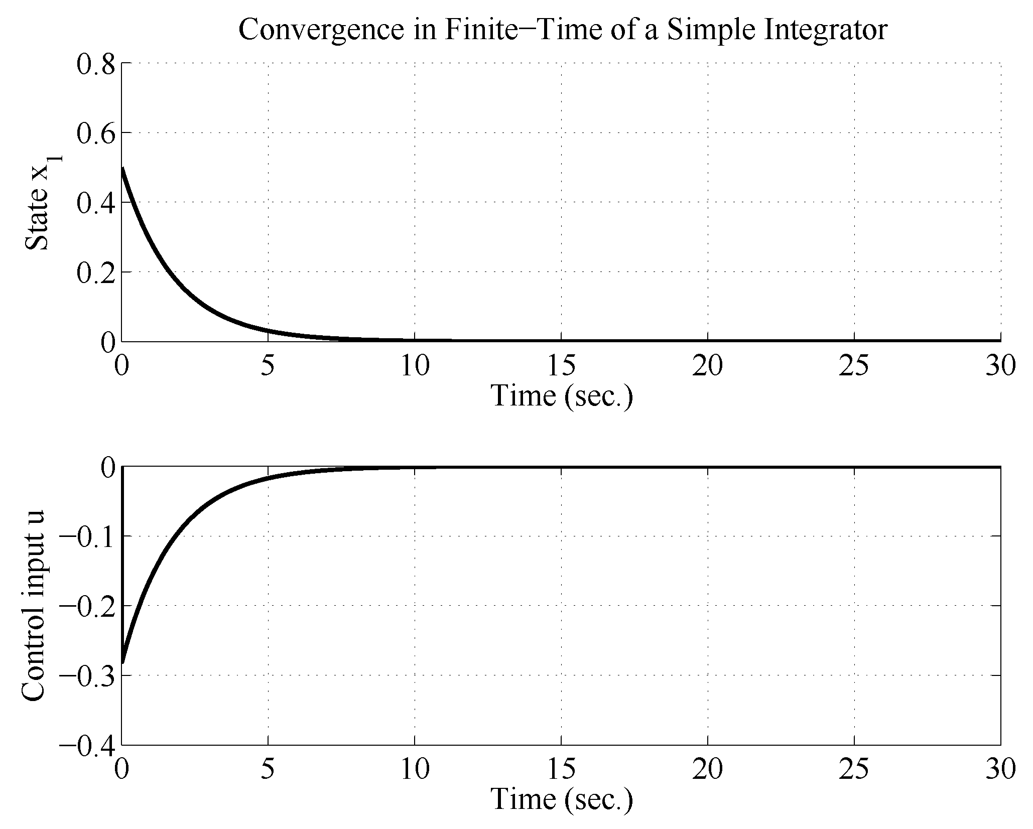
Figure 2.
Initial condition response of a finite-time stabilized double integrator.

Figure 3.
Initial condition response of a finite-time stabilized triple integrator.
© 2016 by the authors; licensee MDPI, Basel, Switzerland. This article is an open access article distributed under the terms and conditions of the Creative Commons Attribution (CC-BY) license (http://creativecommons.org/licenses/by/4.0/).
Share and Cite
MDPI and ACS Style
Khelil, N.; Otis, M.J.-D. Finite-Time Stabilization of Homogeneous Non-Lipschitz Systems. Mathematics 2016, 4, 58. https://doi.org/10.3390/math4040058
AMA Style
Khelil N, Otis MJ-D. Finite-Time Stabilization of Homogeneous Non-Lipschitz Systems. Mathematics. 2016; 4(4):58. https://doi.org/10.3390/math4040058
Chicago/Turabian StyleKhelil, Nawel, and Martin J.-D. Otis. 2016. "Finite-Time Stabilization of Homogeneous Non-Lipschitz Systems" Mathematics 4, no. 4: 58. https://doi.org/10.3390/math4040058
Note that from the first issue of 2016, this journal uses article numbers instead of page numbers. See further details here.