1. Introduction
A series of interesting and unusual properties of the state-of-the art low-dimensional quantum systems requires new approaches in mathematical modeling by means of the Schrödinger equation. Different generalizations of the standard Schrödinger equation by introducing either time fractional derivatives or space fractional derivatives have been introduced for this reason [
1,
2,
3,
4,
5,
6,
7,
8,
9,
10,
11,
12,
13,
14]. It has been shown that their solutions can be represented by using the Mittag-Leffler (M-L) and Fox
H-functions. In our recent work [
15], we considered time-dependent Schrödinger equation with memory kernel and we show that such generalized equation contains many already investigated special cases, such as standard Schrödinger equation, time fractional Schrödinger equation with Caputo fractional derivative, and distributed order Schrödinger equation. We also show that the probability distribution function
is not conserved. In [
5], an effective potential is introduced in the standard Schrödinger equation and it is shown that this approach is equivalent to the time fractional Schrödinger equation with Caputo fractional derivative (see also [
16]) giving the wave function of the same form. The effective potential approach is of great importance for elucidating for example, dissipative quantum transport processes in quantum dots [
17,
18]. This motivates us to further extend and upgrade the quantum transport modeling by means of generalized Schrödinger equation.
In the present paper, we derive a general form of the imaginary effective potential which, at same boundary conditions, relates the standard Schrödinger equation to the generalized Schrödinger equation with a memory kernel. Throughout the paper, the solutions with separable variables are analyzed. We show that by using the appropriately derived effective potential, one may consider a generalized Schrödinger equation with a memory kernel instead of the standard time-dependent Schrödinger equation. The advantage of this approach is that the solutions of generalized Schrödinger equation can be represented in an elegant manner by means of the M-L and Fox H-functions, enabling a comprehensive mathematical modeling for a wide class of problems. We further derive the explicit form of effective potential for several memory kernels, such as Dirac delta, power-law, Mittag-Leffler and truncated power-law memory kernels, expressing the effective potential in terms of the M-L functions. The results obtained in this work provide a strong mathematical basis for modeling and simulations of problems related to inelastic scattering, such as dissipative quantum transport in low-dimensional quantum systems. As the limitations of the conventional approaches in both, mathematical modeling and simulations of the state-of-the-art applications are evident, introducing the imaginary effective potential is expected to contribute to a more sophisticated insight of such problems.
This paper is organized as follows. In
Section 2 we give some results for the generalized Schrödinger equation with memory kernel. The standard Schrödinger equation with an effective potential is analyzed in
Section 3. The effective potential for which the standard Schrödinger equation has same solution as the one for the generalized Schrödinger equation is obtained. For different forms of the memory kernel we derive the effective potential in terms of the M-L functions and infinite series in three parameter M-L functions. The summary is given in
Section 4.
2. Generalized Schrödinger Equation
In our recent work [
15], we analyze time-dependent Schrödinger-like equation with memory kernel which in the force free case is given by
where
is integrable memory kernel for which the assumption of form
,
is satisfied. It is a corresponding equation to the generalized diffusion equation recently derived in [
19] from the generalized Langevin equation, and in [
20] from the continuous time random walk theory. It is shown that such equation contains a number of limiting cases, such as the standard Schrödinger equation for
, time fractional Schrödinger equation with Caputo fractional derivative for
,
, and distributed order Schrödinger equation in case where the memory kernel is of distributed order [
15]. The constraints for the memory kernel
under which the solution of the generalized diffusion equation represents a probability distribution function are analyzed in [
20,
21]. Furthermore, comb models with generalized memory kernels are analyzed in [
21] as well.
By using the separation ansatz
, it is shown that [
15]
where
λ is the separation constant that corresponds to the energy, from where it follows
In [
15] we showed that, in general, the probability distribution function
is time-dependent, and a rich variety of behaviors may be obtained depending on the choice performed to
, in particular a power-law decay. In this sense, the analyzis performed here has a particular case the one presented in Reference [
5] for a time fractional Schrödinger equation which may correspond to a choice of
.
In the paper by Bayin [
5], the time fractional Schrödinger equation with the Caputo time fractional derivative was considered, and it was shown that the wave function of the equation in the force free case can be obtained if one considers the standard Schrödinger equation with an effective potential, which can be considered as a possible physical interpretation of the fractional Schrödinger equation.
In what follows, we try to find the standard Schrödinger equation which solution is a same as the one of Equation (
1), by finding the corresponding effective potential. Some special cases for the memory kernel are investigated.
3. Effective Potential
Let us now consider the standard Schrödinger equation of form
where
is the so-called
effective potential [
5]. This effective potential is an analogue to the memory kernel in the generalized Schrödinger equation and they both describe dissipation. Namely, the problem of inelastic scattering of particles can be observed as a motion of a particle in an imaginary effective potential that enters in the standard time-dependent Schrödinger Equation (
6). By using the method of separation of variables, and by using a spatial solution (
5), we obtain that the effective potential has the following form
From solution (
4) for the effective potential finally we obtain
Thus, the standard Schrödinger Equation (
6) with effective potential of form (
8) has same solution for the wave function
as the one obtained for the generalized Schrödinger Equation (
1). From (
8), it follows that the time-dependent effective potential is also energy-dependent, involving the parametric integral dependence on the energy of the scattered particle. Thus, the effective potential here is obtained relative to the value of the energy
λ.
Let us now analyze some special cases for the memory kernel .
3.1. Standard Schrödinger Equation: Dirac Delta Memory Kernel
For the Dirac delta memory kernel
, i.e.,
, for the effective potential one can find
as it should be.
3.2. Time Fractional Schrödinger Equation: Power-Law Memory Kernel
For the power law memory kernel
,
, i.e.,
, for the effective potential we find
where
is the one parameter M-L function (see relation (
A1)). By using relation (
A3) in (
10) and then by applying relation (
A4), for the effective potential we derive
where
is the two parameter M-L function (see relation (
A1)). Note that for
the effective potential (
10) becomes zero as it is expected, since the time fractional Schrödinger equation turns to standard Schrödinger equation, i.e., the Caputo time fractional derivative becomes ordinary derivative.
3.3. Fractional Schrödinger Equation with Two Fractional Exponents: Two Power-Law Memory Kernels
If we further consider a memory kernel as a mix of two power-law functions
,
,
,
,
, i.e.,
, for the effective potential we obtain
or equivalently
where
is the three parameter M-L function (
A1). Here we used the series expansion approach [
22] and the Laplace transform relation (
A2). The series that appear in relation (
12) has been shown to be convergent [
23] (see also detailed study of the convergence of series in M-L functions in [
24,
25]). By using the asymptotic expansion formula (
A5) for the case with
, and
, one can easily derive the result (
11) for one power-law memory kernel. The same result (
11) is directly obtained from (
12) and (
13) for the case with
and
. Such bi-fractional Schrödinger equation has been recently investigated in [
26] in detail. This case can be considered as a distributed order Schrödinger equation where the weight function is a sum of two delta functions.
3.4. Mittag-Leffler Memory Kernel
Let us further consider two parameter M-L memory kernel of form
,
,
. Such memory kernel is recently considered in the diffusion equation with generalized memory kernels in the framework of the continuous time random walk theory [
20]. For
it becomes one parameter M-L memory kernel
, and for
– exponential memory kernel
. Note that for
the M-L memory kernel becomes a power-law memory kernel
. From the Laplace transform formula (
A2), it follows that
, so
. Thus, for the effective potential we find
For
, solution (
14) reduces to
and for
– to
Thus, for exponential memory kernel, the effective potential does not depend on time. Such complex potentials have been introduced to model open quantum dots [
27] and for simulation of resonant tunneling diode [
28]. It is known that for such imaginary potentials the current conservation for the electron state is not preserved due to the lack of unitarity of the Hamiltonian which includes complex potential [
29]. Note that in case where
, i.e., power-law memory kernel, the effective potential becomes
which corresponds to (
10) since
.
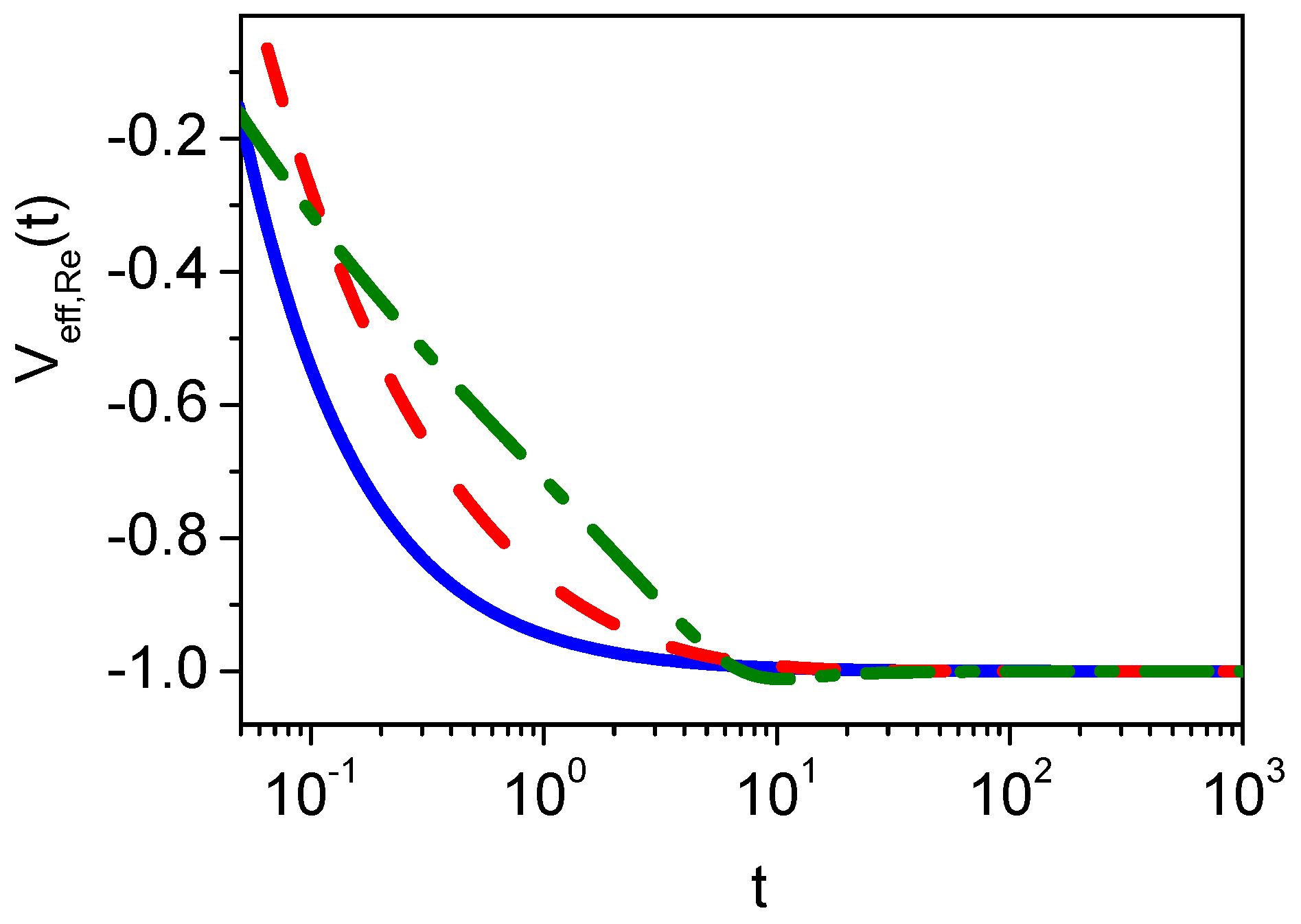
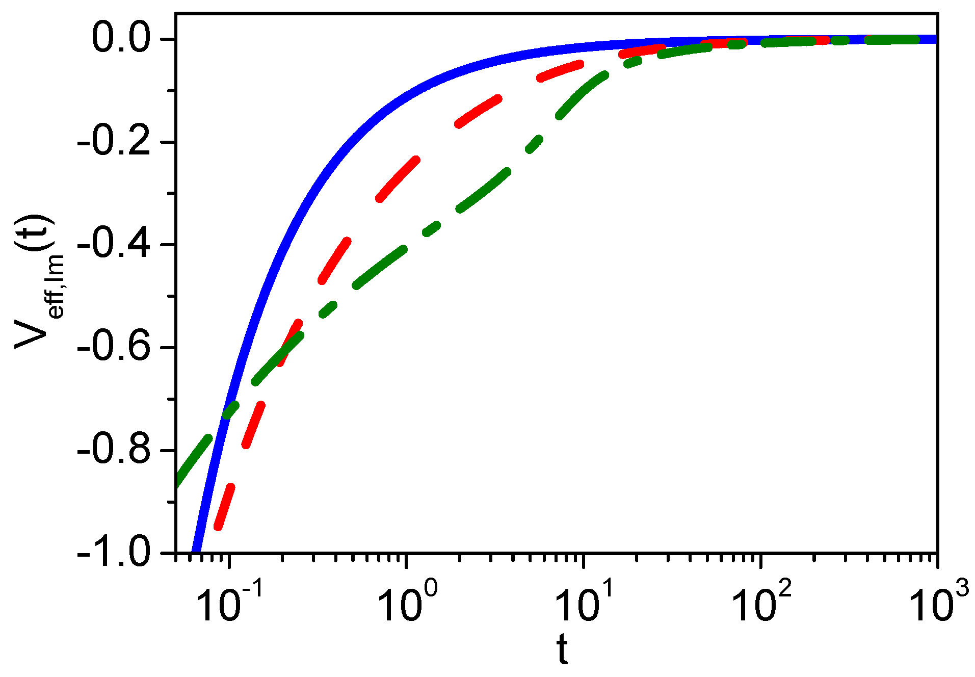
A graphical representation of the real and imaginary part of the effective potential (
14) is given in
Figure 1.
3.5. Truncated Power-Law Memory Kernel
Additionally, we consider a power-law memory kernel with an exponential cutoff, i.e., truncated power-law memory kernel of the form
where
,
, and
. From the Laplace transform formula and by help of the shift rule
, where
, we find that
from where one concludes that the assumption
. Therefore, for the effective potential we obtain
Note that for
, it follows
which is exactly the same with relation (
17), as it should be. Note that truncated M-L and power-law memory kernels are considered in the context of the CTRW theory in [
20], where it is shown that such memory kernel is useful to model processes where for short times anomalous subdiffusion exists, which turns to normal diffusion in the long time limit. Similar analysis for the effective potential in case of the truncated M-L memory kernel can be done here.
4. Summary
To summarize, in the present paper we derived a general form of the imaginary effective potential that relates the standard time-dependent Schrödinger equation to the generalized Schrödinger equation with a memory kernel. This provides an alternative mathematical framework for modeling the inelastic scattering-related problems, applicable in a wide variety of low-dimensional quantum systems. For example, dissipative quantum transport in quantum dots, as well as the decaying part in resonant tunneling could be successfully modeled by such imaginary potentials. In this work we also derived explicitly the imaginary potentials for some of the most exploited forms of the memory kernel, such as Dirac delta, power-law, M-L, exponential, truncated power-law. We further expressed the effective potentials in terms of the M-L functions. The importance of the results obtained here is many-fold. At one hand, using the generalized Schrödinger equation with a memory kernel, instead of standard time-dependent Schrödinger equation enables obtaining a closed form solutions, expressed in terms of the M-L and Fox H-functions, which contributes to a more sophisticated and consistent mathematical modeling. On the other hand, the derived imaginary effective potentials upgrade the set of conventional forms of scattering potentials and can be used as input potentials in dissipative transport simulations. Finally, it is worth mentioning that such an approach provides in-depth insight and an interpretation of the considered generalized Schrödinger equation.
Acknowledgments
T.S. acknowledges the hospitality and support from the Max Planck Institute for the Physics of Complex Systems in Dresden, Germany.
Author Contributions
All authors have contributed equally.
Conflicts of Interest
The authors declare no conflict of interest.
Appendix A. Mittag-Leffler Functions
Three parameter M-L function is defined by [
30]
One parameter M-L function
and two parameter M-L function
are special cases of three parameter M-L function if we use
and
, respectively. The Laplace transform to three parameter M-L function is given by [
30]
The following relations for the M-L functions hold true [
31]
For the three parameter M-L function one can use the following formula [
32,
33,
34]
from where it follows
for
. For
follows the known asymptotic formula for two parameter M-L function [
35]
References
- Naber, M. Time fractional Schrödinger equation. J. Math. Phys. 2004, 45, 3339. [Google Scholar] [CrossRef]
- Laskin, N. Fractional quantum mechanics and Lévy path integrals. Phys. Lett. A 2000, 268, 298–305. [Google Scholar] [CrossRef]
- Laskin, N. Fractional quantum mechanics. Phys. Rev. E 2000, 62, 3135. [Google Scholar] [CrossRef]
- Laskin, N. Fractional Schrödinger equation. Phys. Rev. E 2002, 66, 056108. [Google Scholar] [CrossRef] [PubMed]
- Bayin, S.S. Time fractional Schrödinger equation: Fox’s H-functions and the effective potential. J. Math. Phys. 2013, 54, 012103. [Google Scholar] [CrossRef]
- Ertik, H.; Demirhan, D.; Sirin, H.; Büyükkiliç, F. Time fractional development of quantum systems. J. Math. Phys. 2010, 51, 082102. [Google Scholar] [CrossRef]
- Jiang, X.; Qi, H.; Xu, M. Exact solutions of fractional Schrödinger-like equation with a nonlocal term. J. Math. Phys. 2011, 52, 042105. [Google Scholar] [CrossRef]
- Lenzi, E.K.; de Oliveira, B.F.; da Silva, L.R.; Evangelista, L.R. Solutions for a Schrödinger equation with a nonlocal term. J. Math. Phys. 2008, 49, 032108. [Google Scholar] [CrossRef]
- Liemert, A.; Kienle, A. Fractional Schrödinger equation in the presence of the linear potential. Mathematics 2016, 4, 31. [Google Scholar] [CrossRef]
- Luchko, Y. Fractional Schrödinger equation for a particle moving in a potential well. J. Math. Phys. 2013, 54, 012111. [Google Scholar] [CrossRef]
- Muslih, S.I. Solutions of a particle with fractional δ-potential in a fractional dimensional space. Int. J. Theor. Phys. 2010, 49, 2095–2104. [Google Scholar] [CrossRef]
- Lenzi, E.K.; Ribeiro, H.V.; Mukai, H.; Mendes, R.S. Continuous-time random walk as a guide to fractional Schrödinger equation. J. Math. Phys. 2010, 51, 092102. [Google Scholar]
- Narahari Achar, B.N.; Yale, B.T.; Hanneken, J.W. Time fractional Schrödinger equation revisited. Adv. Math. Phys. 2013, 2013, 290216. [Google Scholar]
- Iomin, A.; Sandev, T. Lévy transport in slab geometry of inhomogeneous media. Math. Model. Nat. Phenom. 2016, 11, 51–62. [Google Scholar] [CrossRef]
- Sandev, T.; Petreska, I.; Lenzi, E.K. Time-dependent Schrödinger-like equation with nonlocal term. J. Math. Phys. 2014, 55, 092105. [Google Scholar] [CrossRef]
- Dubbeldam, J.L.A.; Tomovski, Z.; Sandev, T. Space-time fractional Schrödinger equation with composite time fractional derivative. Fract. Calc. Appl. Anal. 2015, 18, 1179–1200. [Google Scholar] [CrossRef]
- Baraff, G.A. Model for the effect of finite phase-coherence length on resonant transmission and capture by quantum wells. Phys. Rev. B 1998, 58, 13799. [Google Scholar] [CrossRef]
- Ferry, D.K.; Baker, J.R.; Akis, R. Complex potentials, dissipative processes, and general quantum transport. In Proceedings of the 1999 International Conference on Modelling and Simulation of Micro Systems, NSTI (1999), San Juan, PR, USA, 19–21 April 1999; pp. 373–376.
- Tateishi, A.A.; Lenzi, E.K.; da Silva, L.R.; Ribeiro, H.V.; Picoli, S., Jr.; Mendes, R.S. Different diffusive regimes, generalized Langevin and diffusion equations. Phys. Rev. E 2012, 85, 011147. [Google Scholar] [CrossRef] [PubMed]
- Sandev, T.; Chechkin, A.; Kantz, H.; Metzler, R. Diffusion and Fokker-Planck-Smoluchowski equations with generalized memory kernel. Fract. Calc. Appl. Anal. 2015, 18, 1006–1038. [Google Scholar] [CrossRef]
- Sandev, T.; Iomin, A.; Kantz, H.; Metzler, R.; Chechkin, A. Comb model with slow and ultraslow diffusion. Math. Model. Nat. Phenom. 2016, 11, 18–33. [Google Scholar] [CrossRef]
- Podlubny, I. Fractional Differential Equations; Academic Press: San Diego, CA, USA, 1999. [Google Scholar]
- Sandev, T.; Tomovski, Z.; Dubbeldam, J.L.A. Generalized Langevin equation with a three parameter Mittag-Leffler noise. Phys. A 2011, 390, 3627–3636. [Google Scholar] [CrossRef]
- Paneva-Konovska, J. Convergence of series in three parametric Mittag-Leffler functions. Math. Slovaca 2014, 64, 73–84. [Google Scholar] [CrossRef]
- Paneva-Konovska, J. On the multi-index (3m-parametric) Mittag-Leffler functions, fractional calculus relations and series convergence. Cent. Eur. J. Phys. 2013, 11, 1164–1177. [Google Scholar] [CrossRef]
- Martins, J.; Ribeiro, H.V.; Evangelista, L.R.; da Silva, L.R.; Lenzi, E.K. Fractional Schrödinger equation with noninteger dimensions. Appl. Math. Comput. 2012, 219, 2313–2319. [Google Scholar] [CrossRef]
- Berggren, K.-F.; Yakimenko, I.I.; Hakanen, J. Modeling of open quantum dots and wave billiards using imaginary potentials for the source and the sink. New J. Phys. 2010, 12, 073005. [Google Scholar] [CrossRef]
- Sharifi, M.J.; Navi, K. Physic-based imaginary potential and incoherent current models for RTD simulation using optical model. J. Appl. Sci. 2008, 8, 1028–1034. [Google Scholar]
- Sun, J.P.; Haddad, G.I.; Mazumder, P.; Schulman, J.N. Resonant tunneling diodes: Models and properties. Proc. IEEE 1998, 86, 641–661. [Google Scholar]
- Prabhakar, T.R. A singular integral equation with a generalized Mittag-Leffler function in the kernel. Yokohama Math. J. 1971, 19, 7–15. [Google Scholar]
- Shukla, A.K.; Prajapati, J.C. On a generalization of Mittag-Leffler function and its properties. J. Math. Anal. Appl. 2007, 336, 797–811. [Google Scholar] [CrossRef]
- Saxena, R.K.; Mathai, A.M.; Haubold, H.J. Unified fractional kinetic equation and a fractional diffusion equation. Astrophys. Space Sci. 2004, 209, 299–310. [Google Scholar] [CrossRef]
- Sandev, T.; Tomovski, Z. Langevin equation for a free particle driven by power law type of noises. Phys. Lett. A 2014, 378, 1–9. [Google Scholar] [CrossRef]
- Sandev, T.; Metzler, R.; Tomovski, Z. Correlation functions for the fractional generalized Langevin equation in the presence of internal and external noise. J. Math. Phys. 2014, 55, 023301. [Google Scholar] [CrossRef]
- Mainardi, F. Fractional Calculus and Waves in Linear Viscoelesticity: An Introduction to Mathematical Models; Imperial College Press: London, UK, 2010. [Google Scholar]
© 2016 by the authors; licensee MDPI, Basel, Switzerland. This article is an open access article distributed under the terms and conditions of the Creative Commons Attribution (CC-BY) license (http://creativecommons.org/licenses/by/4.0/).


