
Interval Type 2 Fuzzy Set in Fuzzy Shortest Path Problem

1
Department of Computer Science and Engineering, Saroj Mohan Institute of Technology, Hooghly 712512, West Bengal, India
2
Department of Mathematics, National Institute of Technology, Durgapur 713209, West Bengal, India
3
Department of Computer Science and Engineering, National Institute of Technology, Durgapur 713209, West Bengal, India
*
Author to whom correspondence should be addressed.
Mathematics 2016, 4(4), 62; https://doi.org/10.3390/math4040062
Submission received: 10 March 2016
/
Revised: 13 September 2016
/
Accepted: 22 September 2016
/
Published: 9 October 2016
Abstract
:The shortest path problem (SPP) is one of the most important combinatorial optimization problems in graph theory due to its various applications. The uncertainty existing in the real world problems makes it difficult to determine the arc lengths exactly. The fuzzy set is one of the popular tools to represent and handle uncertainty in information due to incompleteness or inexactness. In most cases, the SPP in fuzzy graph, called the fuzzy shortest path problem (FSPP) uses type-1 fuzzy set (T1FS) as arc length. Uncertainty in the evaluation of membership degrees due to inexactness of human perception is not considered in T1FS. An interval type-2 fuzzy set (IT2FS) is able to tackle this uncertainty. In this paper, we use IT2FSs to represent the arc lengths of a fuzzy graph for FSPP. We call this problem an interval type-2 fuzzy shortest path problem (IT2FSPP). We describe the utility of IT2FSs as arc lengths and its application in different real world shortest path problems. Here, we propose an algorithm for IT2FSPP. In the proposed algorithm, we incorporate the uncertainty in Dijkstra’s algorithm for SPP using IT2FS as arc length. The path algebra corresponding to the proposed algorithm and the generalized algorithm based on the path algebra are also presented here. Numerical examples are used to illustrate the effectiveness of the proposed approach.
1. Introduction
The problem of finding the shortest path from a specified source node to a destination node is a fundamental and well known combinatorial optimization problem in graph theory. Many real world problems, e.g., transportation, communication, scheduling, economical system analysis, supply chain management, computer network, etc., can be modeled as an SPP. A common algorithm to solve the classical SPP is the Dijkstra’s algorithm [1,2].
In many applications such as urban traffic planning, routing of telecommunication messages, telemarketing operator scheduling, optimal pipelining of VLSI chip, texture mapping, etc., graphs emerge as a mathematical model of the observed real world system. Many problems can be reformulated as a quest for a path between two nodes in a graph which is optimal in the sense of a number of preset criteria. These optimality criteria are evaluated in terms of weights, i.e., vectors of real numbers, associated with the links of the graph. In a real-world model, an edge is associated with a direction and with a measure of impedance, determining the parameters, like time, cost, capacity, demand, traffic frequency, etc., along the network. In real life applications, like vehicle green routing and scheduling, transportation, etc., which are related to environmental issues, the arc lengths could be uncertain due to the fluctuation with traffic conditions or weather conditions, even if the geometric distance is fixed. Therefore finding the optimal path in such networks could be challenging. Fuzziness can be introduced into a network/graph to deal with this type of uncertain situations.
There are many efforts in FSPP [3,4,5,6,7,8,9,10,11,12,13,14,15,16,17] using T1FS. An algorithm for FSPP was proposed first by Dubois and Prade [3] based on the extension of the classical Floyd and Ford-Moore-Bellman (FMB) algorithms. They introduced the idea of criticality of a path. Given a fuzzy number, , which is equivalent to the length of the shortest path between the nodes i and j, the value of criticality for each path p is defined as the possibility that the fuzzy length of the path p can be the shortest path. It can be considered as a membership value of path p in the fuzzy set of the shortest paths between the nodes i and j. has been treated as a possibility distribution of the shortest distance between the nodes i and j. However, the problem of the algorithm is that the path corresponding to the shortest distance may not exist. Chanas and Kamburowski [6] defined a fuzzy strict preference relation to select a path and used it in their proposed algorithm for the shortest path problem. They have not used the membership function for the shortest path as described in [3]. In klein’s algorithm [4], each arc is represented by an integer value in between 1 and a fixed upper integer bound. The proposed algorithm used dynamic programming recursion to find a path or paths corresponding to a threshold value of membership degree decided by the decision maker. Yager proposed an algorithm [11] for FSPP based on the idea of possibility production system. He assigned a possibility to traversing between two states and computed the overall possibility of a path between initial and goal states using T-norm. The proposed algorithm finds the path which has the maximum possibility. The author described a heuristic search technique to avoid the combinatorial explosion to reduce the time for finding optimal solution. In [12], Lin and Chern defined an arc as a most vital arc in the network if its removal from the network increases the shortest distance maximum. The availability of a single most vital arc plays an important role in FSPP. The arc length of their network is represented by a triangular fuzzy number. They have derived a membership function of the shortest distance by applying a fuzzy linear programming approach. Based on this result, the authors have introduced an algorithm for computing the single most vital arc in a network. In [13], Okada and Soper assigned a fuzzy number to each arc length. They introduced an order relation among the fuzzy numbers based on “fuzzy max” and “fuzzy min” for the purpose of generating nondominated paths. The proposed algorithm generates all nondominated paths from source node to other nodes. It is based on the multiple labeling [18] method for a multicriteria shortest path. A drawback of the proposed algorithm is that the number of paths cannot be decided by the decision maker. For a large network, the number of paths is too large. In that case, the authors suggest h-nondominated paths, where the higher the possibility level h is, the lower the number of h-nondominated paths is. In [8], Okada has also used a fuzzy number for arc length of a directed network. The length of a path is defined as the fuzzy sum of all arc lengths present in the path. Every pair of paths from source node to another node is considered to be interactive, i.e., not independent because both the paths may share common arcs. Each arc has a degree of possibility to be in the shortest path. Multiple lebeling method and α-level sets of fuzzy number were considered in the proposed algorithm. Takahashi et al. [9] described the SPP with fuzzy parameters and modified the algorithm proposed by Okada [8]. They also proposed a genetic algorithm to find an approximate solution for large-scale problems. Nayeem and Pal [14] represented the arc lengths of a network by imprecise numbers, which are the interval number and triangular fuzzy number. The algorithm, proposed by them, finds a fuzzy shortest path and can handle both types of imprecise numbers. The authors have introduced the idea of acceptability index to define a ranking order among the fuzzy numbers. Acceptability index is used to find the grade of satisfaction of the decision maker. However, the disadvantage of their algorithm is that it can give more than one solution for a particular value of acceptability index [19]. Moazeni [15] assigned a positive fuzzy quantity with finite support for each arc length and defined a lexicographic order relation among the arcs. Based on extension principle, the author proposed an algorithm for finding the set of non dominated paths from a specified node to every other nodes on a network. The concept of Hansen’s multiple labeling method [18] and Dijkstra’s shortest path algorithm [1] were used in the proposed algorithm. In [16], Hernandes et al. proposed a generic algorithm for FSPP, where triangular fuzzy numbers are used to represent the arc lengths. In their algorithm, a generic ranking index is used for comparing the fuzzy arcs. This algorithm is based on the Ford-Moore-Bellman algorithm. The proposed algorithm has some advantages. Firstly, It can detect the negative circuits and so can be applied in graphs having negative parameters. Secondly, various order relations or ranking indices can be used in the algorithm so that depending on the ranking index selected by the decision maker, the algorithm will provide a set of solution paths, which are shortest. Mahdavi et al. [10] proposed a fuzzy dynamic programming approach to solve the fuzzy shortest path chain problem using a suitable fuzzy ranking method. This ranking method helps to avoid generating the set of Pareto optimal paths since the number of Pareto optimal paths from a large network can be a large number. In that case it could be very hard for a decision maker to select a preferable path. Deng et al. [17] have introduced a generalized Dijkstra’s algorithm to handle the SPP in an fuzzy environment. They have described the SPP with trapezoidal fuzzy numbers. The graded mean integration representation of trapezoidal fuzzy numbers is used in their proposed algorithm to find the addition of fuzzy edges and to compare the fuzzy distance between two different paths. Hassanzadeh et al. [5] proposed an algorithm for the computation of the shortest path in a network with mixed fuzzy arc lengths. They described an addition operation using α cut to compute the path. In their addition, a least square model is constructed to find an approximation of the corresponding membership function for the addition. They presented a genetic algorithm for the FSPP to handle the complexity of the addition operation of mixed fuzzy numbers for a large fuzzy network.
In this study, we represent each arc length as an IT2FS. The membership degree of a T1FS is crisp, which is evaluated by human perception. There is also uncertainty in the membership degree and it is difficult to determine the exact membership function of the fuzzy set. If the edge weights of a network vary under certain condition such as time or edge weights are generated from multiple sources [20,21,22,23] which fluctuate regularly, then the weights can not be expressed by T1FS. For example, mathematical description of the time-variability of traffic frequency is unknown to us or knowledge (parameter values) gathered from a group of experts using questionnaires involve uncertain words [24,25,26,27]. T1FSs are not able to directly model such uncertainties as their membership functions are totally crisp. The solution for this problem can be type-2 fuzziness, where fuzzy sets have grades of membership those are themselves fuzzy [28,29]. Type-2 fuzzy set (T2FS) increases the number of degrees of freedom to describe uncertainty and has more capacity to handle inexact (fuzzy) information in a logically correct manner. Since the generalized type-2 fuzzy logic systems (T2FLS) are computationally very demanding, many researchers have used interval type-2 fuzzy logic system (IT2FLS) in practical fields [30,31,32,33]. Computations in IT2FLS are more manageable compared to generalized T2FLS [34,35]. Both the generalized and interval type-2 fuzzy membership functions are three-dimensional, only the difference is that the secondary membership value of the interval type-2 membership function, in general, is equal to 1. IT2FS is a special form of T2FS and can improve certain type of inference more efficiently than T1FS with an increasing imprecision and uncertainty. It opens up an efficient way of developing improved systems for modeling human decision making [26,36,37,38,39,40].
As a suitable application of IT2FS from the Indian context, we can consider the recently witnessed severe flood and landslide in Uttarakhand on 16 June 2013. Destruction of bridges and roads disconnected most of the cities and tourist spots and left about 100,000 pilgrims and tourists trapped in the valleys. This type of disasters need search for shortest/fastest evacuation routes and rescue routes. From the information of the beginning and terminal points of the remaining (after disaster) roads and bridges, the smallest route and distance can be computed for fastest rescue [41,42]. However, this information is not precise. The information is collected from different individuals, e.g., tourists, pilgrims, trekker, military personnel, civil engineers, etc. Different types of uncertainties associated with this information are as follows:
- (i)
- (ii)
- Measurements that activate a type-1 fuzzy logic system may be noisy and therefore uncertain.
- (iii)
- Information, i.e., data varies with time due to the new construction and repair of damaged roads and bridges.
All of these uncertainties translate into uncertainties about fuzzy set membership functions. T1FSs are not able to directly model such uncertainties because their membership functions are totally crisp. It can be tackled by T2FS or by its simpler version IT2FS.
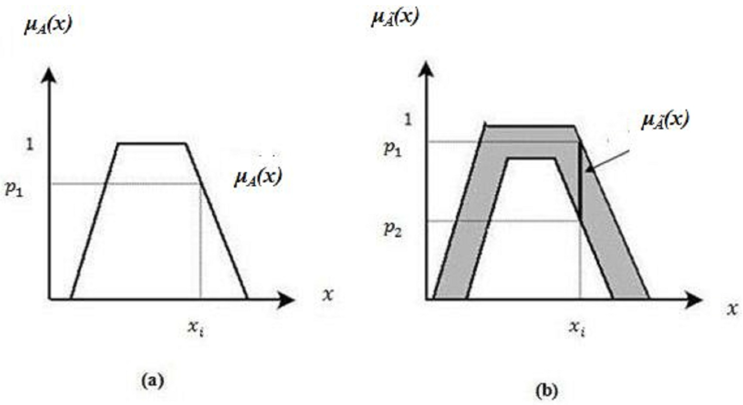
Let us define A as a T1FS and as an IT2FS respectively as shown in Figure 1a,b. For a specific value of x, say , we get a single membership value in A. However, for the same value of , there is a set of interval membership values between and in .
Two key matters are generally addressed in SPP with IT2FSs or T2FS. One is how to find the addition of two arcs to determine the path length and the other is how to compare between the path lengths of two different paths. A variety of methods for addition operation between IT2FSs have been proposed in the literature [52,53,54]. In [52], the authors have used trapezoidal fuzzy set for upper membership function (UMF) and non normal triangular set (the height is less than or equal to 1) for lower membership function (LMF). The canonical forms for such kind of trapezoidal IT2FSs are used in their work [52]. Let = = , where and are respectively as given below.
Similarly = = .
An addition operation on such type of IT2FSs and is defined in [52] as follows.
V. Anusuya and R. Sathya [55] have proposed an algorithm for SPP from a source node to a destination node on a network in which a type-2 fuzzy number is assigned to each arc as its arc length. All the possible paths between source node and destination node and their corresponding path lengths are computed in their proposed algorithm. For this purpose, the authors have added type-2 fuzzy numbers corresponding to the arcs present in the path. Then, they have converted the type-2 fuzzy number representing a path length to its complement form and computed its rank. The path corresponding to the lowest rank has been assigned as the shortest path. Though the authors have claimed that this method is flexible and intelligent, they did not provide any justification for using the complement of type-2 fuzzy number. In [56], the authors assigned a discrete type 2 fuzzy number to each arc of the network and computed the path lengths of all possible paths between source node and destination node using the same method as in [55]. For comparison purpose they have used a function to find the minimum of two discrete type 2 fuzzy numbers representing two paths based on which a metric called similarity measure is computed. The shortest path corresponds to the highest similarity degree.
The motivation behind the work in this article is to find an algorithm for SPP which will be simple enough and effective in real world scenarios. We propose an algorithm to find a shortest path based on Dijkstra’s algorithm in a fuzzy graph, where the arc lengths are trapezoidal IT2FSs. Triangular IT2FS is a special case of trapezoidal IT2FS. Based on the concept described in [53], we derive an operation for adding 2 number of IT2FSs corresponding to the arcs (arc lengths) present in the path. The operator for comparing two IT2FSs can be defined in a wide variety of ways [45,57]. We use centroid based ranking [57] to choose the shortest path associated with the lowest value of centroid.
The paper is organized as follows. Section 2 briefly reviews some basic concepts and definitions on fuzzy graph, type-2 fuzzy set (T2FS), IT2FS, centroid based ranking on IT2FS and path algebra. In Section 3, we describe the proposed algorithm for IT2FSPP where uncertainty associated with IT2FS has been incorporated in Dijkstra’s algorithm. The corresponding path algebra and its generalized algorithm are also presented in this section. We present numerical examples in Section 4 to illustrate the effectiveness of the algorithm. Finally, we conclude in Section 5.
2. Preliminaries
In this section, we introduce fuzzy graph, T2FS, IT2FS, footprint of uncertainty, addition of IT2FSs, centroid based ranking on IT2FS and path algebra to facilitate future discussion.
Definition 1.
Let V be a finite and non empty set. A fuzzy graph is a pair of functions G = , where σ is a fuzzy subset of V and μ is a symmetric fuzzy relation on σ, i.e., σ: and μ: V such that
Definition 2.
[34] A type-2 fuzzy set, denoted as , is characterized by a type-2 membership function , where x ∈ X and u ∈ ⊆ , i.e.,
in which 0 ≤ ≤ 1. Here, x, , u and are respectively primary variable, primary membership function of x, secondary variable and secondary membership function at x. can also be expressed as
Here, and denotes union over all admissible x and u. For discrete universes of discourse ∫ is replaced by ∑.
Definition 3.
Let V be a finite and non empty set. A fuzzy graph is a pair of functions G = , where σ is a fuzzy subset of V and μ is a symmetric fuzzy relation on σ, i.e., σ: and μ: V such that
Definition 4.
[34] IT2FS is a special case of T2FS which has uniform shading over the entire FOU. A T2FS with uniform secondary membership function is called an IT2FS. Let be an IT2FS, then it is described as
Here, x is the primary variable, , an interval in [0,1], is the primary membership of x, u is the secondary variable and is the secondary membership function at x.
A trapezoidal IT2FS is shown in Figure 2. The reference points and their corresponding heights of the upper and the lower membership functions of IT2FS characterize an IT2FS. The shaded region is the FOU. It is bounded by an upper membership function (UMF), denoted by or , and a lower membership function (LMF), denoted by or . The UMF and LMF both are type-1 fuzzy Sets (T1FSs).
Let us consider two trapezoidal IT2FSs and , where
The addition [53] operation (⊕) between the two trapezoidal IT2FSs and is defined in (6) as follows:
It shows that the result of addition operation is also a trapezoidal IT2FS. So, it can also be added to another IT2FS , the result of which is again an IT2FS, say . In this way, we can add n number of IT2FSs as defined below in (7).
Here, (7) represents an IT2FS. So, we can conclude that the path between two nodes can be represented by an IT2FS, obtained by adding all the IT2FSs corresponding to the arcs, present in the path.
Definition 5.
The path between any two nodes in a fuzzy graph can be represented by an IT2FS, obtained by adding all the IT2FSs corresponding to the arcs present in the path.
As an example, let us consider a fuzzy graph, shown in Figure 3, having 6 nodes and 9 arcs. The arcs are represented by IT2FSs, which are shown in Table 1. Let is an IT2FS, where i and j denote two nodes associated with the arc () directly. Using the law of association on addition operation of IT2FSs, explained above, the path from the node 1 to the node 6, through the nodes 2, 3 and 5 can be expressed as follows:
Here, and are two IT2FSs representing two paths, first one from the node 1 to node 3 through the node 2 and the other one from the node 1 to the node 5 through the nodes 2 and 3. Note that there are two different paths represented by and , from node 1 to node 3. represents the direct connection by the arc (1,3) and is through the node 2.
Ranking of IT2FSs is important for IT2FSPP. Since IT2FSs do not form any natural linear order, like real numbers, a key issue is how to compare two IT2FSs. Defuzzification, in general, is a method to map an IT2FS into a real number. The real numbers are then compared. Many defuzzification [57,58,59,60,61] methods are present in the literature. In this study, the centroid based ranking method [61] is used to solve the IT2FSPP.
Definition 6.
[61] The centroid of an IT2FS is the union of the centroids of all its embedded T1FSs , which is a closed interval as follows in (8).
Here, and are respectively the minimum and maximum of all centroids of the embedded T1FSs in the FOU of as given below in (9) and (10).
Equations (9) and (10) can be computed [61,62,63] from the lower and upper membership functions of as follows:
Here is the switch point that marks the change from to and is the switch point that marks the change from to . N is the number of discrete points based on which the domain of x for has been discretized. Let < < ... < , where and are respectively the smallest and highest discrete values of x. The pseudocode for computing L and are given in Algorithm 1 [61,62,63]. Here, we have considered the discrete version of the algorithm.
Similarly, R and can be computed. Then, the average of and of IT2FS , i.e., is computed using (16), which is the centroid based ranking value of IT2FS .
The larger is the centroid value , the greater is the arc length of the corresponding IT2FS . As an example, let us consider the IT2FS = , used for the arc (1,2), as shown in Table 1. To find the centroid based rank of , we consider N, specified in Algorithm 1, as 50. We compute an initial point = 7.86 using (13). This value is assigned in . Then the value of k = 21 is computed following the loop defined in step 4. From (15), we get = 7.28 using the value of k as 21. As the values of (=7.86) and (=7.28) are not equal, we repeat the do — while loop (step 2 to step 13) of Algorithm 1 until the value of and converges, i.e., they have the same value, which is 7.24 for this example. So, we get the value of = 7.24. Similarly, we compute the value of = 8.56. The average of and of IT2FS , i.e., = 7.90 is computed using (16).
| Algorithm 1 Pseudocode for computing left switch point L and . | |
| 1: | Initialize |
| where
| |
| 2: | do |
| 3: | Set = |
| 4: | Find k (1 ≤k ≤ ) such that ≤ ≤ |
| 5: | for i=1 to N do |
| 6: | if then |
| 7: | = |
| 8: | else |
| 9: | = |
| 10: | end if |
| 11: | end for |
| 12: | Compute |
| 13: | while ( is not equal to ) |
| 14: | = (= ) and L=k |
| 15: | Print the value of and L and terminate |
Definition 7.
Let and are two IT2FSs. Then
- ≻ if and only if > .
- ≺ if and only if < .
- ∼ if and only if = .
As an example, let us consider a fuzzy graph, shown in Figure 3. Here, node 1 is connected with node 2 and node 3. The arcs (1,2) and (1,3) are represented by IT2FSs, which are shown in Table 1. By the centroid based ranking value, we get = 7.90 and = 8.12, i.e., ≺ . Thus, the length of the arc represented by is less than the length of the arc represented by .
Path Algebra
Here, we consider the SPP in an algebraic framework, namely path algebra for the purpose of generalization of the proposed algorithm.
Definition 8.
Let E be a set and ⊕ be an operator on E and ϵ ∈ E. Then is said to be a monod with zero element ϵ if
- (i)
- ⊕ is associative: ∀ a, b, c ∈ E, a ⊕ (b ⊕ c) = (a ⊕ b) ⊕ c
- (ii)
- ∀ a ∈ E, a ⊕ ϵ = ϵ ⊕ a = a.
A monod is said to be commutative if ⊕ is commutative: ∀ a, b ∈ E, a ⊕ b = b ⊕ a.
Definition 9.
[64] Let us consider an algebraic structure consisting of a set E, with two internal operator ⊕ (“addition”) and ⊗ (“multiplication”). is a semiring if the following properties hold:
- (i)
- is a commutative monod with zero element ϵ.
- (ii)
- is a monod with unit element e.
- (iii)
- ⊗ is a right and left distributive with respect to ⊕.
- (iv)
- ϵ is absorbing, i.e., ϵ ⊗ a = a ⊗ ϵ = ϵ ()
Definition 10.
[64] being a monod, the binary relation ≤ on E is defined as: a ≤ b if ∃ c ∈ E such that b = a ⊕ c, is a preorder relation (transitive and reflexive) called the canonical preorder. A monod is known as canonically ordered if the canonical preorder is an order, or equivalently if ≤ is antisymmetric relation, i.e., (a ≤ b and b ≤ a ⇒ a = b). A semiring in which is canonically ordered is a diod.
Definition 11.
[65] A path algebra is an algebraic structure with the following two properties.
- 1.
- is a diod.
- 2.
- The operator ⊕ is idempotent, i.e., ∀ a ∈ L, a ⊕ a = a.
The second property imposes a natural order in the path algebra.
3. Proposed Dijkstra’s Algorithm for IT2FSPP
Proposed algorithm is the extension of Dijkstra’s algorithm for SPP. We have incorporated the concept of uncertainty in Dijkstra’s algorithm using IT2FS as an arc length. The pseudocode of the proposed Dijkstra’s algorithm for IT2FSPP is shown in Algorithm 2. The proposed algorithm finds the shortest path from a source node to a destination node of a directed acyclic graph. The source and destination nodes are different and denoted respectively by s and d. Q is used to store all the nodes of the fuzzy graph G, which are currently unvisited. Let v be a node of fuzzy graph G, then is the current shortest distance of v from the source node and is the length of the arc connecting two adjacent nodes u and v. The and both are expressed by IT2FS and stores the node, previous to the current node v along the shortest path from the source node. We use a function that receives an IT2FS as input and returns the centroid based ranking value, i.e., rank of the IT2FS. Another variable is used to store the rank of the shortest path from the source node to v. u is used as a node in Q which has currently the lowest value of rank.
In this study, we are interested only for the shortest path from node s to node d. So, we do not need to check whether Q is empty or not as done in original Dijkstra’s algorithm. Once we get the destination node d, we terminate the algorithm. Finally, gives the length of the shortest path from s to d, which is an IT2FS. We can also find the corresponding path starting from the destination node and moving backward to the source node using .
The classical Dijkstra’s algorithm has time complexity of when adjacency matrix is used. Here, represents the number of nodes in the graph. In our proposed algorithm, we have used the well known KM algorithm [57,61,66], for computing the centroid based ranking value of an IT2FS, as described earlier in Definition 6. The time complexity to compute the rank of an IT2FS, which represents a path is , where N is the number of discretization points in the interval and M is the number of iterations required for convergence. Hence, the computational complexity of the proposed algorithm is .
| Algorithm 2 Pseudocode of the proposed algorithm. | ||
| 1: | rank[s] ← 0 | |
| 2: | dist[s] ← null | ▷ Corresponding IT2FS is empty |
| 3: | add s to Q | |
| 4: | for each vertex i (except the s) in the fuzzy graph do | |
| 5: | rank[i] ← INFINITY | |
| 6: | add i to Q | ▷ Initialize Q with all the nodes of the graph |
| 7: | end for | |
| 8: | ||
| 9: | while (u is not the the destination node d) do | ▷ Shortest path from s to d |
| 10: | remove the node u from Q | |
| 11: | for every node v adjacent to u do | |
| 12: | temp_dist ← dist ⊕ arc_length() | ▷ as described in (6) |
| 13: | temp_rank ← centroid_rank (temp_dist) | |
| 14: | if (temp_rank < rank[v]) then | |
| 15: | dist ← temp_dist | |
| 16: | rank[v] ← temp_rank[v] | |
| 17: | previous[v]←u | |
| 18: | end if | |
| 19: | end for | |
| 20: | vertex in Q with the smallest rank value | |
| 21: | end while | |
| 22: | The IT2FS is an IT2FS and it represents length of the shortest path. | |
In the path algebra L, defined in Definition 11, let p be the set of all IT2FSs and the binary operators ⊕ and ⊗ are replaced respectively by among two IT2FSs for which the rank is less and addition of two IT2FSs. This two operators are defined below.
, a ⊕ b = where
=
Here, is the centroid based ranking value of a and the operator is same as the addition operation of two IT2FSs, respectively defined in (13) and (6). Then the algebraic structure L = follows the properties of path algebra which corresponds to the generalization of the proposed algorithm, i.e., Dijkstra’s algorithm using IT2FSs, where, zero element and unit element e = ((0, 0, 0, 0; 1, 1), (0, 0, 0, 0; 1, 1)). Here, ϵ is the largest IT2FS, i.e., = ∞. The proof that the proposed algebraic framework is a path algebra is provided in Appendix A. The path algebra has been widely applied for the formulation of graph path finding problems [64,67].
The generalized algorithm for the proposed modification based on path algebra L = is presented in Algorithm 3. Here, is the current shortest path length from the source node s to a node l of the fuzzy graph G. The weights of the edges in G, i.e., arc lengths are the IT2FSs and G does not contain any cycle of negative length. is the set of all nodes connected to u by an arc. From Gondran’s theorem [68,69] we can claim that the generalized algorithm for the proposed modification of Dijkstra’s algorithm always converges.
From the generalized algorithm, we can also compute its time complexity. In the worst case, outer loop (while-do) is executed times and the inner loop is executed times because for a particular node the maximum possible numbers of its neighbors is . Hence, the time complexity of the algorithm is . It is worth mentioning that for computation of time complexity of Algorithm 3, step 10 has been considered as a single unit. The operations and , used in step 10, have not been considered separately for the execution of step 10.
| Algorithm 3 Pseudocode of the generalized algorithm for the proposed modification. | ||
| 1: | ← e | |
| 2: | add s to Q | |
| 3: | for each vertex i (except s) in G do | |
| 4: | ← ϵ | ▷ϵ is the highest IT2FS. |
| 5: | add i to Q | |
| 6: | end for | |
| 7: | s | |
| 8: | while (u is not the destination node d) do | |
| 9: | for all v ∈ { ∩ Q} do | ▷ is the set of all nodes connected to u through an arc. |
| 10: | ← (, (, arc_length)) | ▷ Choose a node v for which is minimum. |
| 11: | end for | |
| 12: | previous[v]←u | |
| 13: | Q ← Q \ {u} | |
| 14: | Find u, u ∈ Q such that is minimum among all s, i ∈ Q. | ▷ Using the natural order in the monod |
| 15: | end while | |
| 16: | gives the shortest path length from s to d. | |
4. Numerical Examples
We have used two example graphs, shown in Figure 3 and Figure 4, to illustrate the proposed algorithm.
4.1. Example 1
We demonstrate our algorithm step by step by an example graph [5,16], shown in Figure 3. Let us consider the source node is 1 and the destination node is 6. IT2FSs corresponding to the arcs of the graph are shown in Table 1. We have collected the values of IT2FSs from [57] and assigned them to the arcs of the graph randomly. We have to find the shortest path between the nodes 1 and 6. The steps of the algorithm and the corresponding outputs/results are shown in Table 2. In Table 2, S contains the nodes, already processed and Q contains the nodes not yet visited.
4.2. Example 2
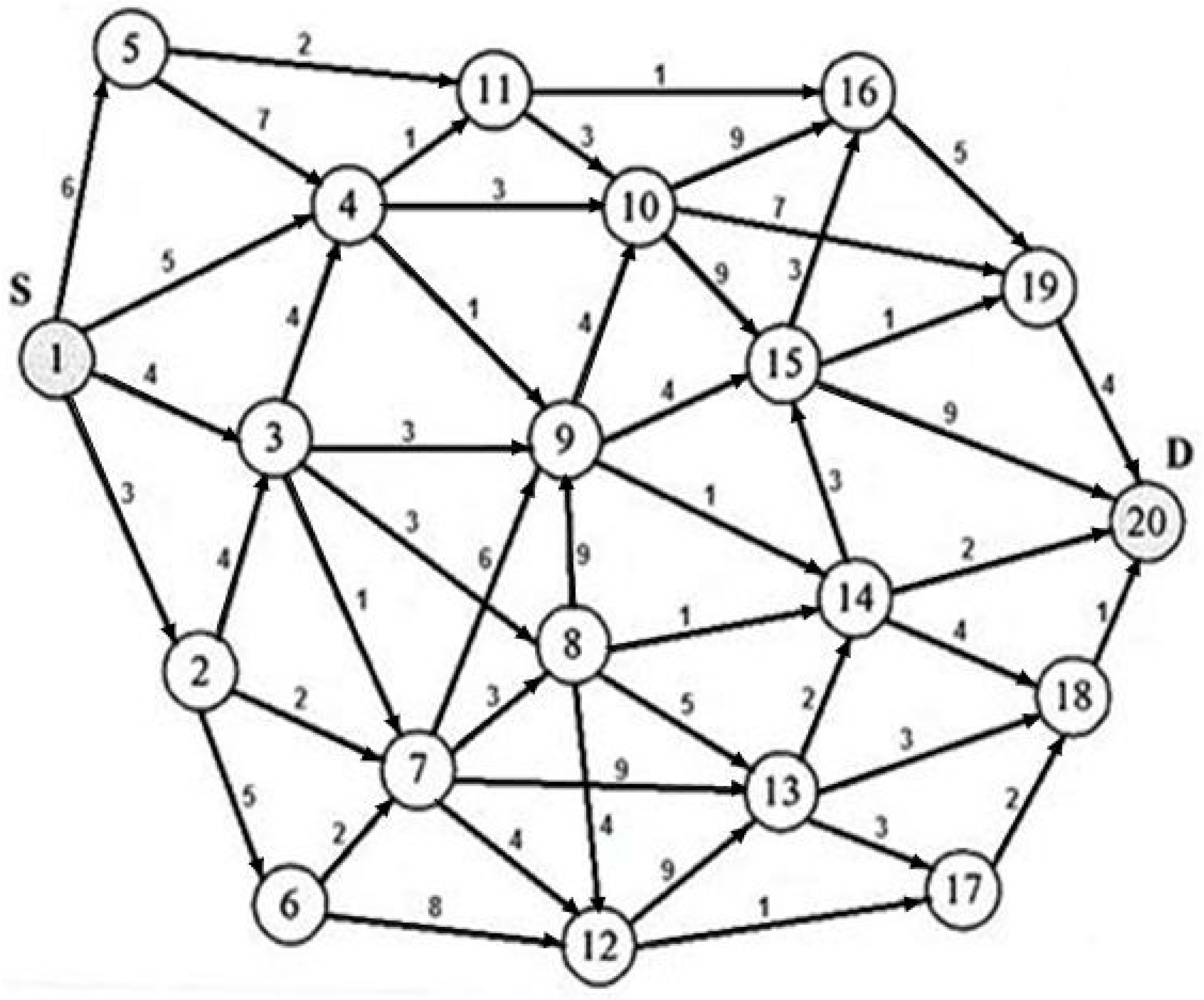
We have tested our algorithm on a graph [5], shown in Figure 4, with 20 nodes and 49 edges. Nodes are numbered arbitrarily from 1 to 20. Let the source node is 1 and the destination node is 20. The arc lengths of the graph are shown in Table 3 in the form of trapezoidal IT2FSs. For this graph, we have taken nine IT2FSs from [57], which are indexed from one to nine as shown in Table 3 and assigned to the arcs of the graph. Each arc is annotated with the corresponding index value. The shortest path from source node 1 to destination node 20, we have obtained is and the corresponding shortest path length is 2.209, which is the rank value of the destination node 20. The corresponding table for the explanation its steps is not provided for its large space.
There exists two algorithms proposed in [55,56] for SPP with T2FSs, already mentioned in the section of introduction. In the both the algorithms, firstly all the possible paths between source and destination nodes are computed. However, the problem of finding all possible paths between two nodes in a graph is NP hard. The time complexity of the proposed algorithm, i.e., represents the worst possible situation when all the nodes of the graph are to be visited to reach the destination node d. In general, for a single destination node for FSPP, all the nodes of the graph may not be required to be visited in most of the cases. So, the actual time required for the proposed algorithm is much less than . As an example, let us consider the graph, shown in Figure 3, where node 6 has been used as destination node. To find the corresponding path (from node 1 to node 6), all the nodes of the graph have been visited, already explained in Table 2. If we consider, say node 4 in place of 6 as the destination node, the algorithm will determine after step 4 of Table 2 and node 6 is not required to visit and process. Thus, the time to find the path from source node to node 4 is much less than that for the path to node 6.
5. Conclusions
In this work, we investigate the FSPP, where arc costs are represented by IT2FSs. The significance of using IT2FSs in SPP is described in this paper. We modify the classical Dijkstra’s algorithm by incorporating the uncertainty using IT2FS for SPP from a single source to a single destination. Numerical examples are used to illustrate the effectiveness of the proposed algorithm. The main contribution of this study is to provide an algorithmic approach for SPP in uncertain environment using IT2FSs as arc lengths. The proposed algorithm is simple enough and effective for real world scenarios. We also study the path algebra and the corresponding generalized algorithm of the FSPP. In future, the proposed method can be applied to real world problems in transportation, supply chain management and other relevant fields.
Acknowledgments
The authors sincerely thank all the referee(s) for their valuable suggestions and comments, which were very much useful to improve the paper significantly.
Author Contributions
All of the authors provided equal contributions to the paper.
Conflicts of Interest
The authors declare no conflict of interest.
Appendix A
In order to prove that L = is a path algebra corresponding to the proposed algorithm for a IT2FSPP, first we prove L as diod and then the operator as idempotent. The path algebra L needs to hold following 5 properties (P1–P5) to be a diod. First four properties (P1–P4) are required for L to be a semiring, defined in Definition 9. The fifth property (P5) is to make the semiring a diod as defined in Definition 10. Finally, a diod needs to follow the sixth property (P6), i.e., if the operator of the diod L is idempotent then L is a path algebra.
P1. is a commutative monod with unit element ϵ if the following three properties hold.
- (1)
- ∀ a, b, c ∈ p, ( (a, b), c) = ( (, ), ), i.e., operator is associate.Proof: As is the centroid based ranking value of a and ranking value is always a real number. So, ( (a, b), c) = (, , )Thus = (, , )It proves operator is associate.
- (2)
- ∈ p, (a, ϵ) = min(ϵ, a) = a.Proof: =ϵ being the largest IT2FS, = ∞.= aFor the same reason = a.
- (3)
- The centroid based ranking value of IT2FSs are non negative real numbers. So,∀ a,b ∈ p, (a, b) = (, ) = = .It proves that is commutative monod.
P2. is a monod with unit element e if the following two properties hold.
- (1)
- ∀ a, b, c ∈ p, ((a,b), c) = (a, b, c) defined in (6).Now, (a, (b,c)) =It proves that operator is associate.
- (2)
- Let . As e = (( 0, 0, 0, 0; 1, 1 ), ( 0, 0, 0, 0; 1, 1)), following the addition operation defined in (6).Similarly, = a.It proves that ∀ a ∈ p, (a e) = (e, a) = a.
P3.
So, (A2) and (A3) return the same value. Similarly, we can show that
( (b, c), a) = ( (a, b), (a, c)).
It proves that is a right and left distributive with respect to .
P4.
- Let .
- As , following the addition operation defined in (6), we can get ∀a ∈ p, (ϵ, a) = (a ,ϵ) = ϵ. It proves that ϵ is absorbing.
The algebraic structure L = holds all of the above the four properties (P1–P4) of semiring.
P5.
- The monod is canonically ordered as the binary relation ≤ on p is antisymmetric relation, i.e., ≤ and ≤ ⇒ = . So, a and b are equal. So, the monod is canonically ordered. A semiring such that is canonically ordered is called a diod. So, L is a diod.
P6.
- The operator is idempotent because ∀ a ∈ p, (a, a) = (, ) = a.
L follows all the properties of path algebra. So, it is proved that L is a path algebra.
References
- Dijkstra, E.W. A note on two problems in connexion with graphs. Numer. Math. 1959, 1, 269–271. [Google Scholar] [CrossRef]
- Cormen, T.H.; Leiserson, C.E.; Rivest, R.L.; Stein, C. Introduction to Algorithms, 2nd ed.; The MIT Press: Cambridge, MA, USA, 2001. [Google Scholar]
- Dubois, D.; Parde, H. Fuzzy Sets and Systems: Theory and Applications; Academic Press: NewYork, NY, USA, 1980; Volume 144. [Google Scholar]
- Klein, C.M. Fuzzy shortest paths. Fuzzy Sets Syst. 1991, 39, 27–41. [Google Scholar] [CrossRef]
- Hassanzadeh, R.; Mahdavi, I.; Mahdavi-Amiri, N.; Tajdin, A. A genetic algorithm for solving fuzzy shortest path problems with mixed fuzzy arc lengths. Math. Comput. Model. 2013, 57, 84–99. [Google Scholar] [CrossRef]
- Chanas, S.; Kamburowski, J. The Fuzzy Shortest Route Problem. In Interval and Fuzzy Mathematics; Proceeding Polish Symposium; Technical University of Poznan: Poznan, Poland, 1983; pp. 35–41. [Google Scholar]
- Blue, M.; Bush, B.; Puckett, J. Unified approach to fuzzy graph problems. Fuzzy Sets Syst. 2002, 125, 355–368. [Google Scholar] [CrossRef]
- Okada, S. Fuzzy shortest path problems incorporating interactivity among paths. Fuzzy Sets Syst. 2004, 142, 335–357. [Google Scholar] [CrossRef]
- Takahashi, M.; Yamakami, A. On Fuzzy Shortest Path Problems with Fuzzy Parameters: An Algorithmic Approach. In Proceedings of the Annual Meeting of the North American Fuzzy Information Processing Society, NAFIPS 2005, Detroit, MI, USA, 26–28 June 2005; pp. 654–657.
- Mahdavi, I.; Nourifar, R.; Heidarzade, A.; Amiri, N.M. A dynamic programming approach for finding shortest chains in a fuzzy network. Appl. Soft Comput. 2009, 9, 503–511. [Google Scholar] [CrossRef]
- Yager, R.R. Paths of least resistance in possibilistic production systems. Fuzzy Sets Syst. 1986, 19, 121–132. [Google Scholar] [CrossRef]
- Lin, K.C.; Chern, M.S. The fuzzy shortest path problem and its most vital arcs. Fuzzy Sets Syst. 1993, 58, 343–353. [Google Scholar] [CrossRef]
- Okada, S.; Soper, T. A shortest path problem on a network with fuzzy arc lengths. Fuzzy Sets Syst. 2000, 109, 129–140. [Google Scholar] [CrossRef]
- Nayeem, S.M.A.; Pal, M. Shortest path problem on a network with imprecise edge weight. Fuzzy Optim. Decis. Mak. 2005, 4, 293–312. [Google Scholar] [CrossRef]
- Moazeni, S. Fuzzy shortest path problem with finite fuzzy quantities. Appl. Math. Comput. 2006, 183, 160–169. [Google Scholar] [CrossRef]
- Hernandes, F.; Lamata, M.T.; Verdegay, J.L.; Yamakami, A. The shortest path problem on networks with fuzzy parameters. Fuzzy Sets Syst. 2007, 158, 1561–1570. [Google Scholar] [CrossRef]
- Deng, Y.; Chen, Y.; Zhang, Y.; Mahadevan, S. Fuzzy Dijkstra algorithm for shortest path problem under uncertain environment. Appl. Soft Comput. 2012, 12, 1231–1237. [Google Scholar] [CrossRef]
- Hansen, P. Bicriterion Path Problems. In Multiple Criteria Decision Making Theory and Application; Springer: Berlin/Heidelberg, Germany, 1980; pp. 109–127. [Google Scholar]
- Sengupta, A.; Pal, T.K. On comparing interval numbers. Eur. J. Operat. Res. 2000, 127, 28–43. [Google Scholar] [CrossRef]
- Min, F.; Xu, J. Semi-greedy heuristics for feature selection with test cost constraints. Granul. Comput. 2016, 1, 199–211. [Google Scholar] [CrossRef]
- Maciel, L.; Ballini, R.; Gomide, F. Evolving granular analytics for interval time series forecasting. Granul. Comput. 2016. [Google Scholar] [CrossRef]
- Song, M.; Wang, Y. A study of granular computing in the agenda of growth of artificial neural networks. Granul. Comput. 2016. [Google Scholar] [CrossRef]
- Liu, H.; Gegov, A.; Cocea, M. Rule-based systems: A granular computing perspective. Granul. Comput. 2016. [Google Scholar] [CrossRef] [Green Version]
- Lingras, P.; Haider, F.; Triff, M. Granular meta-clustering based on hierarchical, network, and temporal connections. Granul. Comput. 2016, 1, 71–92. [Google Scholar] [CrossRef]
- Skowron, A.; Jankowski, A.; Dutta, S. Interactive granular computing. Granul. Comput. 2016, 1, 95–113. [Google Scholar] [CrossRef]
- Dubois, D.; Prade, H. Bridging gaps between several forms of granular computing. Granul. Comput. 2016, 1, 115–126. [Google Scholar] [CrossRef]
- Apolloni, B.; Bassis, S.; Rota, J.; Galliani, G.L.; Gioia, M.; Ferrari, L. A neurofuzzy algorithm for learning from complex granules. Granul. Comput. 2016. [Google Scholar] [CrossRef]
- Mendel, J.M.; John, R.I.B. Type-2 fuzzy sets made simple. IEEE Trans. Fuzzy Syst. 2002, 10, 117–127. [Google Scholar] [CrossRef]
- Zadeh, L.A. The concept of a linguistic variable and its application to approximate reasoning-I. Inform. Sci. 1975, 8, 199–249. [Google Scholar] [CrossRef]
- Dereli, T.; Altun, K. Technology evaluation through the use of interval type-2 fuzzy sets and systems. Comput. Ind. Eng. 2013, 65, 624–633. [Google Scholar] [CrossRef]
- Chen, S.M.; Yang, M.W.; Yang, S.W.; Sheu, T.W.; Liau, C.J. Multicriteria fuzzy decision making based on interval-valued intuitionistic fuzzy sets. Expert Syst. Appl. 2012, 39, 12085–12091. [Google Scholar] [CrossRef]
- Wang, W.; Liu, X.; Qin, Y. Multi-attribute group decision making models under interval type-2 fuzzy environment. Knowl.-Based Syst. 2012, 30, 121–128. [Google Scholar] [CrossRef]
- Chen, T.Y. A linear assignment method for multiple-criteria decision analysis with interval type-2 fuzzy sets. Appl. Soft Comput. 2013, 13, 2735–2748. [Google Scholar] [CrossRef]
- Mendel, J.M.; John, R.I.; Liu, F. Interval type-2 fuzzy logic systems made simple. IEEE Trans. Fuzzy Syst. 2006, 14, 808–821. [Google Scholar] [CrossRef]
- Mendel, J.M. A comparison of three approaches for estimating (synthesizing) an interval type-2 fuzzy set model of a linguistic term for computing with words. Granul. Comput. 2016, 1, 59–69. [Google Scholar] [CrossRef]
- Wilke, G.; Portmann, E. Granular computing as a basis of human–data interaction: A cognitive cities use case. Granul. Comput. 2016, 1, 181–197. [Google Scholar] [CrossRef]
- Loia, V.; D’Aniello, G.; Gaeta, A.; Orciuoli, F. Enforcing situation awareness with granular computing: A systematic overview and new perspectives. Granul. Comput. 2016, 1, 127–143. [Google Scholar] [CrossRef]
- Yao, Y. A triarchic theory of granular computing. Granul. Comput. 2016, 1, 145–157. [Google Scholar] [CrossRef]
- Ciucci, D. Orthopairs and granular computing. Granul. Comput. 2016, 1, 159–170. [Google Scholar] [CrossRef]
- Kreinovich, V. Solving equations (and systems of equations) under uncertainty: How different practical problems lead to different mathematical and computational formulations. Granul. Comput. 2016, 1, 171–179. [Google Scholar] [CrossRef]
- Ciesa, M.; Grigolato, S.; Cavalli, R. Analysis on vehicle and walking speeds of search and rescue ground crews in mountainous areas. J. Outdoor Recreat. Tour. 2014, 5, 48–57. [Google Scholar] [CrossRef]
- Chiou, C.R.; Tsai, W.L.; Leung, Y.F. A GIS-dynamic segmentation approach to planning travel routes on forest trail networks in Central Taiwan. Landsc. Urban Plan. 2010, 97, 221–228. [Google Scholar] [CrossRef]
- Livi, L.; Sadeghian, A. Granular computing, computational intelligence, and the analysis of non-geometric input spaces. Granul. Comput. 2016, 1, 13–20. [Google Scholar] [CrossRef]
- Peters, G.; Weber, R. DCC: A framework for dynamic granular clustering. Granul. Comput. 2016, 1, 1–11. [Google Scholar] [CrossRef]
- Wu, D.; Mendel, J.M. Computing with words for hierarchical decision making applied to evaluating a weapon system. IEEE Trans. Fuzzy Syst. 2010, 18, 441–460. [Google Scholar] [CrossRef]
- Zadeh, L.A. Fuzzy logic = computing with words. IEEE Trans. Fuzzy Syst. 1996, 4, 103–111. [Google Scholar] [CrossRef]
- Wang, J.H.; Hao, J. A new version of 2-tuple fuzzy linguistic representation model for computing with words. IEEE Trans. Fuzzy Syst. 2006, 14, 435–445. [Google Scholar] [CrossRef]
- Herrera, F.; Alonso, S.; Chiclana, F.; Herrera-Viedma, E. Computing with words in decision making: Foundations, trends and prospects. Fuzzy Optim. Decis. Mak. 2009, 8, 337–364. [Google Scholar] [CrossRef]
- Yager, R.R. On the retranslation process in Zadeh’s paradigm of computing with words. IEEE Trans. Syst. Man Cybern. B Cybern. 2004, 34, 1184–1195. [Google Scholar] [CrossRef] [PubMed]
- Xu, Z.; Wang, H. Managing multi-granularity linguistic information in qualitative group decision making: An overview. Granul. Comput. 2016, 1, 21–35. [Google Scholar] [CrossRef]
- Antonelli, M.; Ducange, P.; Lazzerini, B.; Marcelloni, F. Multi-objective evolutionary design of granular rule-based classifiers. Granul. Comput. 2016, 1, 37–58. [Google Scholar] [CrossRef]
- Chiao, K.P. Trapezoidal Interval Type-2 Fuzzy Set Extension of Analytic Hierarchy Process. In Proceedings of the 2012 IEEE International Conference on Fuzzy Systems (FUZZ-IEEE), Brisbane, Australia, 10-15 June 2012; pp. 1–8.
- Lee, L.W.; Chen, S.M. A New Method for Fuzzy Multiple Attributes Group Decision-Making Based on the Arithmetic Operations of Interval Type-2 Fuzzy Sets. In Proceedings of the 2008 International Conference on Machine Learning and Cybernetics, Kunming, China, 12–15 July 2008; Volume 6, pp. 3084–3089.
- Qin, J.; Liu, X. Frank aggregation operators for triangular interval type-2 fuzzy set and its application in multiple attribute group decision making. J. Appl. Math. 2014, 2014, 923213. [Google Scholar] [CrossRef]
- Anusuya, V.; Sathyaa, R. Shortest path with complement of type-2 fuzzy number. Malaya J. Mat. 2013, 1, 71–76. [Google Scholar]
- Anusuya, V.; Sathyaa, R. Type-2 fuzzy shortest path on similarity measure. Bull. Math. Stat. Res. 2014, 2, 418–422. [Google Scholar]
- Wu, D.; Mendel, J.M. A comparative study of ranking methods, similarity measures and uncertainty measures for interval type-2 fuzzy sets. Inform. Sci. 2009, 179, 1169–1192. [Google Scholar] [CrossRef]
- Zimmermann, H.J. Fuzzy Control. In Fuzzy Set Theory—And Its Applications; Springer: Dordrecht, The Netherlands, 1996; pp. 203–240. [Google Scholar]
- Fortemps, P.; Roubens, M. Ranking and defuzzification methods based on area compensation. Fuzzy Sets Syst. 1996, 82, 319–330. [Google Scholar] [CrossRef]
- Van Leekwijck, W.; Kerre, E.E. Defuzzification: Criteria and classification. Fuzzy Sets Syst. 1999, 108, 159–178. [Google Scholar] [CrossRef]
- Karnik, N.N.; Mendel, J.M. Centroid of a type-2 fuzzy set. Inform. Sci. 2001, 132, 195–220. [Google Scholar] [CrossRef]
- Morales, O.S.; Devia, J.H.S.; Mendez, J.J.S. Centroid of an interval type-2 fuzzy set: Continuous vs. discrete. Ingeniería 2011, 16, 67–78. [Google Scholar]
- Wu, D.; Mendel, J.M. Uncertainty measures for interval type-2 fuzzy sets. Inform. Sci. 2007, 177, 5378–5393. [Google Scholar] [CrossRef]
- Gondran, M.; Minoux, M. Dioïds and semirings: Links to fuzzy sets and other applications. Fuzzy Sets Syst. 2007, 158, 1273–1294. [Google Scholar] [CrossRef]
- Stawiaski, J. Optimal Path: Theory and Models for Vessel Segmentation. In Proceedings of the International Symposium on Mathematical Morphology and Its Applications to Signal and Image Processing, Verbania-Intra, Italy, 6–8 July 2011; pp. 417–428.
- Mendel, J.M.; Liu, F. Super-exponential convergence of the Karnik-Mendel algorithms for computing the centroid of an interval type-2 fuzzy set. IEEE Trans. Fuzzy Syst. 2007, 15, 309–320. [Google Scholar] [CrossRef]
- Simas, T.; Rocha, L.M. Distance closures on complex networks. Netw. Sci. 2015, 3, 227–268. [Google Scholar] [CrossRef]
- Gondran, M. Algèbre linéaire et Cheminement dans un Graphe. Rech. Opérationnelle 1975, 9, 77–99. [Google Scholar]
- Gondran, M.; Minoux, M. Graphes et Algorithmes, 3rd ed.; Eyrolles: Paris, France, 1995. [Google Scholar]
Figure 1.
() Crisp grades of membership for type-1 fuzzy sets (T1FS) A; () Fuzzy grades of membership for IT2FS .
Figure 1.
() Crisp grades of membership for type-1 fuzzy sets (T1FS) A; () Fuzzy grades of membership for IT2FS .

Figure 2.
Reference points and their heights to determine a footprint of uncertainty (FOU) of IT2FS , where reference points with heights and determine a trapezoidal UMF and reference points with heights and determine a trapezoidal LMF .
Figure 2.
Reference points and their heights to determine a footprint of uncertainty (FOU) of IT2FS , where reference points with heights and determine a trapezoidal UMF and reference points with heights and determine a trapezoidal LMF .
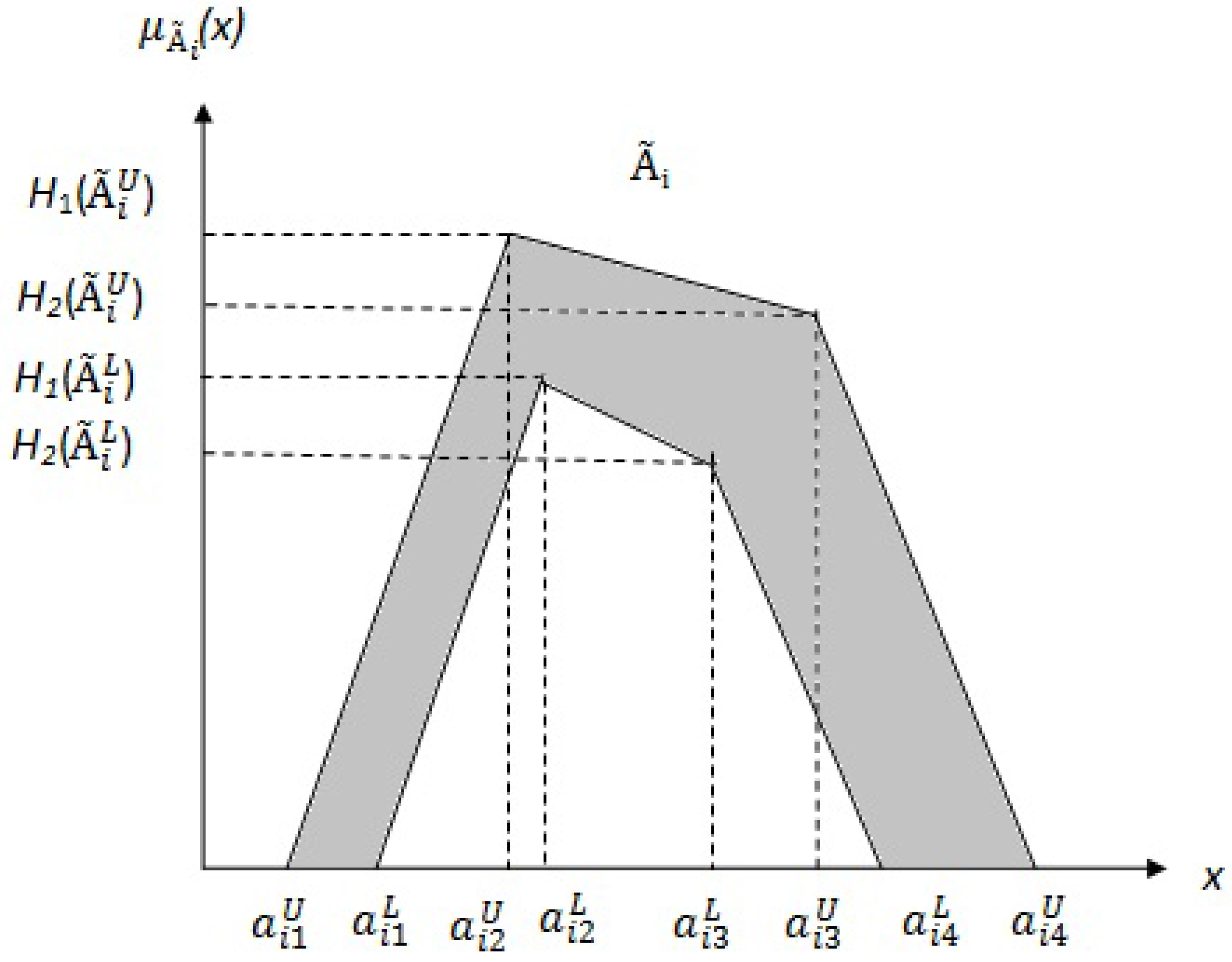
Figure 3.
A classical graph with six nodes and nine edges.
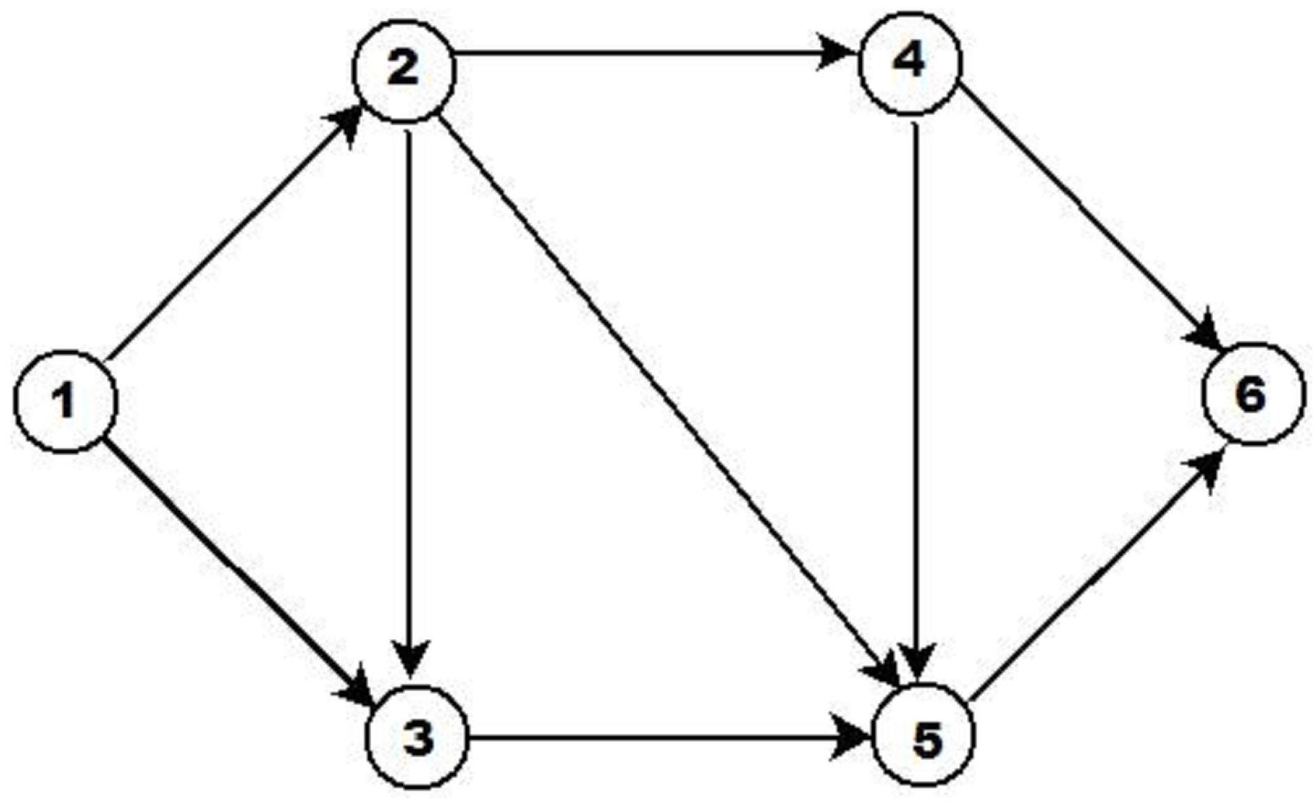
Figure 4.
A graph with 20 nodes and 49 edges.


Table 1.
The arcs of the fuzzy graph, shown in Figure 3.
| Arc | IT2FS Representing an Arc |
|---|---|
| 1–2 | (( 5.38, 7.50, 9.00, 9.81; 1, 1 ), ( 8.29, 8.56, 8.56, 9.21; 0.38, 0.38 )) |
| 1–3 | (( 5.98, 7.75, 8.60, 9.52; 1, 1 ), ( 8.03, 8.36, 8.36, 9.17; 0.57, 0.57 )) |
| 2–3 | (( 7.37, 9.41, 10, 10; 1, 1 ), ( 8.72, 9.91, 10, 10; 1, 1 )) |
| 2–4 | (( 7.37, 9.82, 10, 10; 1, 1 ), ( 9.74, 9.98, 10, 10;1, 1 )) |
| 2–5 | (( 7.37, 9.73, 10, 10; 1, 1 ), ( 9.34, 9.95, 10, 10; 1, 1 )) |
| 3–5 | (( 7.37, 9.59, 10, 10; 1, 1 ), ( 8.95, 9.93, 10, 10;1, 1 )) |
| 4–5 | (( 7.37, 9.73, 10, 10; 1, 1 ), ( 9.34, 9.95, 10, 10; 1, 1 )) |
| 4–6 | (( 7.37, 9.82, 10, 10; 1, 1 ), ( 9.37, 9.95, 10, 10; 1, 1 )) |
| 5–6 | (( 8.68, 9.91, 10, 10; 1, 1 ), ( 9.61, 9.97, 10, 10; 1, 1 )) |
Table 2.
The steps of the proposed algorithm for the graph, shown in Figure 3.
| Step | S | Q |
|---|---|---|
| S = | ||
| = 0.0 | ||
| = ∞ | ||
| = ∞ | ||
| 1 | = ∞ | |
| = ∞ | ||
| = ∞ | ||
| Select the node 1 corresponding to the | ||
| lowest value of rank 0 and remove it from Q. | ||
| S = | ||
| = 0.0 | = 7.90 | |
| Adjacent nodes of 1 = {2,3} | = 8.12 | |
| 2 | = 1 | = ∞ |
| = 1 | = ∞ | |
| = ∞ | ||
| Select the node 2 corresponding to the | ||
| lowest value of rank 7.9 and remove it from Q. | ||
| S = | ||
| = 0.0 | = 8.12 | |
| = 7.9 | = 17.21 | |
| 3 | Adjacent nodes of 2 = {3,4,5} | = 17.46 |
| = 1 | = ∞ | |
| = 1 | Select the node 3 corresponding to the | |
| = 2 | lowest value of rank 8.12 and remove it from Q. | |
| = 2 | ||
| S = | ||
| = 0.0 | = 17.21 | |
| = 7.90 | = 17.46 | |
| = 8.12 | = ∞ | |
| 4 | Adjacent node of 3 = {5} | Select the node 4 corresponding to the |
| = 1 | lowest value of rank 17.21 and remove it from Q. | |
| = 1 | ||
| = 2 | ||
| = 2 | ||
| S = | ||
| = 0.0 | = 17.46 | |
| = 7.90 | = 26.49 | |
| = 8.12 | Select the node 5 corresponding to the | |
| = 17.21 | lowest value of rank 17.46 and remove it from Q. | |
| 5 | Adjacent nodes of 4 = {5,6} | |
| = 1 | ||
| = 1 | ||
| = 2 | ||
| = 2 | ||
| = 4 | ||
| S = | ||
| = 0.0 | = 26.49 | |
| = 7.90 | Select the node 6 which is the destination node. | |
| = 8.12 | ||
| = 17.21 | is the length of the | |
| 6 | = 17.46 | shortest path from source node 1 to destination node 6. |
| Adjacent node of 5 = {6} | ||
| = 1 | = 4, = 2, = 1. | |
| = 1 | So, the shortest path from source node 1 to | |
| = 2 | destination node 6 is | |
| = 2 | ||
| = 4 |
| Index | IT2FSs |
|---|---|
| 1 | ((0, 0, 0.14, 1.97; 1, 1) ( 0, 0, 0.05, 0.66; 1, 1)) |
| 2 | ((0, 0, 0.14, 1.97; 1, 1) ( 0, 0, 0.01, 0.63; 1, 1)) |
| 3 | ((0, 0, 0.26, 2.63; 1, 1) ( 0, 0, 0.05, 0.63; 1, 1)) |
| 4 | ((0, 0, 0.36, 2.63; 1, 1) ( 0, 0, 0.05, 0.63; 1, 1)) |
| 5 | ((0, 0, 0.64, 2.47; 1, 1) ( 0, 0, 0.10, 1.16; 1, 1)) |
| 6 | ((0, 0, 0.64, 2.63; 1, 1) ( 0, 0, 0.09, 0.99; 1, 1)) |
| 7 | ((0.59, 1.50, 2.00, 3.41; 1, 1) ( 0.79, 1.68, 1.68, 2.21; 0.74, 0.74)) |
| 8 | ((0.38, 1.50, 2.50, 4.62; 1, 1) ( 1.09, 1.83, 1.83, 2.21; 0.53, 0.53)) |
| 9 | ((0.09, 1.25, 2.50, 4.62; 1, 1) ( 1.67, 1.92, 1.92, 2.21; 0.30, 0.30)) |
© 2016 by the authors; licensee MDPI, Basel, Switzerland. This article is an open access article distributed under the terms and conditions of the Creative Commons Attribution (CC-BY) license (http://creativecommons.org/licenses/by/4.0/).
Share and Cite
MDPI and ACS Style
Dey, A.; Pal, A.; Pal, T. Interval Type 2 Fuzzy Set in Fuzzy Shortest Path Problem. Mathematics 2016, 4, 62. https://doi.org/10.3390/math4040062
AMA Style
Dey A, Pal A, Pal T. Interval Type 2 Fuzzy Set in Fuzzy Shortest Path Problem. Mathematics. 2016; 4(4):62. https://doi.org/10.3390/math4040062
Chicago/Turabian StyleDey, Arindam, Anita Pal, and Tandra Pal. 2016. "Interval Type 2 Fuzzy Set in Fuzzy Shortest Path Problem" Mathematics 4, no. 4: 62. https://doi.org/10.3390/math4040062
Note that from the first issue of 2016, this journal uses article numbers instead of page numbers. See further details here.