
Certain Concepts of Bipolar Fuzzy Directed Hypergraphs


Department of Mathematics, University of the Punjab, New Campus, Lahore 54590, Pakistan
*
Author to whom correspondence should be addressed.
Mathematics 2017, 5(1), 17; https://doi.org/10.3390/math5010017
Submission received: 15 December 2016
/
Revised: 17 February 2017
/
Accepted: 22 February 2017
/
Published: 4 March 2017
Abstract
:A hypergraph is the most developed tool for modeling various practical problems in different fields, including computer sciences, biological sciences, social networks and psychology. Sometimes, given data in a network model are based on bipolar information rather than one sided. To deal with such types of problems, we use mathematical models that are based on bipolar fuzzy (BF) sets. In this research paper, we introduce the concept of BF directed hypergraphs. We describe certain operations on BF directed hypergraphs, including addition, multiplication, vertex-wise multiplication and structural subtraction. We introduce the concept of -tempered BF directed hypergraphs and investigate some of their properties. We also present an algorithm to compute the minimum arc length of a BF directed hyperpath.
1. Introduction
Graph theory has become a powerful conceptual framework for the modeling and solution of combinatorial problems that arise in various areas, including mathematics, computer science and engineering. Graphs are only useful for modeling of the pairwise communication. However, many times (for example, in statistical physics and effective theories), one works with such interactions that are based on more than two particles. To deal with such kinds of interactions, we use a hyperedge, as it contains more than two vertices. Hypergraphs [1], a generalization of graphs, have many properties that are the basis of different techniques that are used in modern mathematics. Hypergraphs are stated as the extended form of ordinary graphs in the way that they contain a finite collection of points and a set of hyperarcs defined as a subset of vertices. The applicability of graph theory has widened by the generalization of undirected graphs, called undirected hypergraphs, which have been proven to be more useful as mathematical modeling tools. In real-world applications, hypergraph techniques appear very useful in many places, including declustering problems, which are important to increase the performance of parallel databases [2]. Hypergraphs can be demonstrated as a useful engine (or tool) to model concepts and systems in different fields of discrete mathematics. There are different types of hypergraphs that have been broadly utilized in computer science as a suitable mathematical model. There are many complex phenomena and concepts in many areas, including rewriting systems, problem solving, databases and logic programming, which can be represented using hypergraphs [3]. The most used hypergraphs in computer science are undirected hypergraphs [4]. Directed hypergraphs are used to solve and model certain problems arising in deductive databases and in model checking.
There are many complicated phenomena in science and technology in which available information is not accurate. For such types of problems, we use mathematical models that contain elements of uncertainty. These mathematical models are based on fuzzy set theory. The idea of fuzzy sets was given by Zadeh [5]. Fuzzy set theory has many applications in many disciplines, including management sciences, decision theory and robotics. Fuzzy sets have been used successfully in problems that involve approximate reasoning. Zhang [6] gave the idea of bipolar fuzzy (BF) sets. BFs generalize the fuzzy sets whose degree of membership ranges over . There are many problems in which it is necessary to utilize bipolar information. In BFs, there are two types of information, namely positive and negative. Positive information deals with the possibility that an element satisfies some property, whereas negative information deals with the element which satisfies some counter property. In recent years, this domain has motivated new research in several fields. For instance we suppose that we have to determine the location of something in the space, we use positive information to express the set of points that are possible, and the set of places that are impossible is taken as negative information.
In 1973, Kaufmann [7] gave the concept of fuzzy graphs based on Zadeh’s fuzzy relations [8]. Rosenfeld [9] described the structure of fuzzy graphs. Later on, some remarks on fuzzy graphs were given by Bhattacharya [10]. In 1994, Mordeson and Chang-Shyh [11] defined some operations on fuzzy graphs. Kaufmann [7] presented the idea of fuzzy hypergraphs. Mordeson and Nair presented a valuable contribution on fuzzy graphs as well as fuzzy hypergraphs in [12]. Interval-valued fuzzy hypergraphs were introduced by Chen [13]. Lee Kwang and K.m Lee studied the fuzzy hypergraphs using fuzzy partition in [14]. Intuitionistic fuzzy directed hypergraphs were defined by Parvathi and Thilagavathi in 2013 [15]. Rangasamy et al. [16] proposed a method for finding the shortest hyperpath in an intuitionistic fuzzy weighted hypergraph. Further, certain types of intuitionistic fuzzy directed hypergraphs were discussed by Myithili et al. in [17]. BF graphs were first defined by Akram in [18]. In 2012, Akram and Dudek discussed the regularity of BF graphs [19]. Novel applications of bipolar fuzzy graphs were discussed by Akram ans Waseem in [20]. Sarwar and Akram discussed the novel concepts of bipolar fuzzy competition graphs in [21]. In 2011, BF hypergraphs were studied by Samanta and Pal [22]. In 2013, Akram et al. [23] discussed the properties of BF hypergraphs.
This paper is organized as follows: In Section 2, the concepts of BF hypergraphs, BF directed hypergraphs and hyperpath are described. Some certain operations on BF directed hypergraphs, including addition, multiplication, vertex-wise multiplication and structural subtraction, are introduced. The concepts of simple, elementary, support simple and sectionally elementary BF directed hypergraphs are introduced. This section also deals with B-tempered BF directed hypergraphs. In Section 3, we provide an algorithm to compute minimum arc length in a BF directed hypernetwork. The shortest BF directed hyperpath is calculated using the score-based method. In the last section, we conclude with our results. For other notations, terminologies and applications not mentioned in the paper, the readers are referred to [24,25,26]. Throughout this paper, the following notations given in Table 1 will be used:
2. Bipolar Fuzzy Directed Hypergraphs
Definition 1.
[4] A directed hypergraph is a hypergraph with directed hyperedges. A directed hyperedge or hyperarc is an ordered pair of (possibly empty) disjoint subsets of vertices. X is the tail of E, while Y is its head.
Definition 2.
[23] A BF hypergraph is an ordered pair , where:
- (1)
- N is a finite collection of points,
- (2)
- is a finite collection of nontrivial BF subsets of N,
- (3)
- (i)
- ,
- (ii)
- , where and are such that:where and are the positive membership and negative membership values of the hyperedge .
- (4)
- , ,
- (5)
- , .
Here, the edges are BF sets. and are positive and negative membership values of vertex to edge , respectively.
If , it indicates the non-existence of the edge between and ; it is indexed by . Otherwise, there exists an edge.
We now define the BF directed hypergraph.
Definition 3.
A BF directed hyperarc (hyperedge) is a pair , where , is its tail and is called its head. A source vertex s is defined as a vertex in G if , for each . A destination vertex d is defined as a vertex if , for every .
A BF directed hypergraph G is a pair , where T is a finite set of points and U is a set of BF directed hyperarcs.
Definition 4.
A BF directed hyperedge (or hyperarc) is defined as an ordered pair , where u and v are disjoint subsets of nodes. u is taken as the tail of U and v is called its head. and are used to denote the tail and head of the BF directed hyperarc, respectively.
Definition 5.
A backward BF directed hyperarc or b-arc is defined as a hyperarc , with . A forward BF hyperarc or f-arc is a hyperarc , with .
A BF directed hypergraph is called a b-BF directed hypergraph if its hyperarcs are b-arcs. A BF directed hypergraph is said to be a f-BF directed hypergraph if its hyperarcs are f-arcs. A backward-forward (bf)-graph (or bf-bipolar fuzzy directed hypergraph) is a BF directed hypergraph whose hyperarcs are either b-arcs or f-arcs.
Definition 6.
A path between nodes s and d in a BF directed hypergraph G is an alternating sequence of distinct vertices and BF hyperedges , such that , for all .
Example 1.
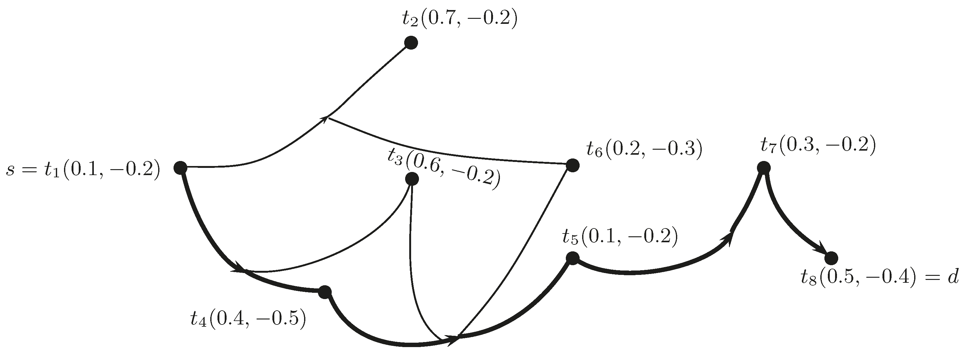
A BF directed hypergraph and a hyperpath between two nodes s and d is shown in Figure 1 (generated with LaTeXDraw 2.0.8 Mon17 October 2016 12:01:25 PDT).
The path is drawn as a thick line.
Definition 7.
[4] The incidence matrix representation of a directed hypergraph is given as a matrix of order , defined as follows:
Definition 8.
The incidence matrix of a BF directed hypergraph is characterized by an matrix as follows:
Definition 9.
Let be a BF directed hypergraph. The height of G is defined as:
where and , is taken as the positive membership value and indicates the negative membership value of vertex i to hyperedge j.
Definition 10.
A BF directed hypergraph is simple if there are no repeated BF hyperedges in U, and if and , then , for each k and j.
Definition 11.
A BF directed hypergraph is called support simple if whenever , and , then , for all i and j. Then, the hyperedges and are called supporting edges.
Definition 12.
A BF directed hypergraph is named elementary if and are constant functions. If , then it is characterized as a spike; that is, a BF subset with singleton support.
Theorem 1.
The BF directed hyperedges of a BF directed hypergraph are elementary.
Example 2.
Consider a BF directed hypergraph , such that , . The corresponding incidence matrix is given in Table 2.
The corresponding elementary BF directed hypergraph is shown in Figure 2.
Definition 13.
Let be a BF directed hypergraph. Suppose that and . The -level is defined as . The crisp directed hypergraph , such that:
- ,
- ,
Definition 14.
Let be a BF directed hypergraph and be the -level directed hypergraphs of G. The sequence of real numbers, where and , , such that the following properties:
- (i)
- if , then ,
- (ii)
- ,
Definition 15.
Let be a BF directed hypergraph and . If for each and each , , for all , then G is sectionally elementary.
Definition 16.
Let be a BF directed hypergraph and . G is said to be ordered if is ordered. That is, . The BF directed hypergraph is called simply ordered if the sequence is simply ordered.
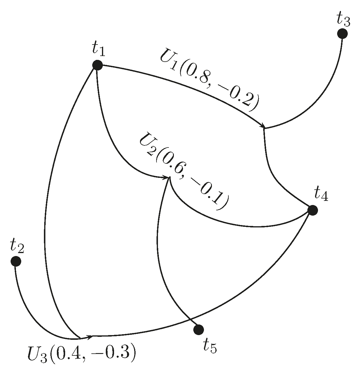
Example 3.
Consider a BF directed hypergraph , such that , , given by the incidence matrix in Table 3.
The corresponding graph is shown in Figure 3.
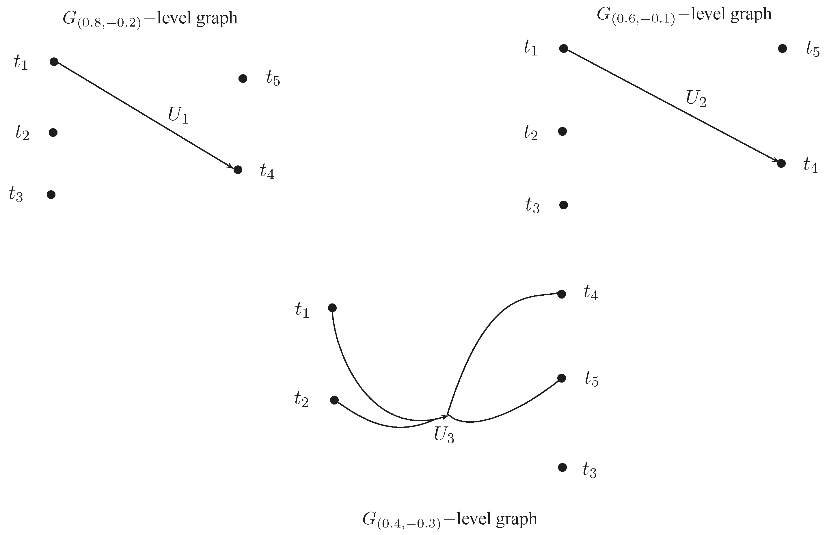
By computing the -level BF directed hypergraphs of G, we have and . Note that and . The fundamental sequence is . The -level is not in . Furthermore, . G is not sectionally elementary since for , . The BF directed hypergraph is ordered, and the set of core hypergraphs is . The induced fundamental sequence of G is given in Figure 4.
Theorem 2.
- (a)
- If is an elementary BF directed hypergraph, then G is ordered.
- (b)
- If G is an ordered BF directed hypergraph with and if is simple, then G is elementary.
We now define the index matrix representation and certain operations on BF directed hypergraphs.
Definition 17.
Let be a BF directed hypergraph. Then, the index matrix of G is of the form as given in Table 4, where and
where and , . The edge between two vertices and is indexed by , whose values can be find out by using the Cartesian products defined below.
Definition 18.
Let E be a fixed set of points. The Cartesian product of two BF sets and over E is defined as:
- .
- .
We now define some operations on BF directed hypergraphs.
Definition 19.
The addition of BF directed hypergraphs and , which is denoted by , is defined as , where:
and:
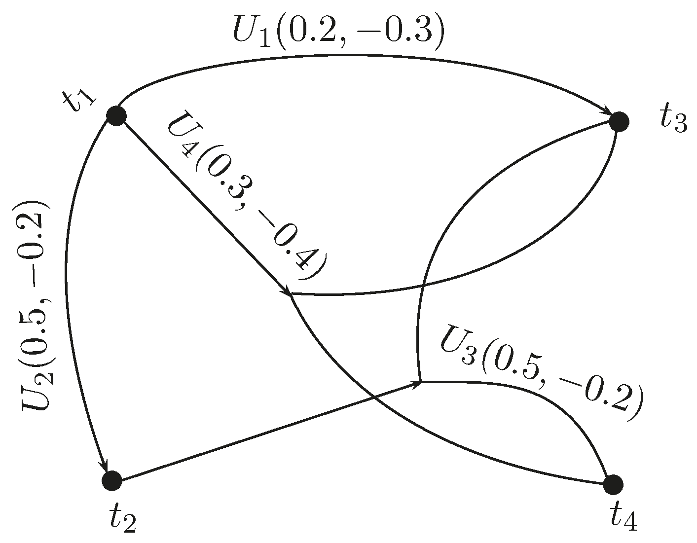
Example 4.
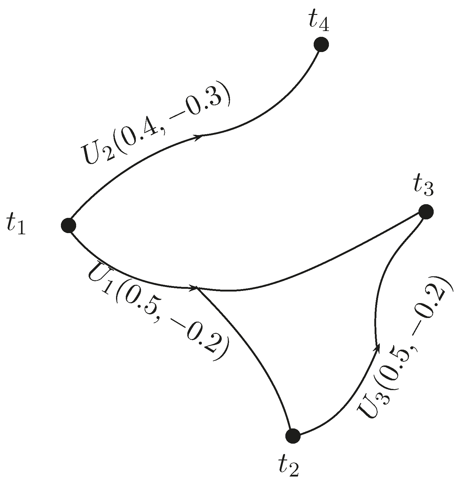
Consider the BF directed hypergraphs and , where , and , as shown in Figure 5 and Figure 6, respectively.
The index matrix of is as given in Table 5, where and:
The index matrix of is as given in Table 6, where and:
The index matrix of is , where . The membership values are calculated by using Equation (1), and are calculated by using Equation (2) and are given in Table 7.
The graph of is shown in Figure 7.
Definition 20.
The vertex-wise multiplication of two BF directed hypergraphs and , denoted by , is , where:
Example 5.
Consider BF directed hypergraphs and as shown in Figure 5 and Figure 6, respectively. The index matrix of is , where . The membership values are calculated by using Equation (3), and are calculated by using Equation (4) and are given in Table 8.
The graph of is given in Figure 8.
Definition 21.
The multiplication of two BF directed hypergraphs and , denoted by , is defined as , where:
and:
Remark 1.
The positive membership and negative membership values of the loops in the resultant graph (if present) can be calculated as or and or .
Example 6.
The index matrix of graph is , where . The membership values are calculated by using Equation (5), and are calculated by using Equation (6) and are given in Table 9.
The graph of is shown in Figure 9.
Definition 22.
The structural subtraction of and , denoted by , is defined as , where “−” is the set theoretic difference operation and:
If , then the graph of is also empty.
Example 7.
Consider BF directed hypergraphs and as shown in Figure 5 and Figure 6. The index matrix of is , where . The membership values are calculated by using Equation (7), and are calculated by using Equation (8) and are given in Table 10.
The following Figure 10 shows their structural subtraction.
Definition 23.
A BF directed hypergraph is called -tempered BF directed hypergraph of if there exists a crisp hypergraph and a BF set , such that , where:
Let denotes the B-tempered hypergraph of G, which is firmed by the crisp hypergraph and the BF set .
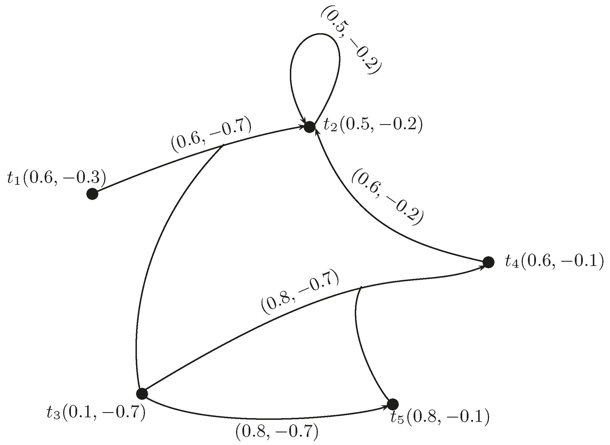
Example 8.
Consider the BF directed hypergraph , where and ; the corresponding incidence matrix is given in Table 11.
The corresponding graph is shown in Figure 11.
Then, , .
Define by , , , , , , , .
Note that:
Thus:
Hence, G is a B-tempered BF directed hypergraph.
Theorem 3.
A BF directed hypergraph is a -tempered BF directed hypergraph determined by some crisp hypergraph if and only if G is elementary, simply ordered and support simple.
Proof.
Suppose that is a B-tempered BF directed hypergraph, which is firmed by some crisp hypergraph . Since G is B-tempered, then the positive membership values and negative membership values of BF directed hyperedges are the same. Hence, G is elementary. If the support of two BF directed hyperedges of the B-tempered BF directed hypergraph is the same, then the BF hyperedges are equal. Hence, G is support simple. Let . Since G is elementary, it will be ordered.
Claim: G is simply ordered.
Let , then there exists , such that and . Since and , it follows that and . Hence, G is simply ordered.
Conversely, suppose is elementary, simply ordered and support simple. As we know, and and are defined by:
To prove , where:
Let .
There is a unique BF hyperedge in U having support because G is elementary and support simple. Clearly, different edges in U having distinct supports lie in . We have to prove that for each , , . Since distinct edges have different supports and all edges are elementary, then the definition of the fundamental sequence implies that is the same as an arbitrary element of of . Therefore, . Further, if , then . Since , the definition of B-tempered indicates that for each , and .
To prove and for some , it follows from the definition of B-tempered and for all and, so, . Since G is simply ordered, therefore , which is a contradiction to the definition of B-tempered BF directed hypergraphs. Thus, from the definition of and , we have , . ☐
Theorem 4.
Let be a simply-ordered BF directed hypergraph and . If is a simple hypergraph, then there exists a partial BF directed hypergraph of G, such that the conditions given below are satisfied:
- (i)
- is a B-tempered BF directed hypergraph of G.
- (ii)
- , that is for all , there exist , such that and .
- (iii)
- and .
Proof.
By the above Theorem, we have G is an elementary BF directed hypergraph. By the removal of all of those edges of G which lie in another edge of G properly, we attain the partial BF directed hypergraph , where and , then . Since is simple and all of its edges are elementary, no edges can properly be contained in other edges of G if they have different support. Hence, (iii) holds. We know that is support simple. Thus, all of the above conditions are satisfied by . From the definition of , is elementary and support simple. Thus, is B-tempered. ☐
3. Algorithm For Computing Minimum Arc Length and Shortest Hyperpath
This section investigates the definition of the triangular BF number. The score and ranking of BF numbers are also defined. A triangular BF number is used to represent the arc length in a hypernetwork. The algorithm explained below is based on [16]. Let denotes the arc length of the j -th hyperpath.
Definition 24.
Let E be a finite set, which is non-empty, and be a BF set. Then, the pair is called a BF number, denoted by , where , , .
Definition 25.
A triangular BF number B is denoted by , where and are BF numbers. Therefore, a triangular BF number is given by . The diagrammatic representation of BF number is shown in Figure 12.
Definition 26.
Let be a triangular BF number, then the score of is a BF set whose positive membership value is and negative membership value is .
Definition 27.
The accuracy of a triangular BF number is defined as .
| Algorithm 1. |
| Input. Enter the number of hyperpaths and their membership values, which are taken as triangular BF number. |
| Output. Minimum arc length of BF directed hypernetwork. |
| 1. Calculate the lengths of all possible hyperpaths for where |
| 2. Initialize . |
| 3. Set . |
| 4. The positive membership values are computed as |
| , |
| , |
| and negative membership values as |
| . |
| 5. Set , as calculated in Step 4. |
| 6. |
| 7. If , then stop the procedure. If , then go to Step 3. |
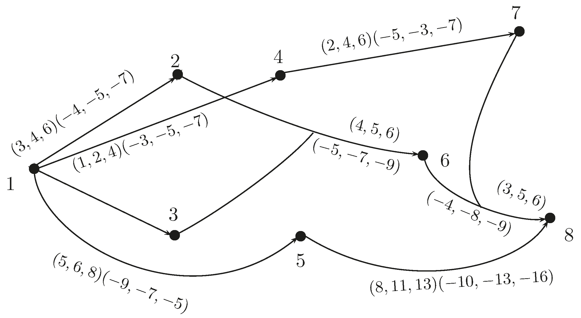
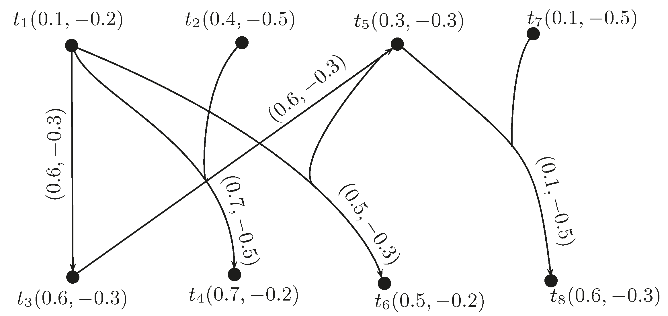
Example 9.
Consider a hypernetwork with triangular BF arc lengths shown in Figure 13.
(1) From source Vertex 1 to destination Vertex 8, there are four possible paths , given as follows:
- Path(1): , ;
- Path(2): , ;
- Path(3): , ;
- Path(4): , .
(2) Initialize .
(3) Initialize .
(4) Let and . Compute the positive membership values as:
and negative membership values as:
(5) Set .
(6) .
(7) If , go to Step 4.
(4) Let and . Calculate the positive membership values as:
and negative membership values as:
(5) Set .
Repeat the procedure until .
Finally, we get the minimum arc length of BF hypernetwork as:
We now write steps of the score-based method to determine a BF shortest hyperpath.
- (1)
- All possible hyperpaths are considered from the source point to the destination.
- (2)
- Compute the scores of the hyperpaths.
- (3)
- Find the accuracy of all paths.
- (4)
- The shortest hyperpath is obtained with the lowest accuracy.
Example 10.
Consider the BF hypernetwork as +shown in Figure 13. The BF shortest hyperpath in this hypernetwork is recognized using the score-based method. The scores of hyperpaths can be calculated a 6s:
Similarly, and .
The accuracy of hyperpaths can be computed as:
From Table 12 given below, the path with minimum accuracy is identified as the BF shortest hyperpath.
4. Conclusions
BF graph theory is widely applied in computer science and mathematics. In comparison to the classical and fuzzy models, BF models provide more precision, comparability and flexibility to the system as they combine the bipolarity and fuzziness both into a unified model. We have represented the BF directed hypergraphs using the incidence matrix and described their certain properties. We have represented the BF directed hypergraphs using the index matrix. We have described certain operations on BF directed hypergraphs, including addition, multiplication and structural subtraction. We have discussed an algorithm to find the minimum arc length of the BF directed hyperpath. We aim to widen our research work to: (1) BF soft directed hypergraphs; (2) bipolar neutrosophic hypergraphs; (3) rough neutrosophic graphs; and (4) soft rough directed hypergraphs.
Author Contributions
Both authors contributed equally to this manuscript.
Conflicts of Interest
The authors declare that there are no conflicts of interest regarding this manuscript.
References
- Berge, C. Graphs and Hypergraphs; North-Holland Publishing Company: Amsterdam, The Netherlands, 1973. [Google Scholar]
- Liu, D.R.; Wu, M.Y. A hypergraph based approach to declustering problems. Distrib. Parallel Databases 2001, 10, 269–288. [Google Scholar] [CrossRef]
- Ausiello, G.; Nanni, U.; Italiano, G.F. Dynamic maintenance of directed hypergraphs. Theor. Comput. Sci. 1990, 72, 97–117. [Google Scholar]
- Gallo, G.; Longo, G.; Pallottin, S. Directed hypergraphs and applications. Discret. Appl. Math. 1993, 42, 177–201. [Google Scholar]
- Zadeh, L.A. Fuzzy sets. Inf. Control 1965, 8, 338–353. [Google Scholar]
- Zhang, W.-R. Bipolar fuzzy sets and relations: A computational framework forcognitive modeling and multiagent decision analysis. In Proceedings of the Fuzzy Information Processing Society Biannual Conference, San Antonio, TX, USA, 18–21 December 1994; pp. 305–309.
- Kaufmann, A. Introduction a la Theorie des Sous-Ensembles Flous; Masson et Cie: Paris, France, 1973. [Google Scholar]
- Zadeh, L.A. Similarity relations and fuzzy orderings. Inf. Sci. 1971, 3, 177–200. [Google Scholar]
- Rosenfeld, A. Fuzzy graphs. In Fuzzy Sets and Their Applications; Zadeh, L.A., Fu, K.S., Shimura, M., Eds.; Academic Press: New York, NY, USA, 1975; pp. 77–95. [Google Scholar]
- Bhattacharya, P. Some remarks on fuzzy graphs. Pattern Recogn. Lett. 1987, 6, 297–302. [Google Scholar]
- Mordeson, J.N.; Chang-Shyh, P. Operations on fuzzy graphs. Inf. Sci. 1994, 79, 159–170. [Google Scholar]
- Mordeson, J.N.; Nair, P.S. Fuzzy Graphs and Fuzzy Hypergraphs, 2nd ed.; Physica Verlag: Heidelberg, Germany, 2001. [Google Scholar]
- Chen, S.M. Interval-valued fuzzy hypergraph and fuzzy partition. IEEE Trans. Syst. Man Cybern. Part B 1997, 27, 725–733. [Google Scholar]
- Lee-Kwang, H.; Lee, K.-M. Fuzzy hypergraph and fuzzy partition. IEEE Trans. Syst. Man Cybern. 1995, 25, 196–201. [Google Scholar]
- Parvathi, R.; Thilagavathi, S. Intuitionistic fuzzy directed hypergraphs. Adv. Fuzzy Sets Syst. 2013, 14, 39–52. [Google Scholar]
- Rangasamy, P.; Akram, M.; Thilagavathi, S. Intuitionistic fuzzy shortest hyperpath in a network. Inf. Process. Lett. 2013, 113, 599–603. [Google Scholar]
- Myithili, K.K.; Parvathi, R.; Akram, M. Certain types of intuitionistic fuzzy directed hypergraphs. Int. J. Mach. Learn. Cybern. 2016, 7, 287–295. [Google Scholar]
- Akram, M. Bipolar fuzzy graphs. Inf. Sci. 2011, 181, 5548–5564. [Google Scholar]
- Akram, M.; Dudek, W.A. Regular bipolar fuzzy graphs. Neural Comput. Appl. 2012, 21, 197–205. [Google Scholar]
- Akram, M.; Waseem, N. Novel applications of bipolar fuzzy graphs to decision making problems. J. Appl. Math. Comput. 2016. [Google Scholar] [CrossRef]
- Sarwar, M.; Akram, M. Novel concepts of bipolar fuzzy competition graphs. J. Appl. Math. Comput. 2016. [Google Scholar] [CrossRef]
- Samanta, S.; Pal, M. Bipolar fuzzy hypergraphs. Int. J. Fuzzy Log. Syst. 2012, 2, 17–28. [Google Scholar]
- Akram, M.; Dudek, W.A.; Sarwar, S. Properties of bipolar fuzzy hypergraphs. Ital. J. Pure Appl. Math. 2013, 31, 141–160. [Google Scholar]
- Han, Y.; Shi, P.; Chen, S. Bipolar-valued rough fuzzy set and its applications to decision information system. IEEE Trans. Fuzzy Syst. 2015, 23, 2358–2370. [Google Scholar]
- Shi, P.; Su, X.; Li, F. Dissipativity-based filtering for fuzzy switched systems with stochastic perturbation. IEEE Trans. Autom. Control 2016, 61, 1694–1699. [Google Scholar]
- Shi, P.; Zhang, Y.; Chadli, M.; Agarwal, R. Mixed H-infinity and passive filtering for discrete fuzzy neural networks with stochastic jumps and time delays. IEEE Trans. Neural Netw. Learn. Syst. 2016, 27, 903–909. [Google Scholar]
Figure 1.
A path from source s to destination node d in a BF set directed hypergraph.

Figure 2.
Elementary BF directed hypergraph.

Figure 3.
BF directed hypergraph.

Figure 4.
G induced fundamental sequence.

Figure 5.
.

Figure 6.
.

Figure 7.
.
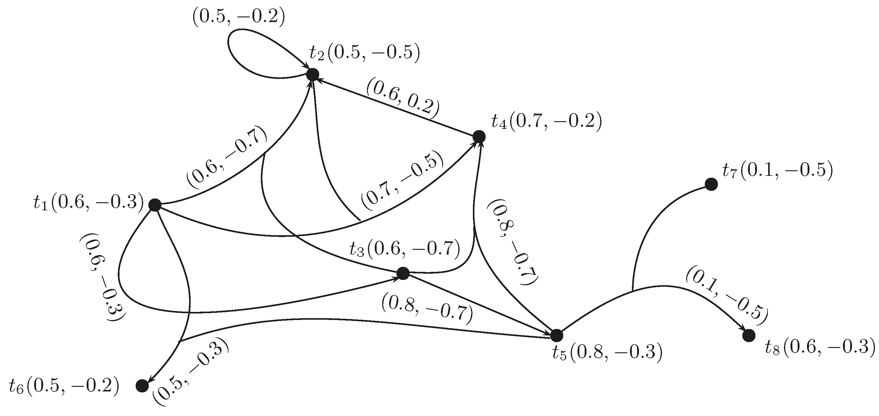
Figure 8.
.
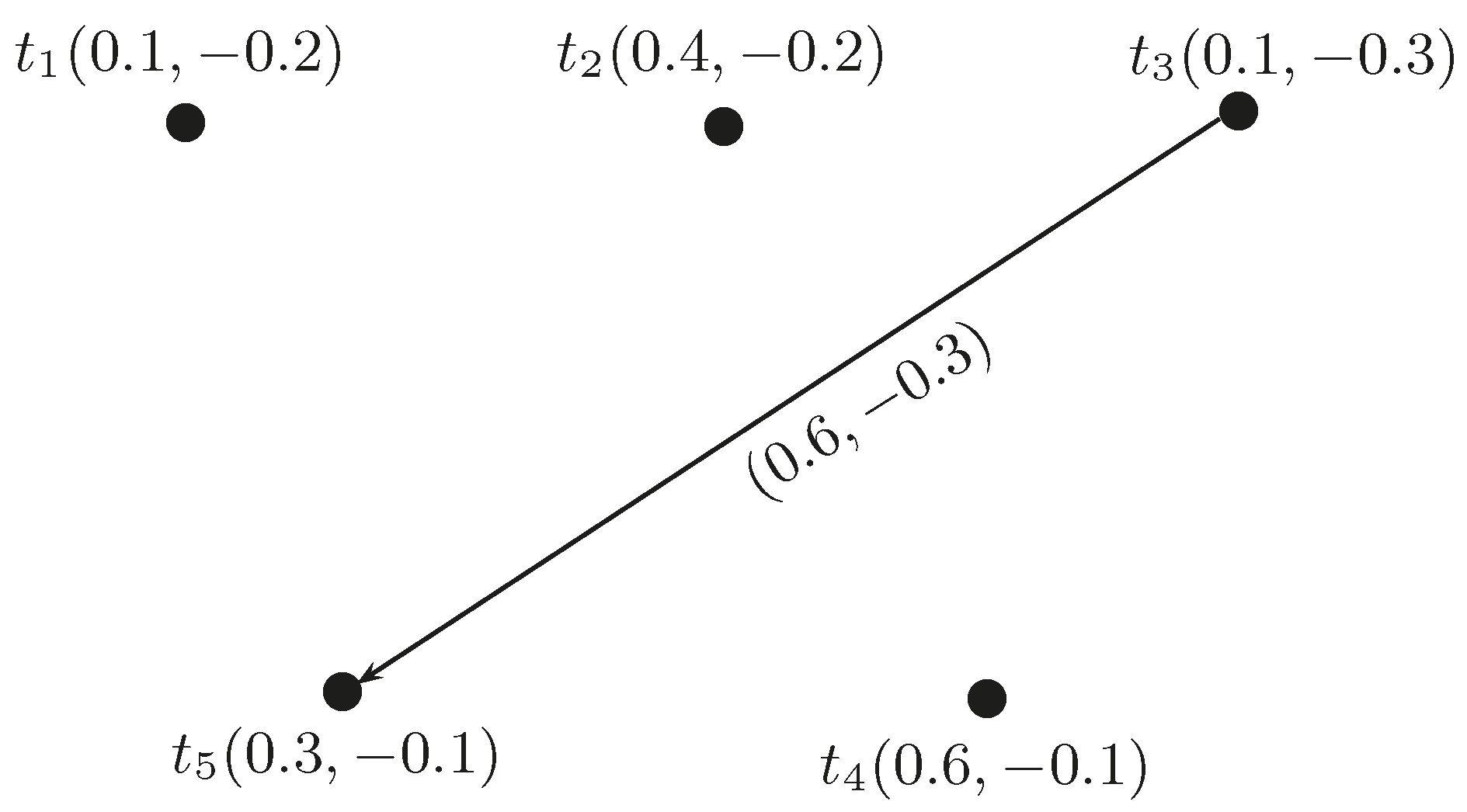
Figure 9.
.
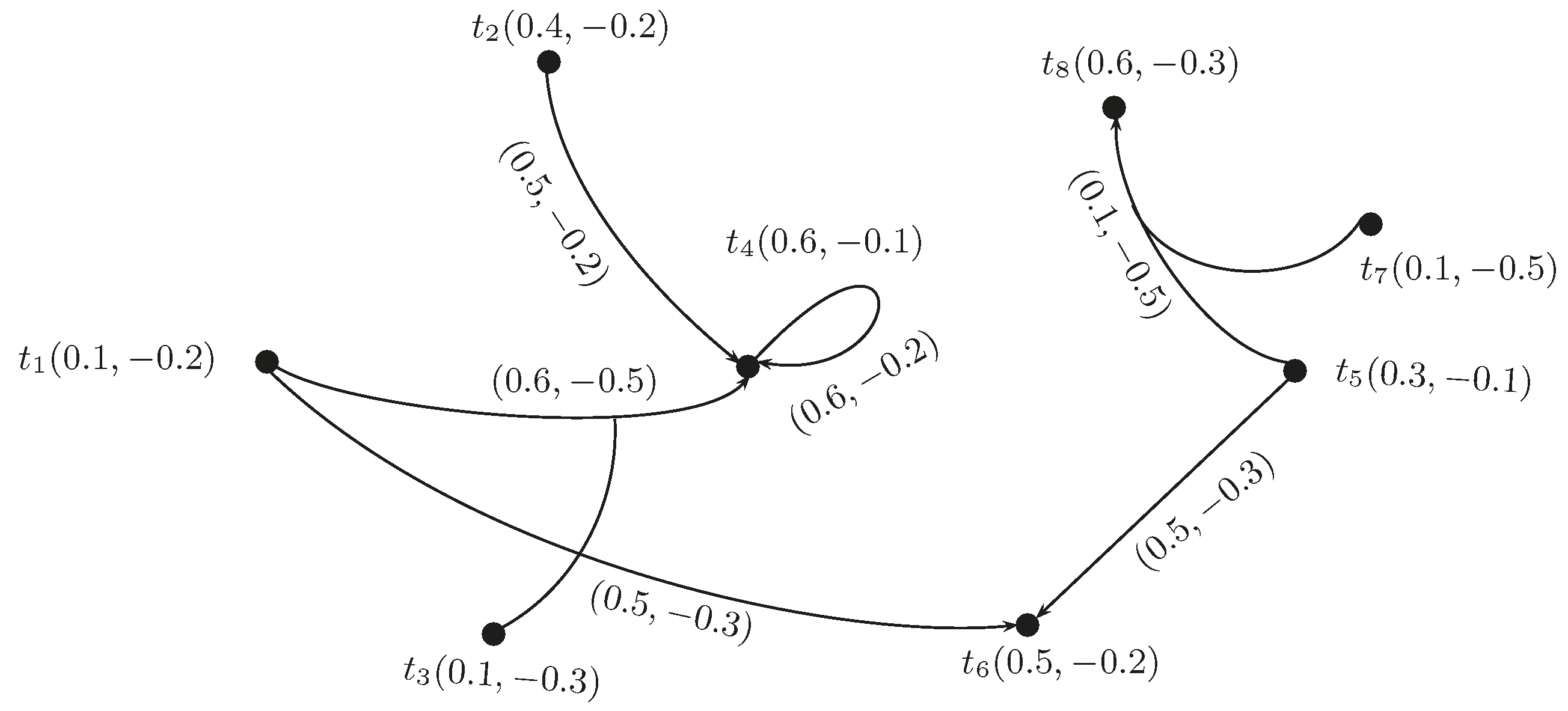
Figure 10.
.
Figure 11.
B-tempered BF directed hypergraph.

Figure 12.
Triangular BF number.
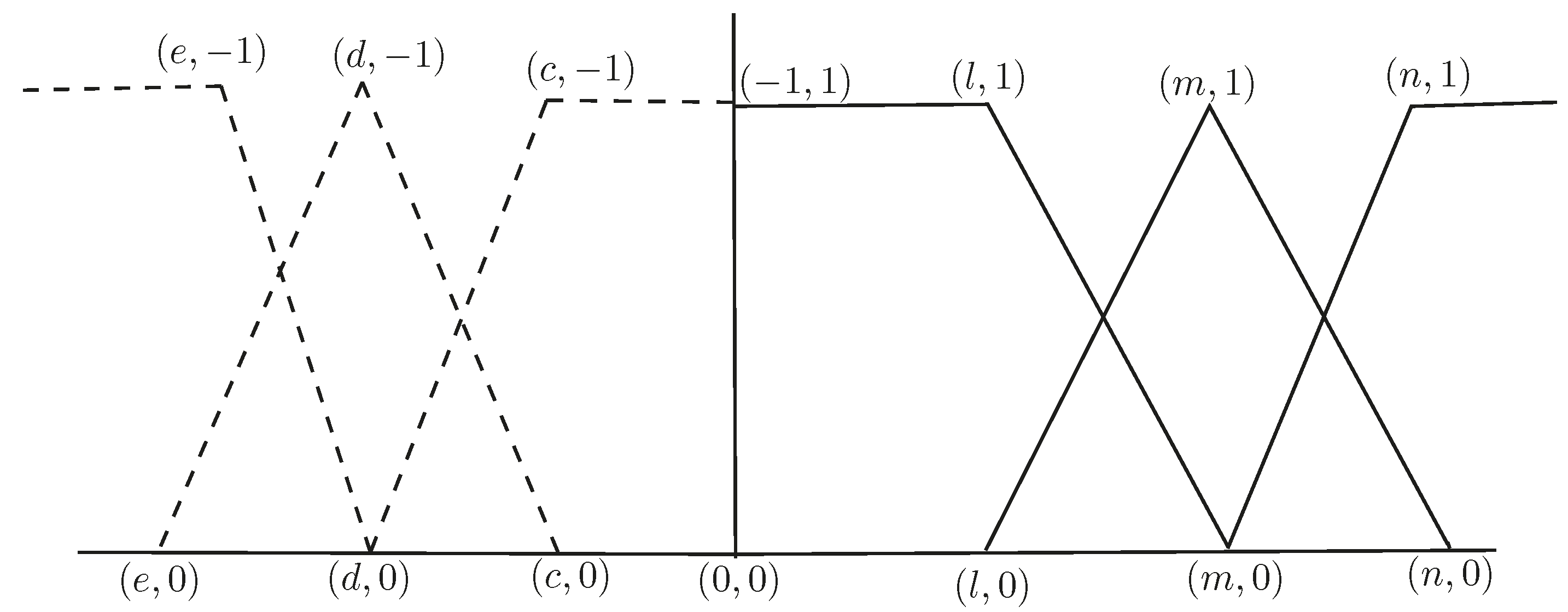
Figure 13.
BF hypernetwork.

| Notations | Description |
|---|---|
| BF set | |
| BF directed hypergraph having vertex set T and edge set U | |
| Index matrix of G | |
| Triangular BF number | |
| Score of BF number | |
| Accuracy of BF number | |
| Height of hypergraph G | |
| Fundamental sequence of G | |
| Core set of G | |
| -level BF hypergraph |
| I | ||||
|---|---|---|---|---|
| I | |||
|---|---|---|---|
| ⋯ | ||||
|---|---|---|---|---|
| ⋯ | ||||
| ⋯ | ||||
| ⋮ | ⋮ | ⋮ | ⋮ | ⋮ |
| ⋯ |
| = | |||||||||
| 0 | 0 | 0 | 0 | 0 | 0 | 0 | 0 | ||
| 0 | 0 | 0 | 0 | 0 | 0 | 0 | 0 | ||
| 0 | 0 | 0 | 0 | 0 | 0 | 0 | |||
| 0 | 0 | 0 | 0 | 0 | 0 | ||||
| 0 | 0 | 0 | 0 | 0 | 0 | 0 | |||
| 0 | 0 | 0 | 0 | 0 | 0 | ||||
| 0 | 0 | 0 | 0 | 0 | 0 | 0 | 0 | ||
| 0 | 0 | 0 | 0 | 0 | 0 |
| 0 | 0 | 0 | 0 | 0 | ||
| 0 | ||||||
| 0 | 0 | 0 | 0 | 0 | ||
| 0 | 0 | 0 | ||||
| 0 | 0 | 0 | 0 |
| 0 | 0 | 0 | 0 | 0 | 0 | 0 | 0 | ||
| 0 | 0 | 0 | 0 | ||||||
| 0 | 0 | 0 | 0 | 0 | 0 | 0 | |||
| 0 | 0 | 0 | 0 | ||||||
| 0 | 0 | 0 | 0 | 0 | 0 | 0 | |||
| 0 | 0 | 0 | 0 | 0 | 0 | ||||
| 0 | 0 | 0 | 0 | 0 | 0 | 0 | 0 | ||
| 0 | 0 | 0 | 0 | 0 | 0 |
| 0 | 0 | 0 | 0 | 0 | ||
| 0 | 0 | 0 | 0 | 0 | ||
| 0 | 0 | 0 | 0 | 0 | ||
| 0 | 0 | 0 | 0 | 0 | ||
| 0 | 0 | 0 | 0 |
| = | |||||||||
| 0 | 0 | 0 | 0 | 0 | 0 | 0 | 0 | ||
| 0 | 0 | 0 | 0 | 0 | 0 | 0 | 0 | ||
| 0 | 0 | 0 | 0 | 0 | 0 | 0 | 0 | ||
| 0 | 0 | 0 | 0 | ||||||
| 0 | 0 | 0 | 0 | 0 | 0 | 0 | 0 | ||
| 0 | 0 | 0 | 0 | 0 | 0 | ||||
| 0 | 0 | 0 | 0 | 0 | 0 | 0 | 0 | ||
| 0 | 0 | 0 | 0 | 0 | 0 |
| = | ||||
| 0 | 0 | 0 | ||
| 0 | 0 | 0 | ||
| 0 | 0 |
| Path | Score | Accuracy | Rank |
|---|---|---|---|
| 2 | |||
| 3 | |||
| 4 | |||
| 1 |
© 2017 by the authors. Licensee MDPI, Basel, Switzerland. This article is an open access article distributed under the terms and conditions of the Creative Commons Attribution (CC BY) license ( http://creativecommons.org/licenses/by/4.0/).
Share and Cite
MDPI and ACS Style
Akram, M.; Luqman, A. Certain Concepts of Bipolar Fuzzy Directed Hypergraphs. Mathematics 2017, 5, 17. https://doi.org/10.3390/math5010017
AMA Style
Akram M, Luqman A. Certain Concepts of Bipolar Fuzzy Directed Hypergraphs. Mathematics. 2017; 5(1):17. https://doi.org/10.3390/math5010017
Chicago/Turabian StyleAkram, Muhammad, and Anam Luqman. 2017. "Certain Concepts of Bipolar Fuzzy Directed Hypergraphs" Mathematics 5, no. 1: 17. https://doi.org/10.3390/math5010017
Note that from the first issue of 2016, this journal uses article numbers instead of page numbers. See further details here.