
Data Clustering with Quantum Mechanics

1
College of Physics and Optoelectronics, Taiyuan University of Technology, Taiyuan 030024, China
2
Near India Pvt Ltd., No. 71/72, Jyoti Nivas College Road, Koramangala, Bengalore 560095, India
3
EngKraft LLC, 312 Adeline Avenue, San Jose, CA 95136, USA
4
Sherman Visual Lab, Sunnyvale, CA 94085, USA
*
Author to whom correspondence should be addressed.
†
These authors contributed equally to this work.
Mathematics 2017, 5(1), 5; https://doi.org/10.3390/math5010005
Submission received: 8 November 2016
/
Revised: 15 December 2016
/
Accepted: 28 December 2016
/
Published: 6 January 2017
(This article belongs to the Special Issue Numerical Linear Algebra with Applications)
Abstract
:Data clustering is a vital tool for data analysis. This work shows that some existing useful methods in data clustering are actually based on quantum mechanics and can be assembled into a powerful and accurate data clustering method where the efficiency of computational quantum chemistry eigenvalue methods is therefore applicable. These methods can be applied to scientific data, engineering data and even text.
1. Introduction
For any data of a physical or chemical nature, whether they be pharmaceutical data, particle physics, renewable energies, security, the Internet or wireless communications, there is a growing need for data analysis and predictive analytics. Researchers regularly encounter limitations due to large datasets in complex physics simulations, biological and environmental research. One of the biggest problems of data analysis is data with no known a priori structure. Therefore, data clustering, which seeks to find internal classes or structures within the data, is one of the most difficult, yet needed implementations. The standard algorithm is K-means [1], which rests on the following assumptions:
- (1)
- Assume in advance the number of clusters;
- (2)
- Generate random seeds;
- (3)
- Assume at least one seed “hits” every cluster;
- (4)
- Clusters “grow” in the neighborhood of each seed;
- (5)
- Cluster regions grow until saturation.
The algorithm is not stable if the clusters are not clearly distinct; the randomness aspect can create multiple solutions. This is especially true for text when a cluster of words often has a minimal semantic relation with another cluster. For such cases, one has to resort to “fuzzy” clustering. Moreover, if more data are added to the dataset, clustering requires a complete repetition of the K-means approach for the whole dataset. Granted, the literature has many extensions to K-means for determining cluster centers (e.g., [2,3]) and fuzzy clustering (e.g., [4]), but these involve extensions in different directions and always extra computations. Furthermore, additions to the data almost always requires applying the K-means algorithm (standard or extended) all over again. Rather, we desire a simpler, stable, non-random, geometrically-based method that addresses the issues of cluster centers, fuzzy clustering and readily amenable to the addition of data and parallel processing.
On a different note, although the origin of information theory is attributed to Claude Shannon in 1948, the concept of entropy already existed in physics as early as the 19th century in thermodynamics and can be rigorously derived from its mathematical-physical basis, i.e., statistical mechanics. The question of a link between information entropy and thermodynamic entropy is a hotly debated topic [5,6,7,8]. The link between thermodynamics and information entropy was developed in a series of papers by Edwin Jaynes beginning in 1957 [8]. The problem with linking thermodynamic entropy to information entropy is that in information entropy, the entire body of thermodynamics, which deals with the physical nature of entropy, is missing. For example, can such concepts as energy be applied to non-physical datasets formulated by text documents or engineering data?
After a preliminary discussion in Section 2.1 by which we define essential metrics, we present the foundations of our methods for (i) dimensional reduction based on the Meila–Shi algorithm in Section 2.1.2 and (ii) clustering based on the Schrödinger equation in Section 2.1.3. In particular, we show a previously unknown connection between the Meila–Shi algorithm and the conventional Singular Value Decomposition (SVD) used in Principal Component Analysis (PCA). Section 2.2 presents the realization of these methods via computational quantum mechanics, in particular efficient iterative eigenvalue schemes amenable to data updates and the possibilities of parallelization. We illustrate the range of applications by a series of demo examples, as shown in Section 3, including a performance table for dimensional reduction of large datasets. The discussion is provided at the end.
2. Methods
2.1. Theoretical Background
2.1.1. Preliminaries: Definitions of Metrics
The notions of partition functions and free energies have been defined previously, in particular by the work of Buhmann and Hofmann [9,10], used in simulated annealing and elsewhere (e.g., the work of Shenghuo Zhu et al. [11] and also the work of Lafon ([12] (2.10)). In [9,10], Buhmann and Hofmann consider an “energy” defined by the cost function ([9] (4)) for Euclidean pairwise (central) clustering:
where are the d-dimensional vectors representing each data point, define a dissimilarity measure and is a Boolean assignment matrix for the number of K clusters with the restriction and uniqueness for every data point i. From this, in perfect analogy with the definitions in statistical mechanics/thermodynamics, they define a partition function ([9] (6)) by:
and a “free energy” by . The average are given by derivatives of the free energy ([9] (8)) (associated with each set of indices (the beauty of the partition function is that it can often be factored into sub-system components or conversely integrated within larger systems)):
which can be interpreted in the context of fuzzy logic (values between 0 and 1). Buhmann and Hofmann then proceed in considering a partition function for a “free particle contribution” and treat the cost function of the “interaction”, presumably the interaction related to the cost function in Equation (1), by a perturbative scheme carried to first order ([9] Section 3). They consequently optimize the estimated average “energy”. Subsequently, they formulate an optimization problem of a pairwise clustering in the maximum entropy framework using a variational principle to derive data partitionings in a d-dimensional space. Equation (3) will be seen again further on.
2.1.2. Spectral Clustering: Meila–Shi Algorithm
For any real data matrix , the spectral clustering method known as the Meila–Shi algorithm [13] uses:
where is the similarity matrix, is the adjacency matrix and is a row-stochastic matrix, often called a Markov matrix [14]. It is also called a transition matrix and plays an important role in quantum mechanical Monte Carlo calculations [15,16] and fundamental quantum mechanics (see, e.g., [17,18]). Here, and are respectively the normalized eigenvectors of and (taken as column vectors), but these matrices share the same eigenvalues , which have special properties:
However, the corresponding eigenvectors of , i.e., provide a much better clustering picture. For , is a constant vector and represents the data background, which is usually not interesting and can be discarded. This background can correspond to an underlying basis, e.g., in the case of text, the background can result from the repeated use of stop words, like “and” or ”the”, which though frequently used in the English language, do not convey essential information. For , plotting the lead eigenvectors versus (often the leading two eigenvectors are sufficient), serves as the principal axes, graphically provides a clustering picture and, consequently, a considerable dimensional and size reduction of the original problem. The theory behind the Meila–Shi algorithm is justified by graph theory [13] in that it isolates the strongest relationships within a given graph.
Lafon and co-workers have recast the Meila–Shi algorithm through their so-called diffusion maps [12,19] via the Fokker–Planck equation [20], which is formally related to the Schrödinger equation [21,22]. Diffusion maps exploit the relationship between heat diffusion and the random walk Markov chain. This connection is embedded in the diffusion Monte-Carlo method, which is formally the Schrödinger equation in imaginary time and notably one of the most accurate calculation schemes in quantum mechanics [23,24]. In this regard, the leading eigenvalues of in the diffusion scheme are interpreted as representing the “thermodynamic equilibrium of a dynamical system”, while the lesser eigenvalues correspond to the decay modes of a system that is not in equilibrium. This provides a physical picture in helping to understand why only the lead eigenvectors, , where, e.g., only are sufficient for an accurate clustering picture, depending on how rapidly the eigenvalues decrease with increasing index i. From the following definitions [25]:
- Let and be vectors defined by and where is given by Equation (4):
- and are diagonal matrices.
- The matrices and are related to each other by a similarity transformation according to:
Note that in Equation (8) is also equal to:
where c is a constant and . We create a re-normalized like so:
Thus, , and its eigenvectors can be obtained from an SVD [26] like so:
The vectors in are indeed the eigenvectors of from which the eigenvectors of , i.e., can be obtained from the transformation: to within a normalization constant since and share the same eigenvalues and are related to each other by a similarity transformation, e.g., . The matrices and can be reconstructed from the eigenvalues according to:
It is the eigenvectors and from the latter the eigenvectors of , i.e., , that we want. Since we can relate the Meila–Shi algorithm to an SVD, we can identify as principle components of the data representation. However, Section 2.2 shows that the Meila–Shi algorithm is computationally more efficient than an SVD.
2.1.3. Quantum Clustering
Horn and Gottlieb [27,28] took a Parzen window defined by where is a collection of geometrically-defined data points and injected it into the Schrödinger equation:
where is the “kinetic energy operator” or “free particle contribution” as expressed by the Laplacian and where the usual mass term m has been set to unity and the Planck constant term ℏ is replaced by a variance σ. Solving Equation (14) for the potential yields:
Note that the input data points can be, e.g., the outcome of the previous Meila–Shi algorithm. For a regime defined by the variance σ, the cluster centers are the minima of (where a high density of data points is often found). Equation (15) includes the average Boolean assignment terms of Equation (3) from Buhmann and Hofmann [9,10], where Ψ is also identified as a partition function. In principle, the choice of variance can be seen as a bandwidth selection problem in kernel density estimation and can be estimated using a variety of techniques (see, e.g., [29]). Note that Lafon also uses Gaussian functions of the form to determine the connectivity between two data points, i.e., the probability of walking from and in one step of a random walk of his diffusion maps [19].
The right-hand side of Equation (15) provides a clustering mechanism that is more accurate than the standard clustering algorithms like the standard K-means, as we shall see. It is also more stable because it is geometrically invariant in that it does not depend on the order in which data are injected, unlike other clustering methods. It is thus amenable to incremental and distributed systems.
2.2. Computational Aspects
2.2.1. Dimensional Reduction
The decomposition of Equation (12) is computationally expensive. However, the Meila–Shi algorithm relinquishes , which is only needed to construct the matrix, and is consequentially much more computationally efficient. It provides a considerable dimensional reduction of the original data matrix into manageable eigenvectors and, for larger datasets, provides a better clustering picture. It is therefore far more computationally efficient and accurate than the conventional SVD. Moreover, the eigenvalue solvers from state-of-the-art quantum chemistry codes provide very efficient eigenvalue solvers for large sparse matrices.
The advantage of the Meila–Shi algorithm over a conventional SVD is shown by the following complexity analysis (obtained from the tools of Golub and Van Loan [26]):
- SVD:
- For a matrix, the complexity of a full SVD is (this is quoted more often in its “optimized” version as , e.g., see [30], which has a lower complexity for thinner SVDs), and K is expected to be very large for text data, easily the size of a thesaurus of a hundred thousand words. The complexity is roughly cubic in behavior when (note that we rarely need, e.g., in Equation (12) for clustering only the vectors and the eigenvalues , unless we desire to reconstitute ; in this respect, the SVD is overkill).
- Meila–Shi:
- For various cases, the complexity for getting the eigenvalues of the matrix is:where c is the product cost (cost of a scalar multiplication plus a scalar addition).
The complexity is at its lowest for large sparse matrices. Quantum chemistry has motivated the development of scalable fast and efficient eigenvalue solvers. Amongst the best eigenpair (eigenvalue with eigenvector) solvers for large sparse matrices is the Jacobi–Davidson algorithm [31,32], which has proven to be fast and robust. Similar to the Lanczos’ method, Davidson’s method is an iterative projection method that however does not take advantage of Krylov subspaces, but uses the Rayleigh–Ritz procedure with non-Krylov spaces and expands the search spaces in a different way. It has been successfully applied to ab initio quantum chemistry calculations [33]. The best and most general eigenpair solver using the Jacobi–Davidson scheme is the PRIMMEcode [34], and it is amenable to parallel processing. PRIMME is a comprehensive combination of various methods, and their interplay and comparison to other methods have already been examined [35].
As the data matrix is upgraded with new documents (new data), this combined iterative scheme should readily adjust to the new matrix with minimal computations. In particular, we do not want to compute and store , nor in virtual memory, since we must avoid the storage of (which might be on a distributed network). For larger datasets, becomes more dense and impossible to contain within the maximum allowable RAM. We present two ways of dealing with this:
- Returning to the standard SVD on as defined in Equation (12), we define a symmetric matrix from the non-symmetric matrix as:The eigenvectors of have the form ([36] (p. 3)):where will contain the leading eigenvectors (equal to ) of the matrix . is then subjected to the eigenpair solver. The above also applies for the eigenpairs of , since we have established the connection between , , and in Equations (11) and (12) in Section 2.1.2 on the Meila–Shi algorithm. The eigenvalues of (which are the same as those for ) are the square root of the eigenvalues of , normalized so that the first (or zeroth eigenvalue) is unity. We call this the “B method”, as tabulated in Table 1.
- Since it is the eigenpairs of Λ that we want, the matrix-vector multiplication routine is done in two steps:where is a temporary vector. This two-step process performs . We call this the “ method” as also tabulated it in Table 1.
In the case of a matrix , where , the second method performs better while requiring less memory. Once the eigenvectors for either a conventional SVD or the Meila–Shi algorithm are obtained, we can obtain clusters via the Quantum Clustering (QC) method.
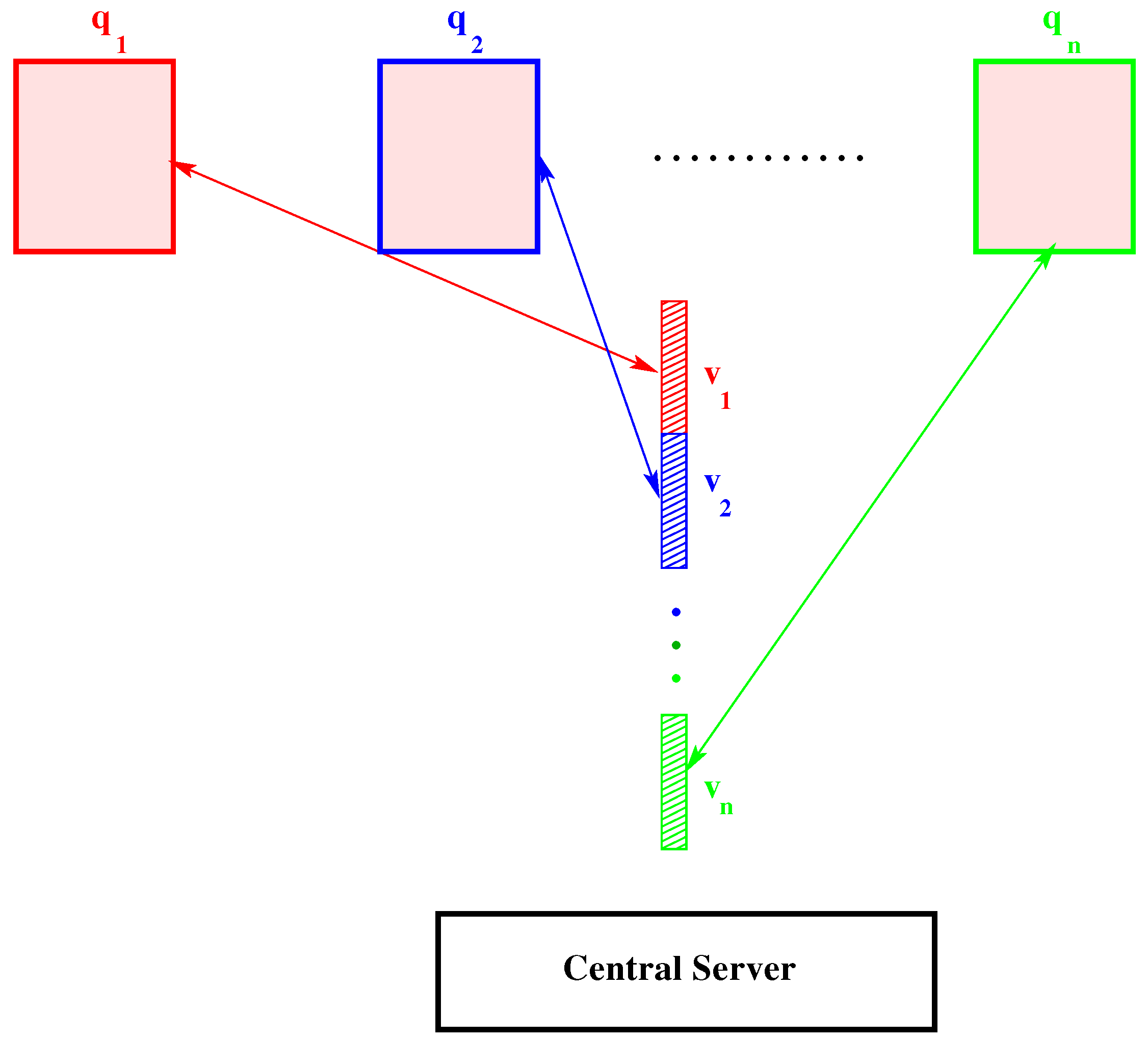
One can do even better with a distributed system with parallel processing (e.g., see [37]). Consider Figure 1, where the data on each server/node denoted for stay put, but a signal is sent from a central server and calculations applied to the data in each node, producing a “signature”. All of the signatures are collected in a central server, which contains the entire eigenvector. This scheme also allows for additional data, i.e., rank-one updates, where the previous set of eigenvectors serve as guesses for the next iteration. The messages passing between nodes can be done by MPI (Message Passing Interface) with the signatures collected from each node possibly through Map-Reduce [38].
2.2.2. Finding the Minima of Quantum Potential
The sums needed for computing the QC potential of Equation (15) are readily amenable to vectorization and parallel computation, as well as the addition of data. An iterative Newton–Raphson scheme for finding the minima of the QC potential, which correspond to the cluster centers, is needed to determine the cluster centers and, thus, clustering itself. Although the gradient descent method has been used by Horn et al. [28] to find local minima of the quantum potential, the Broyden–Fletcher–Goldfarb–Shanno (BFGS) algorithm is more efficient and scales well. The data points themselves can serve as initial guesses in this scheme (as evidenced by many test runs with COMPACT [28]). In practice, this scheme works well and does not need graphical visualization, but some improvements are needed: this Newton–Raphson scheme does mathematically guarantee all of the potential minima. The only known case of systems by which all of the cluster centers can be obtained involve polynomial systems. However, the quantum potential includes Gaussian functions. If two eigenvectors from the Meila–Shi algorithm are sufficient, a two-dimensional visualization is possible, but graphical analysis of every single dataset by a person does not translate into automatic program control.
3. Results
3.1. Examples
3.1.1. K-Means vs. Quantum Clustering
This first example is composed of artificially-created random points within two circular envelopes of different sizes with the circle of a smaller size having a high density of points. Figure 2a shows the result for K-means, as provided by the MATLAB toolbox, for a choice of two clusters. The result here is stable, but illustrates one of the problems experienced with overlapping clusters using K-means. The smaller cluster, shown in red, penetrates the larger circle too much. However, as shown in Figure 2b, the contour plot of the quantum potential allows us to better isolate the smaller cluster (where the cluster centers are shown in black dots). The continuous transitions between potential minima, which are the cluster centers, provide a continuous description of the “fuzzy-clustering” aspects.
3.1.2. Rock Crabs
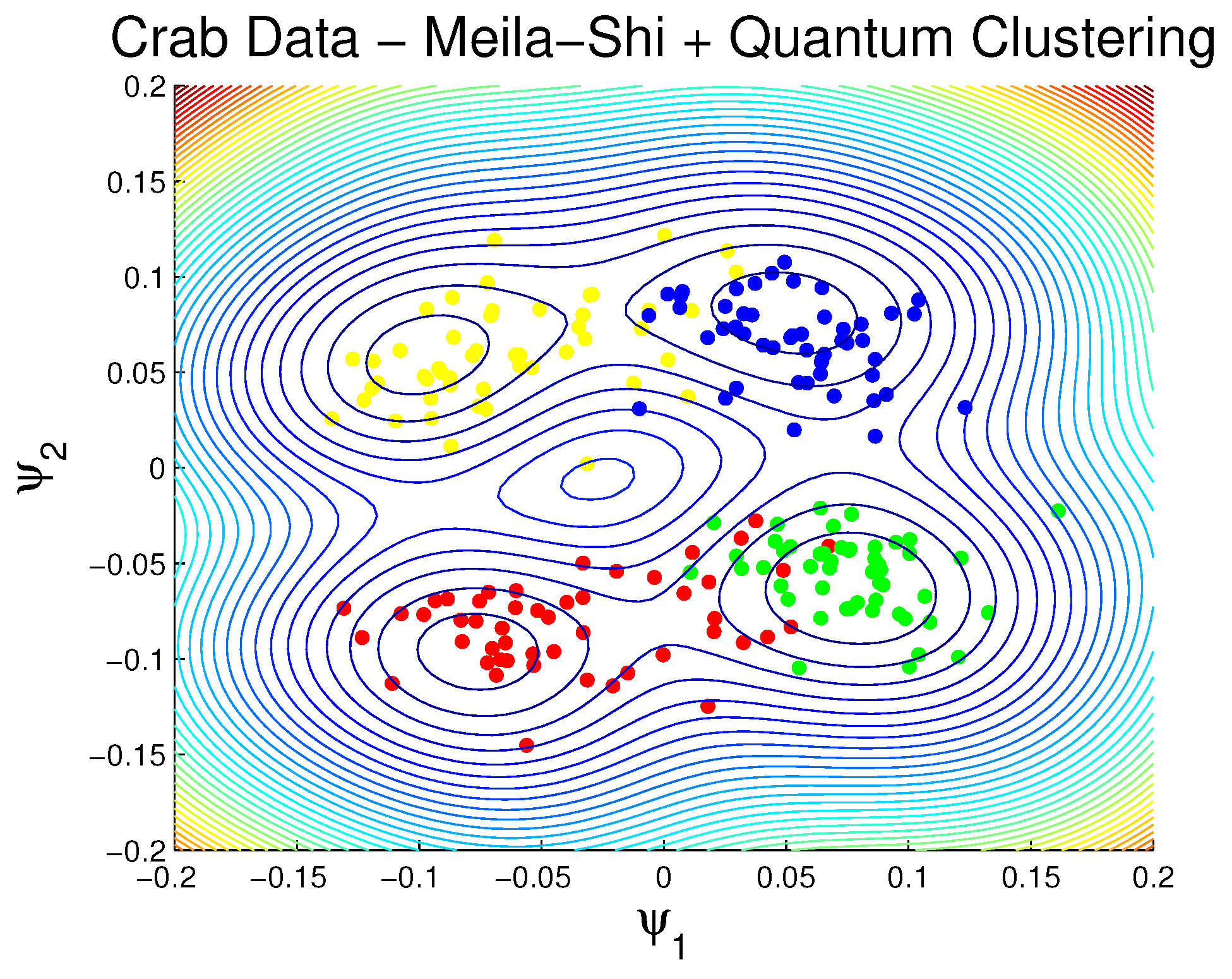
This second example from biology was the first application of the quantum clustering method [27,39,40]. One had two sexes and two (new) species and consequently four groups. Preserved specimens lost their color, so it was hoped that morphological differences would enable museum material to be classified. Data were collected on 50 specimens of each sex of each species, collected in Western Australia. Each specimen had measurements according to: (1) frontal lip (2) rear width (3) length along midline (4) maximum width of carapace and (5) body depth. Thus, the total dataset is a data matrix. Figure 3 shows the outcome of the application of spectral (Meila–Shi) and quantum clusterings on this data. The actual classes are illustrated by the colors red, blue, green and yellow. The lead eigenvectors and are sufficient to provide a complete two-dimensional clustering picture. Also shown is the contour plot from the quantum clustering potential, the minima clearly indicating the cluster centers. All four classes were recovered to within of the data according to the Jaccard index [41].
The “fuzzy” nature of points that are nearly equally spaced between cluster centers is handled continuously by the quantum potential of Equation (15). Whereas Horn and Gottlieb use the SVD to obtain their principle components (e.g., see the applications of their software called COMPACT [28]), we used instead the Meila–Shi algorithm. Our results are comparable, but the difference in outcome between the two approaches increases for larger datasets (in both row and column size).
3.1.3. Finding Clues of a Disease
It becomes important to establish that our clustering methods can be applied to man-made problems and especially, as we will see later here, text. This is an example of “detective” work with clues written as text. Purely empirical experimentation is slow and costly. Preliminary and on-going analyses can optimize efforts. One attempts to form hypotheses about disease, or pain, or discomfort in order to track down their source and potential. In this example, we look for the causes of migraine headaches through the analysis of medical evidence. These clues are written according to the following list of one-line documents [42]:
- (1)
- stress is associated with migraines;
- (2)
- stress can lead to loss of magnesium;
- (3)
- calcium channel blockers prevent some migraines;
- (4)
- magnesium is a natural calcium channel blocker;
- (5)
- Spreading Cortical Depression (SCD) is implicated in some migraines;
- (6)
- high levels of magnesium inhibit SCD;
- (7)
- migraine patients have high platelet aggregability;
- (8)
- magnesium can suppress platelet aggregability.
These text documents are converted into numbers using a “bag-of-words” model shown previously, i.e., the data matrix is defined according to:
where is the number of times the j-th term appearing in the i-th document. We cluster according to the terms, and thus, instead of Equation (4); but like the previous example, we get Figure 4. Here, σ is chosen so that only one cluster is produced. As we can see from the contour plot, the terms “magnesium” (in red) and “migraine” (in yellow) are very near to the cluster center at the center of the MATLAB contour plot, suggesting that magnesium deficiency may play a role in migraine headaches. Note that the colored lines represent the gradation of the MATLAB contour plot. This hypothesis was confirmed by experiment. We can also discern three clusters in Figure 4 and realize their themes with the following. The concept of an object (a document or a document set) can be thought of as its Boolean representation in the “term space” [43]. It shows if the object contains the given term (yes or no). It does not care about the actual frequency of the term in the object. For example: for
It resembles the occupation number representation of fermions in the Fock space of quantum field theory. The scheme of “thematic clustering” [44] is to represent the theme of a cluster, by re-arranging term-labels by their total frequency in the cluster, and then print out, say, the top 10 words after mapping the term-label back to the term (word). This allows one to cluster this dataset into the following:
- (1)
- Documents 5 and 6: high levels of magnesium inhibit spreading cortical depression (SCD), which is implicated in some migraines.
- (2)
- Documents 3 and 4: magnesium is a natural calcium channel blocker that prevents some migraines.
- (3)
- Documents 1, 2, 7 and 8:
- (a)
- tress is associated with migraines and can lead to loss of magnesium.
- (b)
- migraine patients have high platelet aggregability, which can be suppressed by magnesium.
Thematic clustering combines information retrieval with quantum field theory to find themes or concepts to clusters and thereby refine them.
3.1.4. Artificial X–Y Pairs with Gaussian Variance
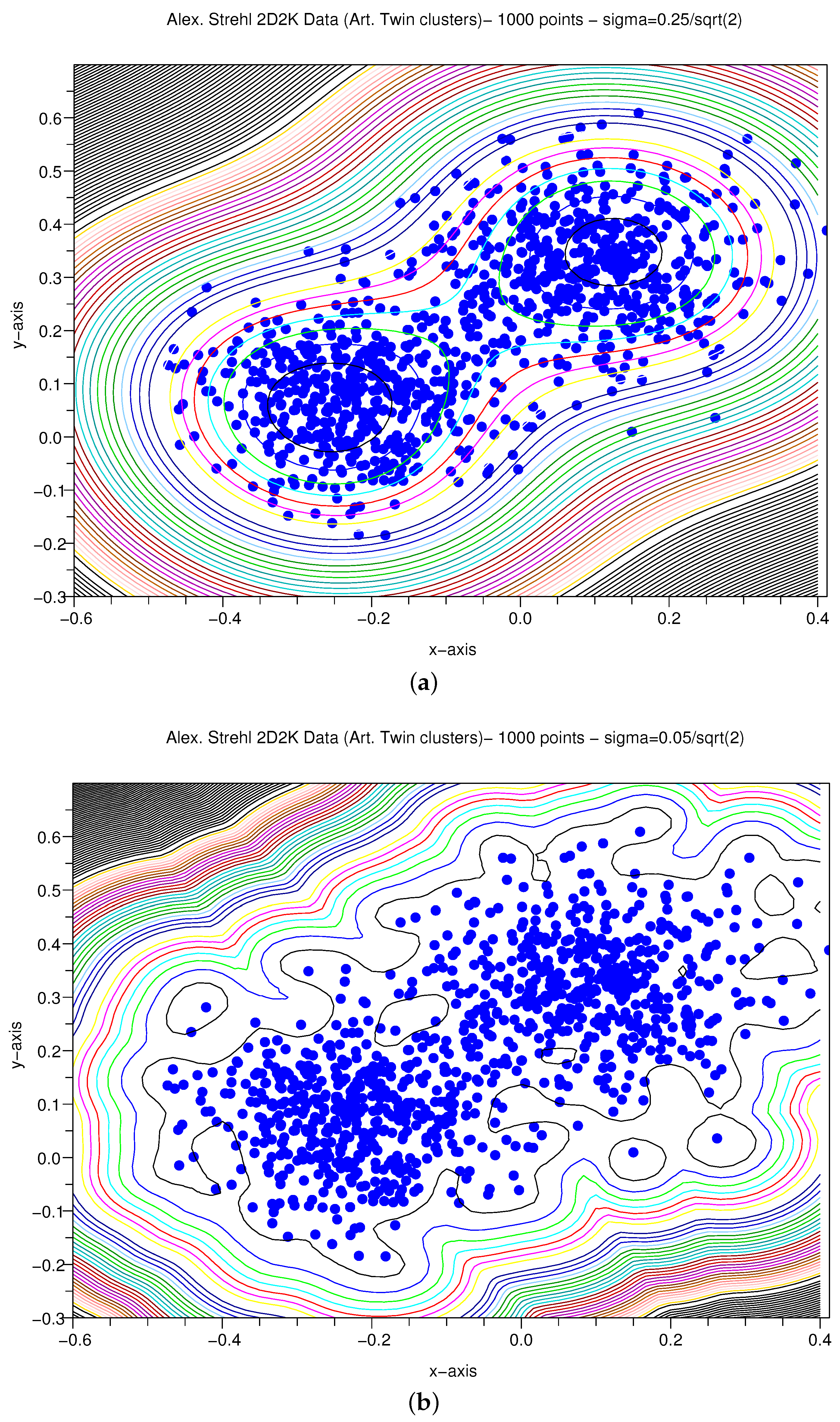
The following data are taken from the web-site of Alexander Strehl [45], i.e., a data matrix containing two Gaussians (500 points each). Note that the clusters are not linearly separable in two dimensions. These are Gaussian clusters with a variance of and with means and . This dataset illustrates that not only can our clustering methods handle more than a few hundred points with good continuity, but also how the variation of the scaling factor σ affects the clustering. We considered two values of σ:
The first case shown in Figure 5a shows two clusters. An even smaller value of σ as shown in Figure 5b shows smaller structures, and we can see tight clustering around the points. Thus, the QC method is very much a natural clusterer. It is a matter of selecting the scaling parameter σ for the right regime.
The quantum clustering can be viewed as the inverse operation of the machine learning method-based Support Vector machines (SVM) when using Gaussian kernel functions. This can be understood in the context of Support Vector Clustering (SVC) [46], which appeared before the QC method, the latter being proposed as both an extension of the ideas of SVC and also an alternative [47]. Whereas the SVM using Gaussians to establish regions on space surrounding selected and distinct regions, the quantum clustering instead finds the regions within data for which there is little or no a priori information.
3.1.5. Engineering Data Demo
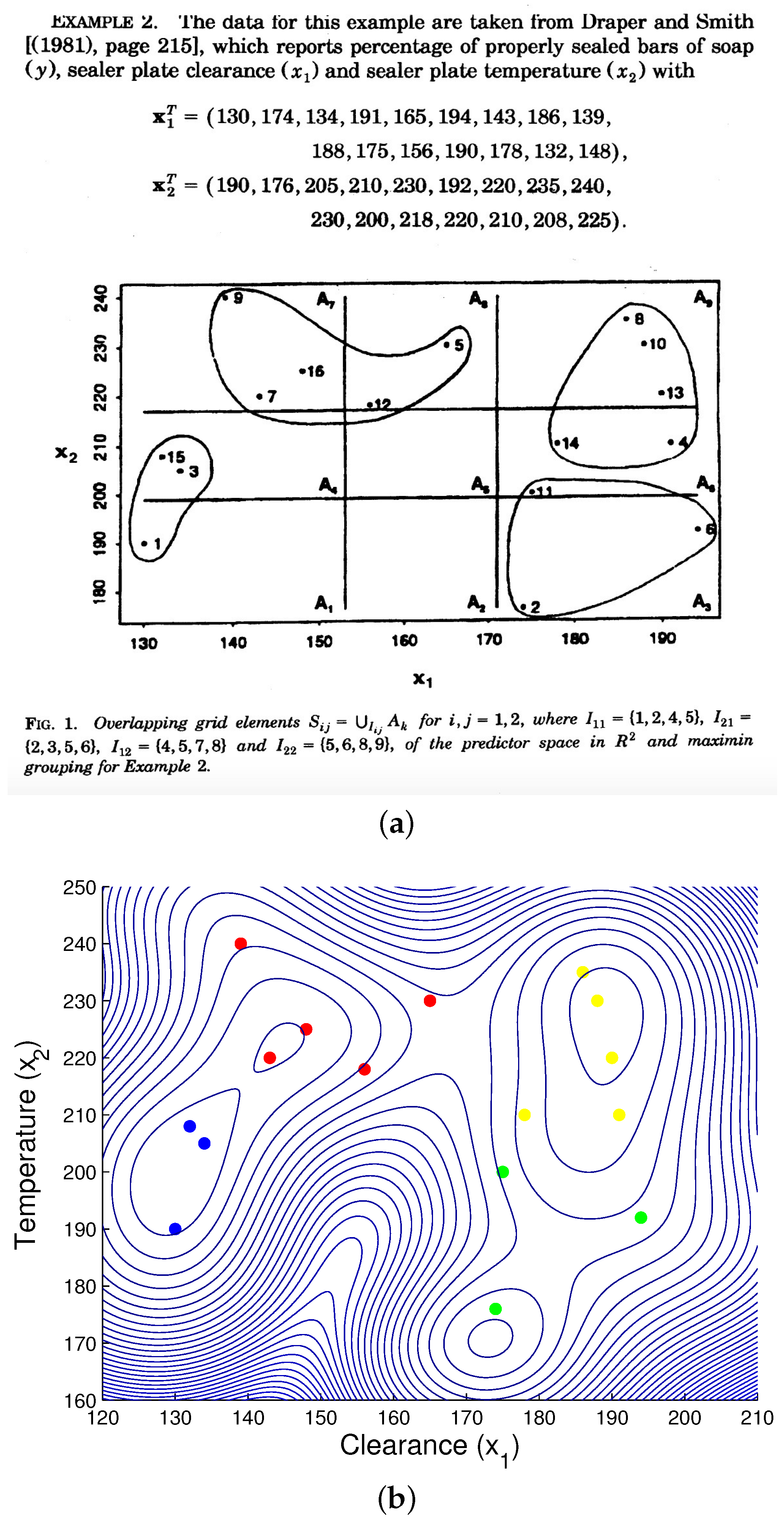
The data for this example are taken from Draper and Smith [48]. They report percentages of properly sealed bars of soap, sealer plate clearance and sealer plate temperature . The latter two variables were measured with 16 pairs. One can view engineering data as a “semi-natural problem” (man-made engineering applied to a natural or scientific problem). We reproduce page 1425 of [49] as shown in Figure 6b.
This shows the clusters successfully obtained by the maximin method. The maximin clustering is widely used and has been applied with success to a variety of problems, such as artificial problems, like imaging systems. The maximin method uses non-linear (constrained) optimization often requiring computational tools, such as linear programming. Though our QC method is conceptually simpler, it nonetheless yields the same clusters as shown in Figure 6b. The reader should not be mistaken by the apparent discrepancy for Points 6 and 11. The contour plot of the potential V should not be confused with the clustering method: it merely illustrates the cluster centers. Points 6 and 11 are closer to the cluster centroid in the bottom right of the picture than the upper right of the picture.
3.1.6. Exoplanet Data
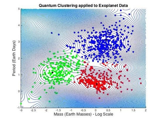
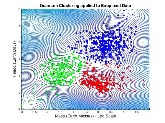
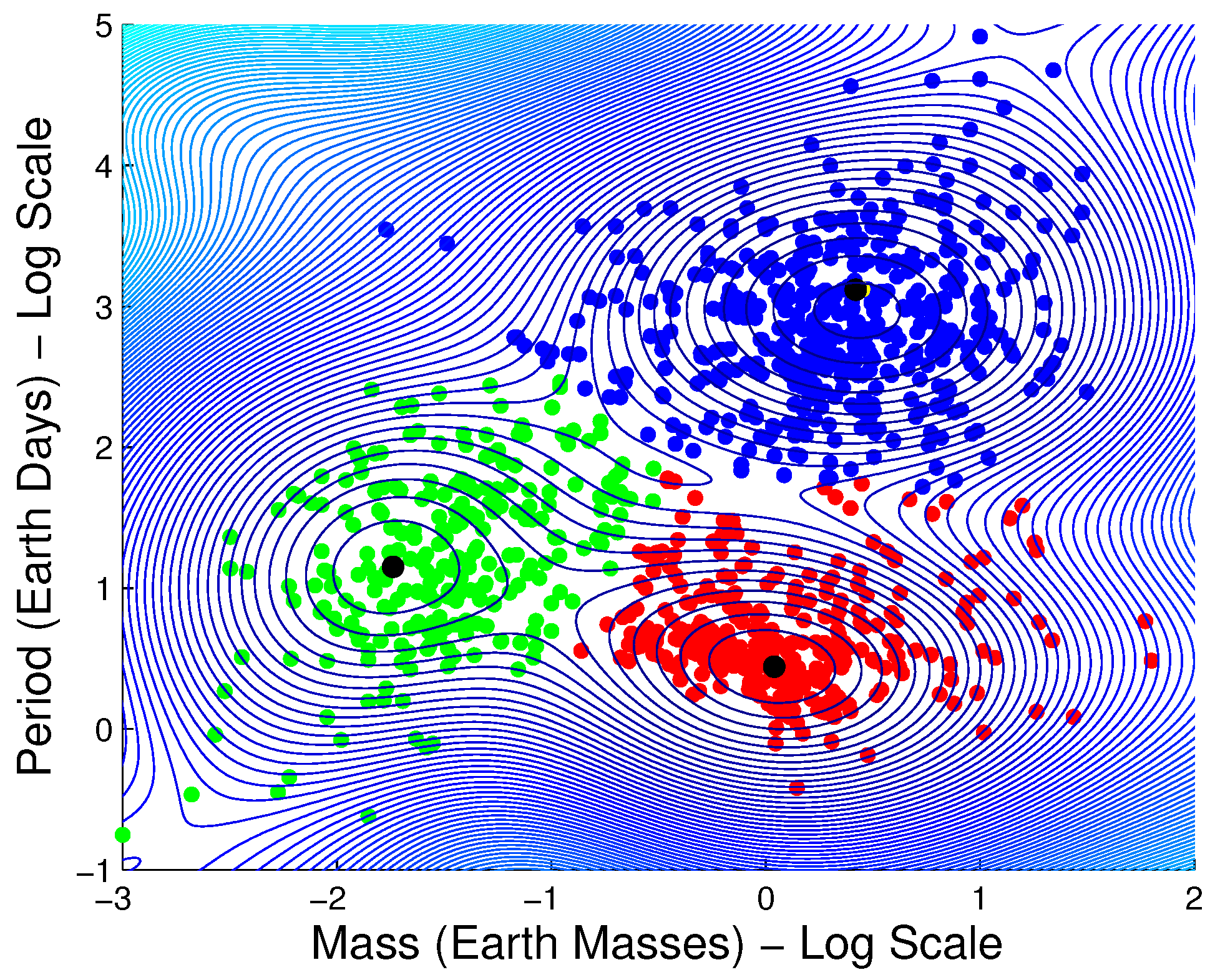
A major astronomical breakthrough of our time is the ongoing discovery of new planets outside our solar system, called exoplanets. Exoplanets are not at all like the nine local planets of our solar system that we know, so well. A first step in the process of understanding the exoplanets might be to try to classify them with respect to their known properties. Data are from the “Extrasolar Planets Encyclopedia” [50]. Figure 7 reproduced from Tahir Yaqoob’s reference [51] is a plot of mass in Earth units versus the period in Astronomical Units (AU) on a log base 10 scale. It shows some very complex behavior, but three rather well-defined groups of data can be discerned. The data cluster on the lower right-hand side corresponds to the massive, short-period hot Jupiters that have been discovered. The points in black are centers computed from the minima of the quantum potential of the QC method.
3.2. PRIMME Test Cases of the Meila–Shi algorithm
Herein, the Meila–Shi algorithm was shown for the small crab and disease demo problems, and thus, we consider the following benchmark results obtained during our experiments with much larger real-world data related to the Patent [52]:
- Reuters:
- 2742 articles from Reuters, 21,578 test set.
- Enron:
- 55,365 email documents, 121,415 distinct terms, sparse data matrix of eight million non-zero entries (density is ).
- user60784:
- documents from website search on a particular person.
- Bill mark:
- test case for web-search on keywords “bill mark” [53].
The Reuters and Enron data were tokenized (and stemmed) using MATLAB TMG [54]. The results for dimensional reduction to the leading eigenvectors were obtained on an Intel(R) Xeon(R) 64-bit, 2400 MHz, 4096 KB cache and are shown in Table 1. The timings for dimensional reduction result from a C/C++ implementation of the PRIMME code. The timings are very small given that they were obtained on a single processor. For rank-one updates, it was found that when increasing the row dimension of the data matrix from N to , the previous eigenvector of length N needed only to be extended, i.e., perturbed [55], to the length with, e.g., starting random numbers, and PRIMME would converge to the new eigenvector within only a few iterations.
With the enclosed demo examples, we have shown that our method of dimensional reduction and the geometrically-based Quantum Clustering method (QC) can naturally cluster data originating from a number of sources whether they be: scientific (natural), engineering and even text. It is understood that first, one uses dimensional reduction, i.e., the Meila–Shi algorithm, before injecting the lead eigenvectors of the resulting transition matrix into the QC method (Some caveats are in order. Though high-powered quantum chemistry techniques can readily obtain the lead eigenvectors for datasets corresponding to large sparse matrices, it is not likely that a blind input of all at once into the QC technique will be useful for, e.g., text with . In this case, one usually obtains concentrated points in the form of “onion peels” of varying density. The QC technique needs to be applied selectively or recursively to these “onion peels” and yield a hierarchy of clusters, as our methods are amenable to iteration.). The choice of the variance σ for the QC clustering is first obtained by obtaining the range of the boundaries surrounding the data. In practice, a circular range of radius R yields an initial guess for . The latter can be reduced, e.g., successfully divided according to until clusters are found.
We find that the interdisciplinary methods in data analysis like the Meila–Shi algorithm, Support Vector Clustering (SVC) and certainly the quantum clustering method of Horn and co-workers, when using Gaussian functions as the common mathematical denominator, are quantum mechanical from a computational point of view. Thus, we can exploit computationally-efficient quantum chemistry methods, such as the most efficient eigenvalue solvers and matrix algebra, which allow us to enlarge the domain the investigations allowed in conventional applications of quantum mechanics. Furthermore, solutions in terms of Gaussian functions involve the most developed mathematical “technology” of quantum chemistry (e.g., the Gaussian program [56]). This “technology” can be exploited in the data clustering methods shown herein.
In the case of text, the hard part is no longer the clustering once geometrically meaningful data points are obtained: it is the encoding leading to that geometrically-meaningful data. Nonetheless, the “bag-of-words” model as shown for the disease potential case was shown to be effective.
We have also outlined an algorithm for distributed data networks, which involves the addition of documents. It is based on iterative or incremental clustering where the eigenvectors are updated via efficient successive updates, including rank-one updates for additional data. At no point is the large matrix (dataset) entirely contained within, e.g., virtual memory. Rather, one needs instead to calculate the outcome of a matrix-vector operation involving a large matrix with elements generated on-the-fly and whose outcome is a (manageable) vector.
The applications envisaged in science alone, especially for data from experiment or measurement, are nearly endless: climate/weather, nuclear decay, mathematical chemistry, genetic studies and more. With the availability of new disparate data sources from multiple domains, a reliable and scalable clustering technique is essential by which to discover and hypothesize new relations during the course of exploratory data analysis.
Acknowledgments
Tony C. Scott was supported in China by the project GDW201400042 for the “high end foreign experts project”. We thank Haricharan Aragonda of Near.co and Greg Fee of CECMat Simon Fraser university for helpful feedback. We would also like to thank YuncaiWang of Taiyuan University of Technology (TYUT) for supporting this work. Wang is supported by the National Natural Science Foundation of China under Grant No. 61405138, No. 61475111 and No. 61227016, by the Program for the Outstanding Innovative Teams of Higher Learning Institutions of Shanxi.
Author Contributions
Tony C. Scott assembled the building blocks of the theory and devised the MATLAB code for the tests based on biological, engineering and physical examples. Madhu Therani provided text-based examples and the means, material resources and support for all calculations. Xiang Wang invented the thematic clustering applied to text-based examples.
Conflicts of Interest
The authors declare no conflict of interest.
References
- Lloyd, S.P. Least squares quantization in PCM. IEEE Trans. Inform. Theory 1982, 28, 129–137. [Google Scholar] [CrossRef]
- Huang, M.; Yu, L.; Chen, Y. Improved K-Means Clustering Center Selecting Algorithm. In Information Engineering and Applications, Proceedings of the International Conference on Information Engineering and Applications (IEA 2011), Chongqing, China, 21–24 October 2011; Zhu, R., Ma, Y., Eds.; Springer: London, UK, 2012; pp. 373–379. [Google Scholar]
- Girisan, E.; Thomas, N.A. An Efficient Cluster Centroid Initialization Method for K-Means Clustering. Autom. Auton. Syst. 2012, 4, 1. [Google Scholar]
- Dunn, J.C. A Fuzzy Relative of the ISODATA Process and Its Use in Detecting Compact Well-Separated Clusters. J. Cybernet. 1973, 3, 32–57. [Google Scholar] [CrossRef]
- Brillouin, L. Science and Information Theory; Academic Press: Dover, UK, 1956. [Google Scholar]
- Georgescu-Roegencholas, N. The Entropy Law and the Economic Process; Harvard University Press: Cambridge, MA, USA, 1971. [Google Scholar]
- Chen, J. The Physical Foundation of Economics—An Analytical Thermodynamic Theory; World Scientific: London, UK, 2005. [Google Scholar]
- Lin, S.K. Diversity and Entropy. Entropy 1999, 1, 101–104. [Google Scholar] [CrossRef]
- Buhmann, J.M.; Hofmann, T. A Maximum Entropy Approach to Pairwise Data Clustering. In Conference A: Computer Vision & Image Processing, Proceedings of the 12th IAPR International Conference on Pattern Recognition, Jerusalem, Israel, 9–13 October 1994; IEEE Computer Society Press: Hebrew University, Jerusalem, Israel, 1994; Volume II, pp. 207–212. [Google Scholar]
- Hofmann, T.; Buhmann, J.M. Pairwise Data Clustering by Deterministic Annealing. IEEE Trans. Pattern Anal. Mach. Intell. 1997, 19, 1–14. [Google Scholar] [CrossRef]
- Zhu, S.; Ji, X.; Xu, W.; Gong, Y. Multi-labelled Classification Using Maximum Entropy Method. In Proceedings of the 28th Annual International ACM SIGIR Conference on Research and Development in Information (SIGIR’05), Salvador, Brazil, 15–19 August 2005; pp. 207–212.
- Coifman, R.R.; Lafon, S.; Lee, A.B.; Maggioni, M.; Nadler, B.; Warner, F.; Zucker, S. Geometric Diffusions as a Tool for Harmonic Analysis and Structure Definition of Data: Diffusion Maps. Proc. Natl. Acad. Sci. USA 2005, 102, 7426–7431. [Google Scholar] [CrossRef] [PubMed]
- Meila, M.; Shi, J. Learning Segmentation by Random Walks. Neural Inform. Process. Syst. 2001, 13, 873–879. [Google Scholar]
- Markov Chains. Applied Probability and Queues; Springer: New York, NY, USA, 2003; pp. 3–38. [Google Scholar]
- Hammond, B.L.; Lester, W.A.; Reynolds, P.J. EBSCOhost. In Monte Carlo Methods in Ab Initio Quantum Chemistry; World Scientific: Singapore; River Edge, NJ, USA, 1994; pp. 287–304. [Google Scholar]
- Lüchow, A. Quantum Monte Carlo methods. Wiley Interdiscip. Rev. Comput. Mol. Sci. 2011, 1, 388–402. [Google Scholar] [CrossRef]
- Park, J.L. The concept of transition in quantum mechanics. Found. Phys. 1970, 1, 23–33. [Google Scholar] [CrossRef]
- Louck, J.D. Doubly stochastic matrices in quantum mechanics. Found. Phys. 1997, 27, 1085–1104. [Google Scholar] [CrossRef]
- Lafon, S.; Lee, A.B. Diffusion maps and coarse-graining: a unified framework for dimensionality reduction, graph partitioning, and data set parameterization. IEEE Trans. Pattern Anal. Mach. Intell. 2006, 28, 1393–1403. [Google Scholar] [CrossRef] [PubMed]
- Nadler, B.; Lafon, S.; Coifman, R.R.; Kevrekidis, I.G. Diffusion maps, spectral clustering and eigenfunctions of fokker-planck operators. In Advances in Neural Information Processing Systems 18; MIT Press: Cambridge, MA, USA, 2005; pp. 955–962. [Google Scholar]
- Bogolyubov, N., Jr.; Sankovich, D.P. N. N. Bogolyubov and Statistical Mechanics. Russ. Math. Surv. 1994, 49, 19. [Google Scholar]
- Brics, M.; Kaupuzs, J.; Mahnke, R. How to solve Fokker-Planck equation treating mixed eigenvalue spectrum? Condens. Matter Phys. 2013, 16, 13002. [Google Scholar] [CrossRef]
- Lüchow, A.; Scott, T.C. Nodal structure of Schrüdinger wavefunction: General results and specific models. J. Phys. B: At. Mol. Opt. Phys. 2007, 40, 851. [Google Scholar] [CrossRef]
- Lüchow, A.; Petz, R.; Scott, T.C. Direct optimization of nodal hypersurfaces in approximate wave functions. J. Chem. Phys. 2007, 126, 144110. [Google Scholar] [CrossRef] [PubMed]
- Cheng, D.; Vempala, S.; Kannan, R.; Wang, G. A Divide-and-merge Methodology for Clustering. In Proceedings of the Twenty-fourth ACM SIGMOD-SIGACT-SIGART Symposium on Principles of Database Systems (PODS ’05), Baltimore, MD, USA, 13–17 June 2015; ACM: New York, NY, USA, 2005; pp. 196–205. [Google Scholar]
- Golub, G.H.; Van Loan, C.F. Matrix Computations. In Johns Hopkins Studies in the Mathematical Sciences; The Johns Hopkins University Press: Baltimore, MD, USA; London, UK, 1996. [Google Scholar]
- Horn, D.; Gottlieb, A. Algorithm for data clustering in pattern recognition problems based on quantum mechanics. Phys. Rev. Lett. 2002, 88, 18702. [Google Scholar]
- COMPACT Software Package. Available online: http://adios.tau.ac.il/compact/ (accessed on 3 January 2017).
- Jones, M.; Marron, J.; Sheather, S. A brief survey of bandwidth selection for density estimation. J. Am. Stat. Assoc. 1996, 91, 401–407. [Google Scholar] [CrossRef]
- Brand, M. Fast low-rank modifications of the thin singular value decomposition. Linear Algebra Appl. 2006, 415, 20–30. [Google Scholar] [CrossRef]
- Sleipjen, G.L.G.; van der Vorst, H.A. A Jacobi-Davidson iteration method for linear eigenvalue problems. SIAM J. Matrix Anal. Appl. 1996, 17, 401–425. [Google Scholar]
- Steffen, B. Subspace Methods for Large Sparse Interior Eigenvalue Problems. Int. J. Differ. Equ. Appl. 2001, 3, 339–351. [Google Scholar]
- Voss, H. A Jacobi–Davidson Method for Nonlinear Eigenproblems. In Proceedings of the 4th International Conference on Computational Science (ICCS 2004), Kraków, Poland, 6–9 June 2004; Bubak, M., van Albada, G.D., Sloot, P.M.A., Dongarra, J., Eds.; Springer: Berlin/Heidelberg, Germany, 2004; pp. 34–41. [Google Scholar]
- Stathopoulos, A. PReconditioned Iterative MultiMethod Eigensolver. Available online: http://www.cs.wm.edu/~andreas/software/ (accessed on 3 January 2017).
- Stathopoulos, A.; McCombs, J.R. PRIMME: Preconditioned Iterative Multimethod Eigensolver—Methods and Software Description. ACM Trans. Math. Softw. 2010, 37, 1–29. [Google Scholar] [CrossRef]
- Larsen, R.M. Computing the SVD for Large and Sparse Matrices, SCCM & SOI-MDI. 2000. Available online: http://sun.stanford.edu/~rmunk/PROPACK/talk.pdf (accessed on 3 January 2017).
- Chen, W.Y.; Song, Y.; Bai, H.; Lin, C.J.; Chang, E.Y. Parallel Spectral Clustering in Distributed Systems. IEEE Trans. Pattern Anal. Mach. Intell. 2011, 33, 568–586. [Google Scholar] [CrossRef] [PubMed]
- Zhang, B.; Estrada, T.; Cicotti, P.; Taufer, M. On Efficiently Capturing Scientific Properties in Distributed Big Data without Moving the Data: A Case Study in Distributed Structural Biology using MapReduce. In Proceedings of the 16th IEEE International Conferences on Computational Science and Engineering (CSE), Sydney, Australia, 3–5 December 2013; Available online: http://mapreduce.sandia.gov/ (accessed on 3 January 2017).
- Ripley, B. Pattern Recognition and Neural Networks; Cambridge University Press: Cambridge, UK, 1996. [Google Scholar]
- Ripley, B. CRAB DATA, 1996. Available online: http://www.stats.ox.ac.uk/pub/PRNN/ (accessed on 3 January 2017).
- Jaccard, P. Etude comparative de la distribution florale dans une portion des Alpes et des Jura. Bull. Soc. Vaud. Sci. Nat. 1901, 37, 547–579. [Google Scholar]
- Hearst, M. Untangling Text Data Mining, 1999. Available online: http://www.ischool.berkeley.edu/~hearst/papers/acl99/acl99-tdm.html (accessed on 3 January 2017).
- Wang, S. Thematic Clustering and the Dual Representations of Text Objects; Sherman Visual Lab. Available online: http://shermanlab.com/science/CS/IR/ThemCluster.pdf (accessed on 2 January 2017).
- Wang, S.; Dignan, T.G. Thematic Clustering. U.S. Patent 888,665,1 B1, 11 November 2014. [Google Scholar]
- Strehl, A. strehl.com. Available online: http://strehl.com/ (accessed on 3 January 2017).
- Ben-Hur, A.; Horn, D.; Siegelmann, H.T.; Vapnik, V. Support Vector Clustering. J. Mach. Learn. Res. 2002, 2, 125–137. [Google Scholar] [CrossRef]
- Dietterich, T.G.; Ghahramani, Z. (Eds.) The Method of Quantum Clustering. In Advances in Neural Information Processes; MIT Press: Cambridge, MA, USA, 2002.
- Draper, N.; Smith, H. Applied Regression Analysis, 2nd ed.; Wiley: New York, NY, USA, 1981. [Google Scholar]
- Miller, F.R.; Neill, J.W.; Sherfey, B.W. Maximin Clusters from near-replicate Regression of Fit Tests. Ann. Stat. 1998, 26, 1411–1433. [Google Scholar]
- Expoplanet.eu—Extrasolar Planets Encyclopedia. Exoplanet Team, Retrieved 16 November 2015. Available online: http://exoplanet.eu/ (accessed on 2 January 2017).
- Yaqoob, T. Exoplanets and Alien Solar Systems; New Earth Labs (Education and Outreach): Baltimore, MD, USA, 16 November 2011. [Google Scholar]
- Fertik, M.; Scott, T.; Dignan, T. Identifying Information Related to a Particular Entity from Electronic Sources, Using Dimensional Reduction and Quantum Clustering. U.S. Patent 8,744,197, 3 June 2014. [Google Scholar]
- Bekkerman, R.; McCallum, A. Disambiguating Web Appearances of People in a Social Network. 2005. Available online: https://works.bepress.com/andrew_mccallum/47/ (accessed on 3 January 2017).
- Zeimpekis, D.; Gallopoulos, E. TMG: A MATLAB Toolbox for Generating Term-Document Matrices from Text Collections. 2005. Available online: http://link.springer.com/chapter/10.1007%2F3-540-28349-8_7 (accessed on 3 January 2017).
- Ding, J.; Zhou, A. Eigenvalues of rank-one updated matrices with some applications. Appl. Math. Lett. 2007, 20, 1223–1226. [Google Scholar] [CrossRef]
- Frisch, M.J.; Trucks, G.W.; Schlegel, H.B.; Scuseria, G.E.; Robb, M.A.; Cheeseman, J.R.; Scalmani, G.; Barone, V.; Mennucci, B.; Petersson, G.A.; et al. Gaussian-09 Revision E.01, Gaussian Inc.: Wallingford, CT, USA, 2009.
Figure 1.
Eigenvalue solver for distributed networks: Data are distributed over the nodes , . A piece of eigenvector for each is sent to each node , which applies a signature, and the result is collected in a whole eigenvector in the central server.
Figure 1.
Eigenvalue solver for distributed networks: Data are distributed over the nodes , . A piece of eigenvector for each is sent to each node , which applies a signature, and the result is collected in a whole eigenvector in the central server.

Figure 2.
K-means vs. quantum clustering on two overlapping circles. (a) K-means clustering: the smaller circle “overflows” into larger blue circle; (b) quantum clustering: the contour plot better isolates the smaller circle, .
Figure 2.
K-means vs. quantum clustering on two overlapping circles. (a) K-means clustering: the smaller circle “overflows” into larger blue circle; (b) quantum clustering: the contour plot better isolates the smaller circle, .
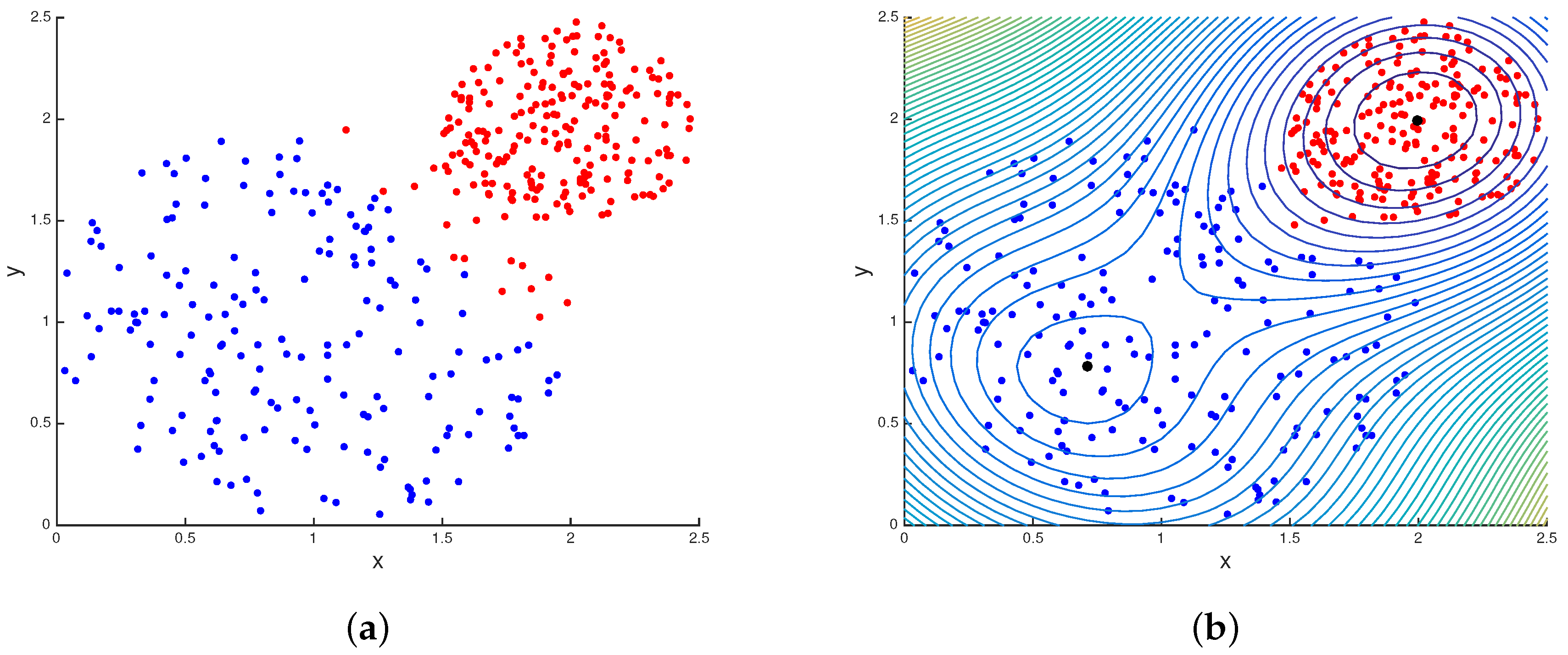
Figure 3.
Identification of four classes by quantum clustering.

Figure 4.
Center of disease potential.
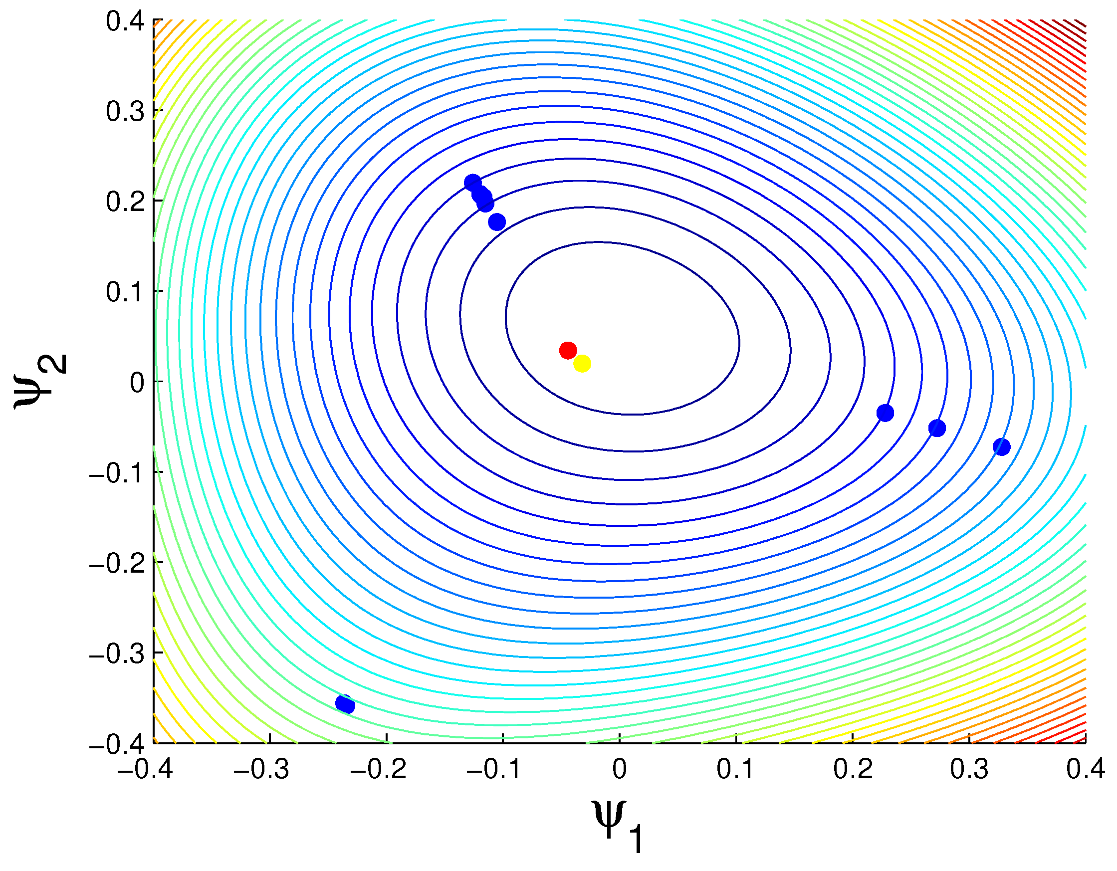
Figure 5.
A.Strehl 1000 2D points. (a) ; (b) .

Figure 6.
Smith and Draper data. (a) Reproduction of P. 1425 of [49]; (b) Quantum Clustering (QC) .
Figure 6.
Smith and Draper data. (a) Reproduction of P. 1425 of [49]; (b) Quantum Clustering (QC) .

Figure 7.
QC clustering applied to exoplanet data.


| Dataset | Row Dim. | Col.Dim. | No. Non-Zero Entries | Time (s) | Time (s) |
|---|---|---|---|---|---|
| N | K | nz | Method | B Method | |
| Bill Mark | 94 | 10,695 | 33,693 | 0.010820 | 0.115671 |
| Reuters | 2742 | 12,209 | 129,793 | 0.054852 | 0.201204 |
| Enron | 55,365 | 121,415 | 7,989,058 | 1.765044 | 5.741161 |
| user60784 | 2478 | 492,947 | 2,329,810 | 0.462936 | 4.790335 |
© 2017 by the authors. Licensee MDPI, Basel, Switzerland. This article is an open access article distributed under the terms and conditions of the Creative Commons Attribution (CC BY) license ( http://creativecommons.org/licenses/by/4.0/).
Share and Cite
MDPI and ACS Style
Scott, T.C.; Therani, M.; Wang, X.M. Data Clustering with Quantum Mechanics. Mathematics 2017, 5, 5. https://doi.org/10.3390/math5010005
AMA Style
Scott TC, Therani M, Wang XM. Data Clustering with Quantum Mechanics. Mathematics. 2017; 5(1):5. https://doi.org/10.3390/math5010005
Chicago/Turabian StyleScott, Tony C., Madhusudan Therani, and Xing M. Wang. 2017. "Data Clustering with Quantum Mechanics" Mathematics 5, no. 1: 5. https://doi.org/10.3390/math5010005
Note that from the first issue of 2016, this journal uses article numbers instead of page numbers. See further details here.