Analysis of Magneto-hydrodynamics Flow and Heat Transfer of a Viscoelastic Fluid through Porous Medium in Wire Coating Analysis

 ,
,  , and
, and
Abstract
:1. Introduction
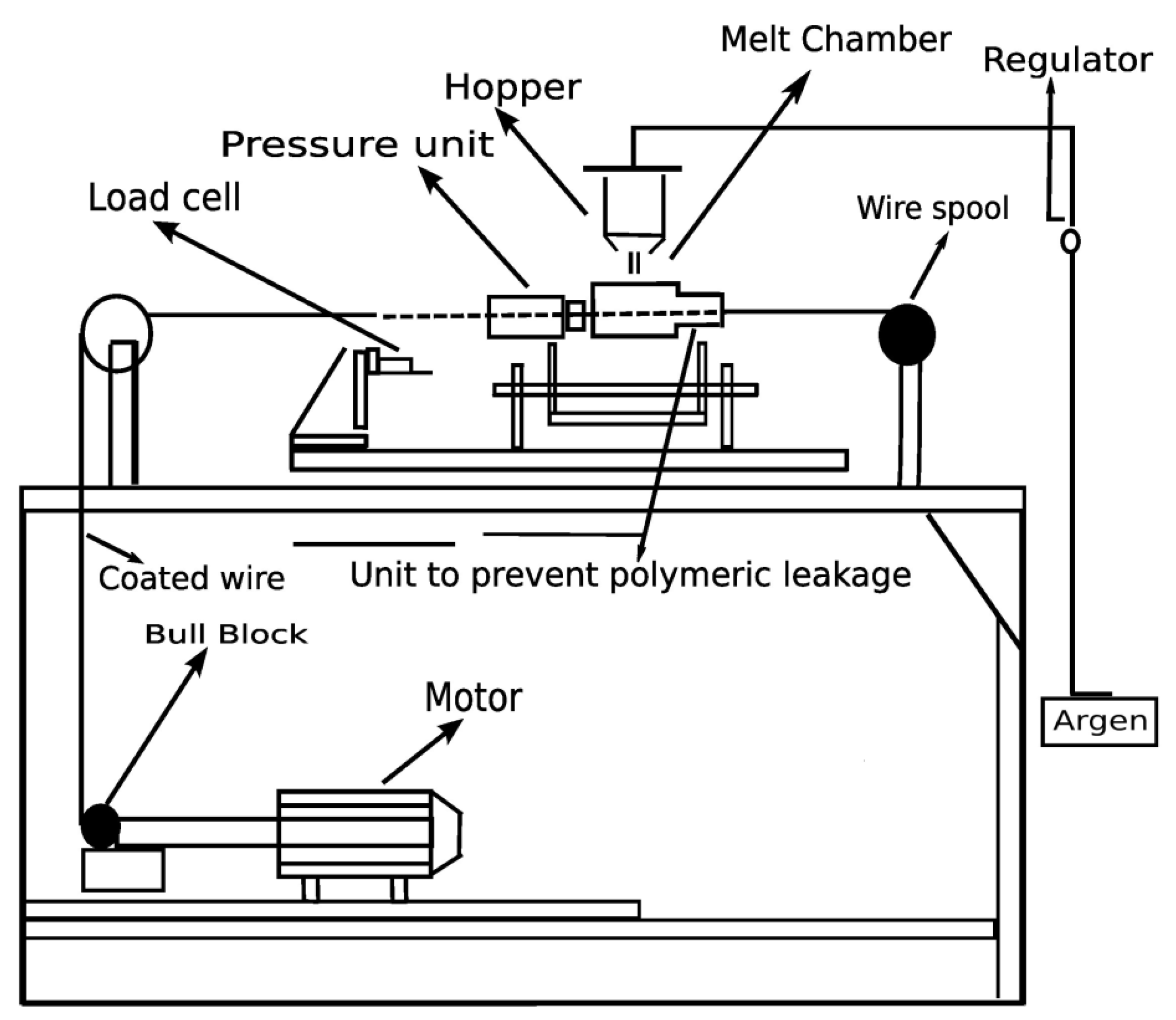
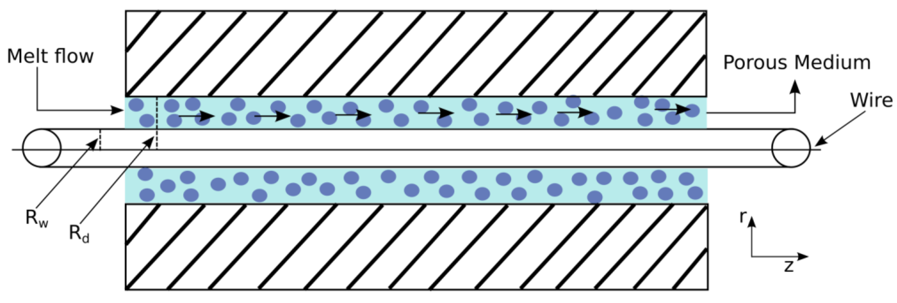
2. Modeling of the Problem
3. Solution by Homotopy Asymptotic Method
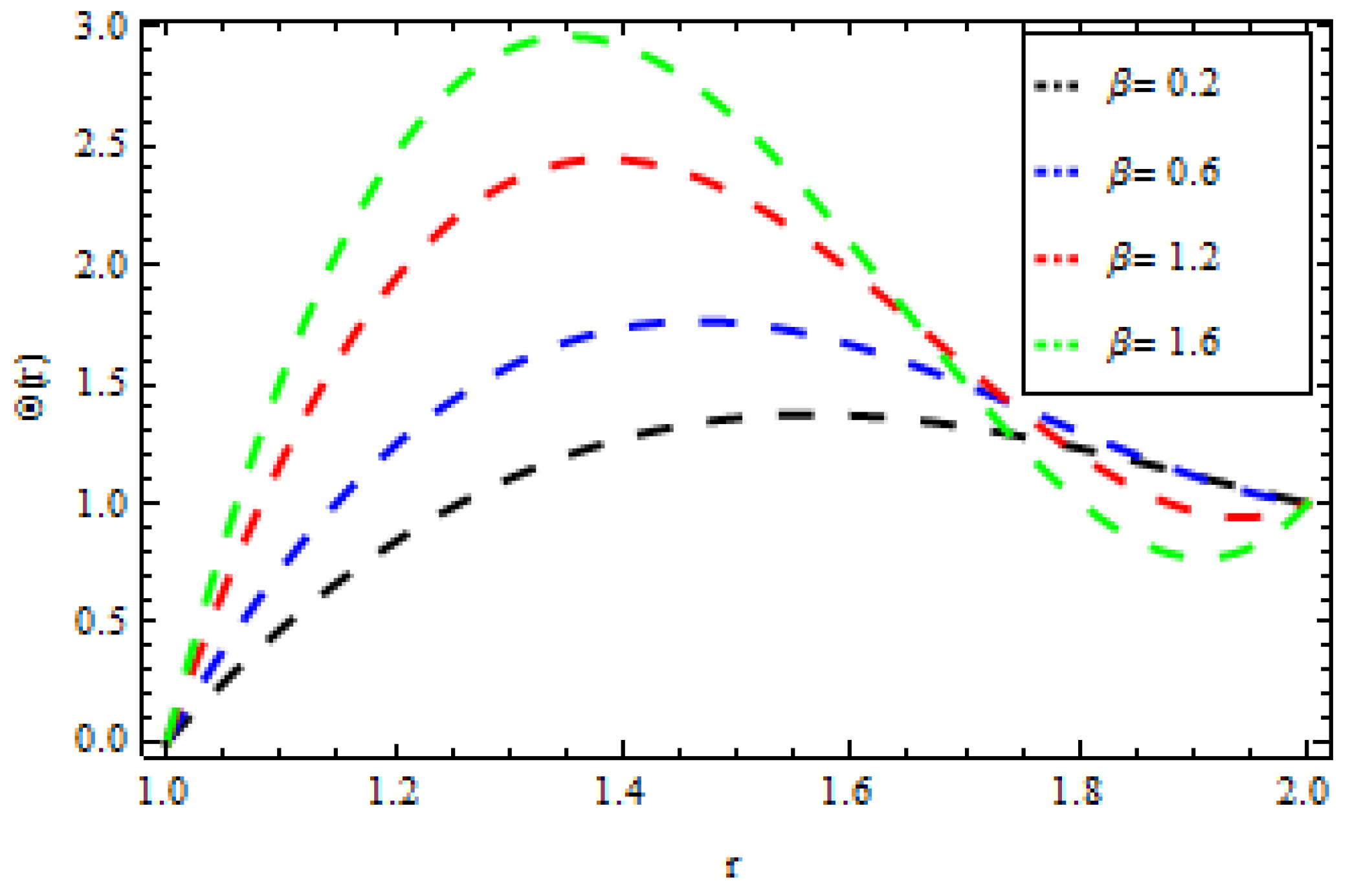
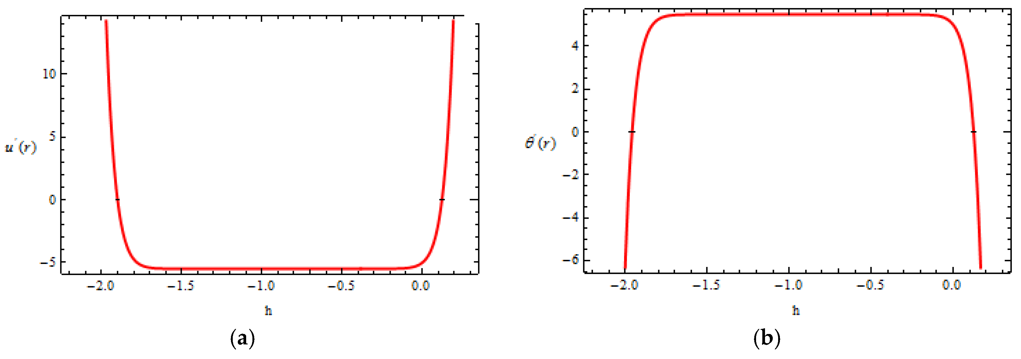
4. Results and Discussion
5. Conclusions
Author Contributions
Conflicts of Interest
References
- Han, C.D.; Rao, D. The rheology of wire coating extrusion. Polym. Eng. Sci. 1978, 18, 1019–1029. [Google Scholar] [CrossRef]
- Nayak, M.K. Wire Coating Analysis, 2nd ed.; India Tech: New Delhi, Indina, 2015. [Google Scholar]
- Caswell, B.; Tanner, R.J. Wire coating die using finite element methods. Polym. Eng. Sci. 1978, 18, 417–421. [Google Scholar] [CrossRef]
- Tucker, C.L. Computer Modeling for Polymer Processing; Hanser: Munich, Germany, 1989; pp. 311–317. [Google Scholar]
- Akter, S.; Hashmi, M.S.J. Analysis of polymer flow in a canonical coating unit: Power law approach. Prog. Org. Coat. 1999, 37, 15–22. [Google Scholar] [CrossRef]
- Akter, S.; Hashmi, M.S.J. Plasto-hydrodynamic pressure distribution in a tepered geometry wire coating unit. In Proceedings of the 14th Conference of the Irish manufacturing committee (IMC14), Dublin, Ireland, 3–5 September 1997; pp. 331–340. [Google Scholar]
- Siddiqui, A.M.; Haroon, T.; Khan, H. Wire coating extrusion in a Pressure-type Die in the flow of a third grade fluid. Int. J. Non-Linear Sci. Numeric. Simul. 2009, 10, 247–257. [Google Scholar]
- Fenner, R.T.; Williams, J.G. Analytical methods of wire coating die design. Trans. Plast. Inst. 1967, 35, 701–706. [Google Scholar]
- Shah, R.A.; Islam, S.; Siddiqui, A.M.; Haroon, T. Optimal homotopy asymptotic method solution of unsteady second grade fluid in wire coating analysis. J. Ksiam 2011, 15, 201–222. [Google Scholar]
- Shah, R.A.; Islam, S.; Siddiqui, A.M.; Haroon, T. Exact solution of differential equation arising in the wire coating analysis of an unsteady second grad fluid. Math. Comp. Mod. 2013, 57, 1284–1288. [Google Scholar] [CrossRef]
- Mitsoulis, E. Fluid flow and heat transfer in wire coating. Adv. Polym. Technol. 1986, 6, 467–487. [Google Scholar] [CrossRef]
- Oliveira, P.J.; Pinho, F.T. Analytical solution for fully developed channel and pipe flow of Phan-Thien, Tanner fluids. J. Fluid Mech. 1999, 387, 271–280. [Google Scholar] [CrossRef]
- Thien, N.P.; Tanner, R.I. A new constitutive equation derived from network theory. J. Non-Newtonian Fluid Mech. 1977, 2, 353–365. [Google Scholar] [CrossRef]
- Kasajima, M.; Ito, K. Post-treatment of Polymer extrudate in wire coating. Appl. Polym. Symp. 1973, 20, 221–235. [Google Scholar]
- Wagner, R.; Mitsoulis, E. Effect of die design on the analysis of wire coating. Adv. Polym. Technol. 1985, 5, 305–325. [Google Scholar] [CrossRef]
- Bagley, E.B.; Storey, S.H. Wire and wire ccoating product. Int. J. Polym. Sci. 1963, 38, 1104–1122. [Google Scholar]
- Pinho, F.T.; Oliveira, P.J. Analysis of forced convection in pipes and channels with simplified Phan-Thien-Tanner fluid. Int. J. Heat Mass Transf. 2000, 43, 2273–2287. [Google Scholar] [CrossRef]
- Shah, R.A.; Islam, S.; Siddiqui, A.M.; Haroon, T. Wire coating analysis with Oldroyd 8-constant fluid by optimal homotopy asymptotic method. Comput. Math. Appl. 2012, 63, 695–707. [Google Scholar] [CrossRef]
- Abel, S.; Prasad, K.V.; Mahaboob, A. Buoyancy force and thermal radiation effects in MHD boundary layer viscoelastic fluid flow over continuously moving stretching surface. Int. J. Therm. Sci. 2005, 44, 465–476. [Google Scholar] [CrossRef]
- Sarpakaya, T. Flow of non-Newtonian fluids in a magnetic field. AIChE J. 1961, 7, 324–328. [Google Scholar] [CrossRef]
- Abel, M.S.; Shinde, J.N. The effects of MHD flow and heat transfer for the UCM fluid over a stretching surface in presence of thermal radiation. Adv. Math. Phys. 2015, 2012, 21. [Google Scholar] [CrossRef]
- Chen, V.C. On the analytical solution of MHD flow and heat transfer for two types of viscoelastic fluid over a stretching sheet with energy dissipation, internal heat source and thermal radiation. Int. J. Heat Mass Transf. 2010, 19, 4264–4273. [Google Scholar] [CrossRef]
- Hayat, T.; Sajid, M. Homotopy analysis of MHD boundary layer flow of an upper-convected Maxwell fluid. Int. J. Eng. Sci. 2007, 45, 393–401. [Google Scholar] [CrossRef]
- Wang, Y.; Hayat, T. Fluctuating flow of a Maxwell fluid past a porous plate with variable suction, Nonlinear Analysis. Real World Appl. 2008, 9, 1269–1282. [Google Scholar] [CrossRef]
- Rashidi, S.; Dehghan, M. Study of stream wise transverse magnetic fluid flow with heat transfer around an obstacle embedded in a porous medium. J. Magn. Magn. Mater. 2015, 378, 128–137. [Google Scholar] [CrossRef]
- Ellahi, R.; Rahman, S.U.; Nadeem, S.; Vafai, K. The blood flow of Prandtl fluid through a tapered stenosed arteries in permeable walls with magnetic field. Commun. Theor. Phys. 2015, 63, 353–358. [Google Scholar] [CrossRef]
- Kandelousi, M.S.; Ellahi, R. Simulation of ferrofluid flow for magnetic drug targeting using the lattice Boltzmann method. Z. Naturf. A 2015, 70, 115–124. [Google Scholar] [CrossRef]
- Nayak, M.K. Chemical reaction effect on MHD viscoelastic fluid over a stretching sheet through porous medium. Mecanica 2016, 51, 1699–1711. [Google Scholar] [CrossRef]
- Vafai, K. Handbook of Porous Media, 2nd ed.; Taylor and Francis: New York, NY, USA, 2015. [Google Scholar]
- Nield, I.A.; Bejan, A. Cpvection in Porou Media, 4th ed.; Springer: New York, NY, USA, 2012. [Google Scholar]
- Daniel, Y.S. Steady MHD laminar flows and heat transfer adjacent to porous stretching sheet using HAM. Am. J. Heat Mass Transf. 2015, 2, 146–159. [Google Scholar] [CrossRef]
- Nayak, M.K. Flow through Porous Median, 1st ed.; India Tech: New Delhi, India, 1989. [Google Scholar]
- Liao, S.J. An analytic solution of unsteady boundary layer flows caused by an impulsively stretching plate. Commun. Nonlinear Sci. Numer Simul. 2006, 11, 326–339. [Google Scholar] [CrossRef]
- Liao, S.J. A new branch of solutions of boundary layer flows over a permeable stretching plate. Int. J. Nonlinear Mech. 2007, 42, 819–830. [Google Scholar] [CrossRef]
- Liao, S.J. Beyond perturbation: review on the basic ideas of homotopy analysis method and its application. Adv. Mech. 2008, 38, 1–34. [Google Scholar]
- Abbasbandy, S. The application of homotopy analysis method to nonlinear equations arising in heat transfer. Phys. Lett. A 2006, 360, 109–113. [Google Scholar] [CrossRef]
- Abbasbandy, S. Homotopy analysis method for heat radiation equation. Int. Commun. Heat Mass Transf. 2007, 34, 380–387. [Google Scholar] [CrossRef]
- Hayat, T.; Khan, M.; Ayub, M. On the explicit analytic solutions of an Oldroyd 6-constant fluid. Int. J. Eng. Sci. 2004, 42, 123–135. [Google Scholar] [CrossRef]
- Hayat, T.; Khan, M.; Asghar, S. Homotopy analysis of MHD flows of an Oldroyd 6-constant fluid. Acta Mech. 2004, 168, 213–232. [Google Scholar] [CrossRef]
- Khan, M.; Abbas, Z.; Hayat, T. Analytic solution for the flow of Sisko fluid through a porous medium. Transp. Porous Media 2008, 71, 23–37. [Google Scholar] [CrossRef]
- Abbas, Z.; Sajid, M.; Hayat, T. MHD boundary layer flow of an upper-convected Maxwell fluid in porous channel. Theor. Comput. Fluid Dyn. 2006, 20, 229–238. [Google Scholar] [CrossRef]
- Khan, W.; Gul, T.; Idrees, M.; Islam, S.; Khan, I.; Dennis, L.C.C. Thin Film Williamson Nanofluid Flow with Varying Viscosity and Thermal Conductivity on a Time-Dependent Stretching Sheet. Appl. Sci. 2016, 6. [Google Scholar] [CrossRef]


| r | ||
|---|---|---|
| [2/2] | −0.451024 | −0.654021 |
| [3/3] | −0.452521 | −0.653145 |
| [4/4] | −0.452365 | −0.653541 |
| [5/5] | −0.452630 | −0.653640 |
| [6/6] | −0.452315 | −0.654612 |
| [7/7] | −0.452001 | −0.654441 |
| r | ||
|---|---|---|
| [2/2] | −0.7624392 | −0.663219 |
| [3/3] | −0.7621111 | −0.6639111 |
| [4/4] | −0.7636667 | −0.6646667 |
| [5/5] | −0.7633333 | −0.6645953 |
| [6/6] | −0.7621012 | −0.6634444 |
| [7/7] | −0.7621142 | −0.6633568 |
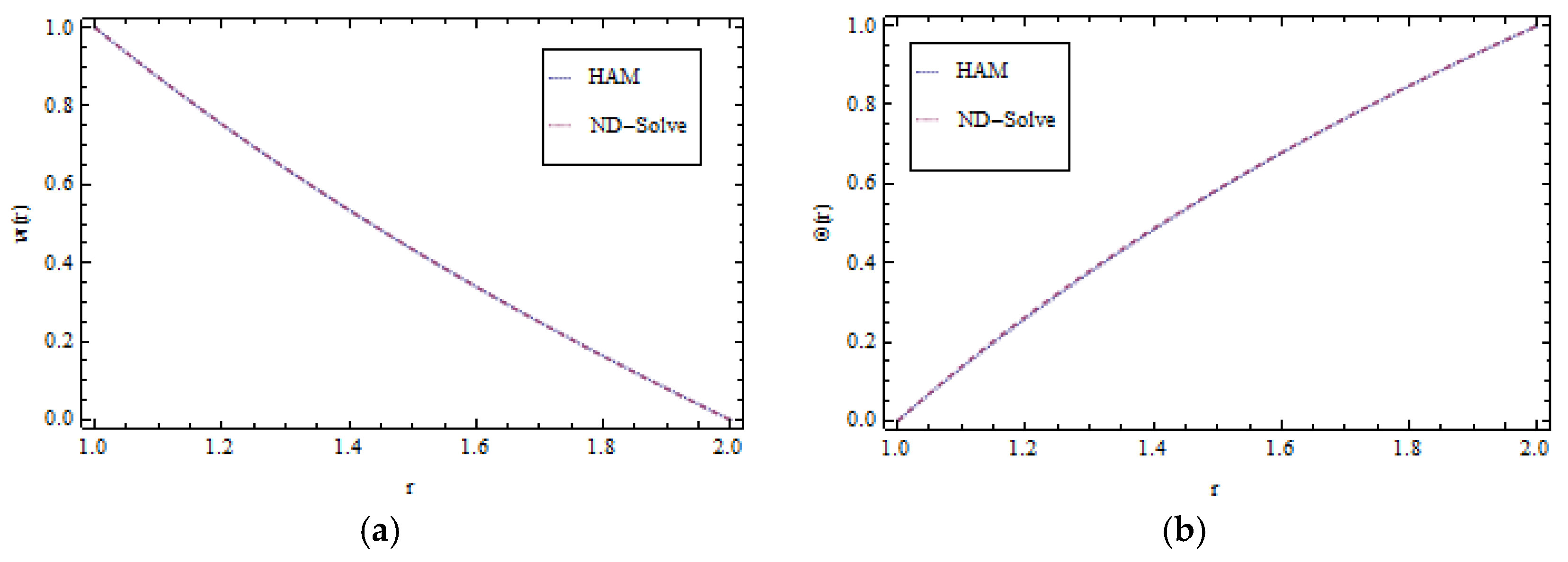
| r | HAM | ND-Solve | ADM | Relative Error of HAM and ND-Solve |
|---|---|---|---|---|
| 1.0 | 1 | 1 | 1 | 0 |
| 1.2 | 0.66070791111 | 0.66070791111 | 0.66070791123 | 2.3 |
| 1.4 | 0.41585866667 | 0.41585866667 | 0.41585866665 | 6.7 |
| 1.6 | 0.23559573333 | 0.23559573333 | 0.23559573322 | 0.2 |
| 1.8 | 0.10125404444 | 0.10125404444 | 0.10125404443 | 0.3 |
| 2.0 | 0 | 1.17763568 | 1.015426227 | 0.012 |
© 2017 by the authors. Licensee MDPI, Basel, Switzerland. This article is an open access article distributed under the terms and conditions of the Creative Commons Attribution (CC BY) license (http://creativecommons.org/licenses/by/4.0/).
Share and Cite
Khan, Z.; Khan, M.A.; Islam, S.; Jan, B.; Hussain, F.; Ur Rasheed, H.; Khan, W. Analysis of Magneto-hydrodynamics Flow and Heat Transfer of a Viscoelastic Fluid through Porous Medium in Wire Coating Analysis. Mathematics 2017, 5, 27. https://doi.org/10.3390/math5020027
Khan Z, Khan MA, Islam S, Jan B, Hussain F, Ur Rasheed H, Khan W. Analysis of Magneto-hydrodynamics Flow and Heat Transfer of a Viscoelastic Fluid through Porous Medium in Wire Coating Analysis. Mathematics. 2017; 5(2):27. https://doi.org/10.3390/math5020027
Chicago/Turabian StyleKhan, Zeeshan, Muhammad Altaf Khan, Saeed Islam, Bilal Jan, Fawad Hussain, Haroon Ur Rasheed, and Waris Khan. 2017. "Analysis of Magneto-hydrodynamics Flow and Heat Transfer of a Viscoelastic Fluid through Porous Medium in Wire Coating Analysis" Mathematics 5, no. 2: 27. https://doi.org/10.3390/math5020027