
An Analysis on the Fractional Asset Flow Differential Equations


1
Department of Mathematics, Faculty of Science, Mahidol University, Bangkok 10400, Thailand
2
Centre of Excellence in Mathematics, Commission on Higher Education, Ministry of Education, Si Ayutthaya Road, Bangkok 10400, Thailand
3
Department of Mathematics, Faculty of Applied Science, King Mongkut’s University of Technology North Bangkok, Bangkok 10800, Thailand
*
Author to whom correspondence should be addressed.
Mathematics 2017, 5(2), 33; https://doi.org/10.3390/math5020033
Submission received: 30 March 2017
/
Revised: 9 June 2017
/
Accepted: 12 June 2017
/
Published: 16 June 2017
(This article belongs to the Special Issue Recent Developments in the Theory and Applications of Fractional Calculus)
Abstract
:The asset flow differential equation (AFDE) is the mathematical model that plays an essential role for planning to predict the financial behavior in the market. In this paper, we introduce the fractional asset flow differential equations (FAFDEs) based on the Liouville-Caputo derivative. We prove the existence and uniqueness of a solution for the FAFDEs. Furthermore, the stability analysis of the model is investigated and the numerical simulation is accordingly performed to support the proposed model.
1. Introduction
In recent years, the important thing for financial behavior has been understanding and classifying the dynamics of the financial system such as price crashes, bubbles, momentum and liquidity. Over the last three decades, the mathematical model has played an essential role in preparing planning to predict the financial behavior in the market in the future. Thus, a number of mathematical models have been used to predict financial behavior [1,2,3,4,5,6,7,8,9,10,11,12]. Moreover, in order to obtain better simulation of future phenomena, nonlinear continuous models have also developed. Researchers proposed several nonlinear continuous models for describing the complicated dynamics of the financial system. For example, in 2008, Fanti et al. [10] proposed the behavior of capital stock by using a dynamic Investment Saving-Liquidity Preference Money Supply (IS-LM) model with delay, and Chatterjee et al. [11] proposed a dynamic Hecker-Ohlin model and considered the equilibrium of the model. Moreover, Yang et al. [12] proposed a herd mechanism of an open financial market for considering volatility and parameters of bubbles and collapses in the market. In this paper, we study the analysis of a nonlinear system that is the asset flow differential equations (AFDEs). AFDEs were proposed and developed by Gaginalp et al. [13]. They investigated the solution of autonomous equations with dimension . This model may describe many behaviors in real financial markets [13,14,15,16]. The model variables are explained by the demand, the supply, the market price, the transition rate, the trend-based and value-based of the investor preferences at sudden times [13,17,18].
Fractional calculus was introduced for over three centuries. At the beginning, fractional calculus was only in a theoretical sense. The traditional system of integer-order of differential equations may fail to explain complicated incidents in real phenomena. However, nowadays, fractional order of differential equations has been applied to model the complicated real situations involving many areas—for example, physics, engineering, epidemic, finance and sciences [19,20,21,22,23,24]. The concept of a fractional model helps with expressing the data structure for real life situations more than the integer model. The main dominant point of fractional order equations compared to integer order equations is its memory, which is the history of the system [25,26,27].
Since variables in the financial system have long memories, the fractional order system is suitable for studying the behavior in financial systems. There are many papers proposing fractional-order differential equations for the financial system [25,26,27,28] consisting of the parts of products, money, bond and labor force. Here, we propose a system of time-fractional differential equations modified from the Gaginalp’s model [13] to describe the behavior of asset flow in the financial market.
A number of researchers studied about the existence and uniqueness for the solution of fractional differential equations [29,30,31,32,33,34]. However, there has been a lack of research focusing on the global existence and uniqueness for the solution of the fractional asset flow differential equations (FAFDEs). In this paper, we propose an alternative way to prove the local existence solution of the system of fractional-order differential equations by the Banach fixed point theorem, which helps to explain the solution of the fractional model. Moreover, the global existence for the solution of the fractional model can be express by continuation theorem.
The remainder of this work is organized as follows. In Section 2, the definitions and lemma involving the fractional-order differential equations are presented. In addition, we present the fractional-order model in this section. In Section 3, the local existence and uniqueness theorem of the model’s solution is presented. In Section 4, we propose the continuation theorems for the model to extend the local solution into the global solution. The stability analysis of the fractional model is presented and is followed by the numerical simulation in Section 6. Finally, Section 7 concludes and discusses this work.
2. Model Formulation
2.1. Fractional Calculus
Definition 1.
The Riemann–Liouville integral of order for a function f is defined as:
where Γ is the gamma function.
Definition 2.
The Riemann–Liouville derivative of order for a function is defined as:
The regularization definition of the Riemann–Liouville derivative was introduced by Liouville–Caputo in 1967 [36].
Definition 3.
The Liouville–Caputo–type fractional derivative of order for a function is defined by:
The most regular definition is the Liouville–Caputo-type definition because the initial condition for fractional order differential equations with Liouville–Caputo-type derivatives is similar in form to the integer-order differential equation [19,20,21,22].
Lemma 1.
(Banach fixed point theorem) Let A be a closed convex bounded subset of a Banach space X and V be a contraction mapping from A into A. Then, there exists a unique such that .
2.2. Fractional Model
The behavior of price dynamic in the market based on:
| the market price of an asset at time t, | |
| the fraction of total asset invested in the stock at time t, | |
| the trend-based component of the investor preference at time t, | |
| the value-based component of the investor preference at time t, | |
| the fundamental value, | |
| D | the demand, |
| S | the supply. |
Gaginalp et al. [13] proposed the dynamical system of AFDEs to describe those four state variables in the market price :
where and are positive constants for .
The value of the market price of an asset at time t can be only a positive number and cannot be approached to infinity, the value of the fraction of total assets is defined between 0 and 1. The demand and the supply can be determined as and , respectively. is the transition rate that is dependent on and defined by , is an increasing continuous function with , and and are positive constants.
In this article, the FAFDEs based on the Liouville–Caputo fractional derivative are introduced as follows:
where is the Liouville–Caputo fractional derivative of order , are positive constants for and are positive constants for
We need the following assumptions; let X be a Banach space with its norm .
- (A1)
- is increasing and continuously differentiable where , and satisfies that for anyfor some positive constant .
- (A2)
- is continuous and satisfies there being two constants and such that:and for any .
- (A3)
- is continuously differentiable and has the following: there exists two positive constants and such that:and for any .
3. Local Existence and Uniqueness of a Solution
In this section, we show that system (5) has a unique continuous solution by the Banach fixed point theorem. To do so, we introduce a Banach space:
and its norm is defined by:
with T being a positive constant.
Theorem 1.
Proof.
Let M be a constant with .
Choose a positive constant h where:
Let with . Then, is a Banach space equipped with the norm for any .
We construct the set . Clearly, is closed, bounded and convex.
We also define the operator by where with and are given by:
Let . We want to show that
Consider
Consider
By the inequality (6),
Consider
Then,
Consider
Then,
Then, this means that B maps U into itself.
Next, we want to show that B is a contraction mapping.
Consider
where .
Thus,
Consider
where .
Thus,
Consider
where .
Thus,
Consider
where .
Thus,
We have that from the inequalities (11)–(14) and the definition of h as in the inequality (6):
with . This shows that B is a contraction mapping.
Therefore, by Banach fixed point theorem, system (5) has a unique continuous solution on ☐
4. Continuation Theorems
In this section, we extend the continuation theorem for the system of FAFDEs. Firstly, we give the following lemma.
Lemma 2.
(Gronwall-Bellman inequality [37]) Suppose , is a nonnegative function that is locally integrable on , and is a nonnegative, nondecreasing continuous bounded function defined on . If is nonnegative and locally integrable on with:
on this interval, then:
Furthermore, if is nondecreasing on then:
where is the Mittag–Leffler function defined by:
Theorem 2.
Proof.
Suppose that solution of system (5) has the maximal existence interval defined by with . Let us consider: for
By the assumption of theorem, is bounded on , we have that for and then for ,
It follows from the Lemma 2 that, for ,
It is well-known that the is an analytic function [38] and then we can conclude the is bounded on .
Next, we consider on . Then, for ,
Since and are bounded on such that . Then;
By Lemma 2, we obtain:
Thus, is bounded on Hence, is bounded on . Since x are continuous and bounded on , is finite.
Let with . Then,
Consider Let
Similar to Theorem 1, we can construct the positive constant depending on and such that our problem has a solution on . This part is shown in the below.
Let be a Banach space with the norm and . Then, is a Banach space equipped with the norm for any .
We construct the set .
We define the operator by for and for any , is constructed by:
where ,
and ,
and ,
and .
To make it clear about the construction of , without loss of generality, we only show that maps into . Let us consider that for :
In this case, the constant is determined by:
We can construct in this way and follow method as in Theorem 1.
By considering as the Theorem 1, has a fixed point , that is for . We next define the function on by:
We can see that is a continuous solution of our problem on with
We thus get a contradiction. Therefore, system (5) has a solution on . ☐
Remark 1.
Because and are the market price and the fraction of total asset invested, respectively. By assumptions of the model [13], it is possible to assume that and are bounded.
5. Stability Analysis
In order to determine the stability of system (5), we firstly consider the equilibrium point. To find the equilibrium point we set all equations of system (5) to zero:
Then:
where:
where:
where:
with and for .
The characteristic equation of for is:
where:
Proposition 1.
The equilibrium points are locally asymptotically stable if all the eigenvalues λ of the Jacobian matrix evaluated at the equilibrium points satisfy:
Theorem 3.
If and , then the equilibrium point is locally asymptotically stable.
Proof.
From the equations (18) and (19), we can find eigenvalues of the Jacobian matrix corresponding to the equilibrium points from the fourth-order characteristic equation. Under assumptions of this theorem, Ahmed et al. [41] show that for all eigenvalues λ. From Proposition 1, we can conclude that the equilibrium points of system (5) is locally asymptotically stable. ☐
6. Numerical Simulation
The exact solution of some fractional order differential equations can not be found. Thus, the numerical solutions for fractional order differential equation model (5) can be approached by using an algorithm based on an Adams–Bashforth type predictor-corrector method [42,43].
The numerical solutions of system (5) are carried out by setting functions and . The model parameters are chosen to be and , with the initial conditions and
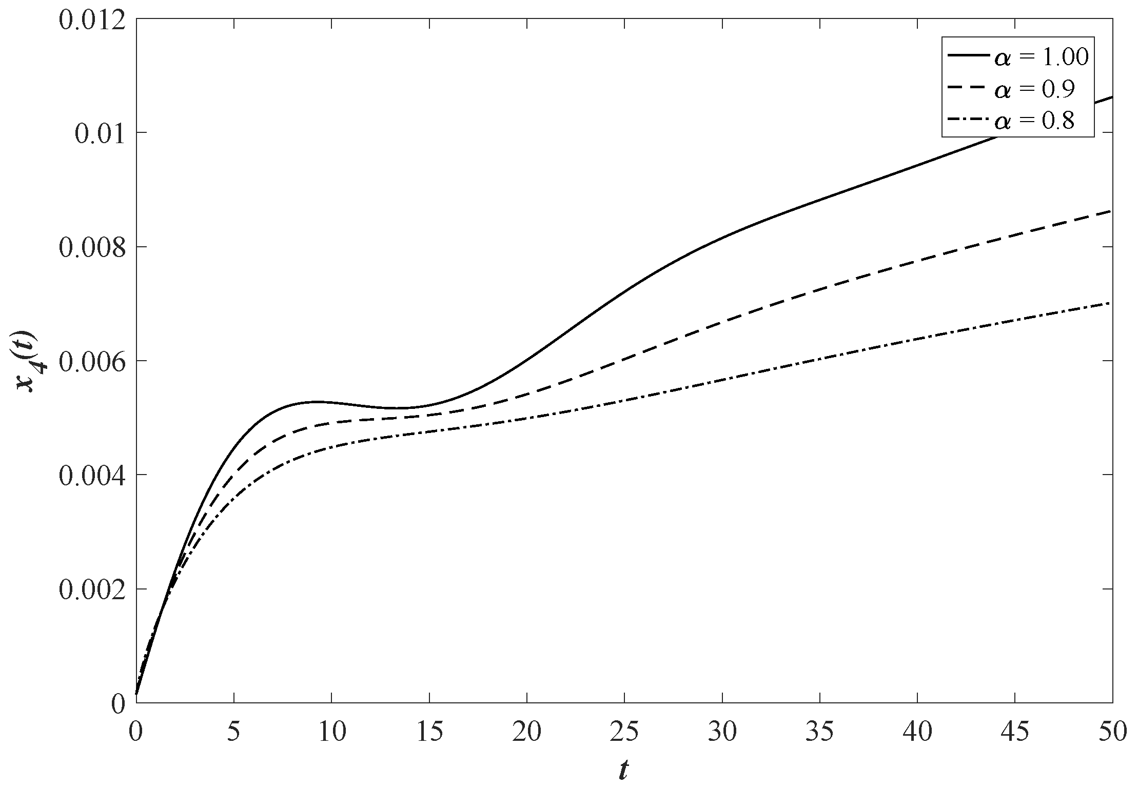
The approximate solutions of market price , fraction of total asset , trend-based component and value-based component of the FAFDEs with the different values of order, and are shown in Figure 1, Figure 2, Figure 3 and Figure 4, respectively.
The results in Figure 1, Figure 2 and Figure 3 indicate that the behavior for the market price of an asset, the fraction of total asset invested in the stock, and the trend-based component of the investor preference have the same pattern at each time for an integer–order system with and a fractional–order system with and . To investigate the effect of fractional derivative order on market behavior, the numerical results demonstrate that a decrease in the derivative order is associated with a decrease in the maximum value of and . Figure 4 shows that decreasing of derivative order leads to a decrease in the value-based component at each time. In addition, the market price as shown in Figure 1 represents the pattern of head and shoulders or rounding top, in which a major high appears by a local maximum. In order to execute planning in the future, investors can buy or sell when the pattern completes. By Theorem 3, the equilibrium point is locally stable, where and In other words, the values of and converge to equilibrium point at some long-term behaviors.
7. Discussion and Conclusions
In this paper, we have proposed a fractional order asset flow differential equations model, which is a generalization of an integer order model proposed by Gaginalp [13]. Then, we propose and prove the local existence and uniqueness theorems for the solution of the model by applying the Banach fixed point theorem. After that, we extend the local solution, to a global solution, by proposing the continuation theorem for the model. The stability of the model is also investigated and we obtain the sufficient condition of the parameters. The numerical solutions of the model are illustrated by using an Adams–Bashforth type predictor-corrector method.
Acknowledgments
This research was funded by King Mongkut’s University of Technology North Bangkok, contract no. KMUTMB-GEN-55-16. Appreciation is extended to Faculty of Science, Mahidol University, Bangkok, Thailand.
Author Contributions
Din Prathumwan and Panumart Sawangtong developed the mathematical model. Wannika Sawangtong and Panumart Sawangtong proposed the research idea for proving theorems. Wannika Sawangtong and Din Prathumwan were responsible for simulating the results by the MATLAB programming. Din Prathumwan wrote this paper. All authors contributed in editing and revising the manuscript.
Conflicts of Interest
The authors declare no conflict of interest.
References
- Ma, J.H.; Chen, Y.S. Study for the bifurcation topological structure and the global complicated character of a kind of nonlinear finance system—I. Appl. Math. Mech. 2001, 22, 1240–1251. [Google Scholar]
- Ma, J.H.; Chen, Y.S. Study for the bifurcation topological structure and the global complicated character of a kind of nonlinear finance system—II. Appl. Math. Mech. 2001, 22, 1375–1382. [Google Scholar]
- Cesare, L.D.; Sportelli, M. A dynamic IS-LM model with delayed taxation revenues. Chaos Solitons Fractals 2005, 25, 233–244. [Google Scholar]
- Fanti, L.; Manfredi, P. Chaotic business cycles and fiscal policy: An IS-LM model with distributed tax collection lags. Chaos Solitons Fractals 2007, 32, 736–744. [Google Scholar]
- Frisch, R.; Holme, H. The Characteristic Solutions of a Mixed Difference and Differential Equation Occuring in Economic Dynamics. Econometrica 1935, 3, 225–239. [Google Scholar]
- He, X.Z.; Li, K.; Wei, J.; Zheng, M. Market stability switches in a continuous-time financial market with heterogeneous beliefs. Econ. Model. 2009, 26, 1432–1442. [Google Scholar]
- Chiarella, C.; Dieci, R.; Gardini, L. Asset price dynamics in a financial market with fundamentalists and chartists. Discret. Dyn. Nat. Soc. 2001, 2, 69–99. [Google Scholar]
- He, X.Z.; Zheng, M. Dynamics of moving average rules in a continuous-time financial market model. J. Econ. Behav. Organ. 2010, 76, 615–634. [Google Scholar]
- Chiarella, C.; He, X.Z.; Zheng, M. An analysis of the effect of noise in a heterogeneous agent financial market model. J. Econ. Dyn. Control 2011, 35, 148–162. [Google Scholar]
- Zhou, L.; Li, Y. A generalized dynamic IS-LM model with delayed time in investment processes. Appl. Math. Comput. 2008, 196, 774–781. [Google Scholar]
- Chatterjee, P.; Shukayev, M. A stochastic dynamic model of trade and growth: Convergence and diversification. J. Econ. Dyn. Control 2012, 36, 416–432. [Google Scholar]
- Yang, H.; Li, L.; Wang, D. Research on the stability of open financial system. Entropy 2015, 17, 1734–1754. [Google Scholar]
- Caginalp, G.; Balenovich, D. Asset flow and momentum: Deterministic and stochastic equations. Philos. Trans. R. Soc. 1999, 357, 2119–2133. [Google Scholar]
- Caginalp, G.; Ermentrout, G.B. A kinetic thermodynamics approach to the psychology of dluctuations in financial market. Appl. Math. Lett. 1990, 3, 17–19. [Google Scholar]
- Merdan, H.; Alisen, M. A mathematical model for asset pricing. Appl. Math. Comput. 2011, 218, 1449–1456. [Google Scholar]
- Sullivan, A.; Sheffrin, S.M. Economics: Principles in Action; Prentice Hall: Upper Saddle River, NJ, USA, 2005. [Google Scholar]
- Caginalp, G.; Balenovich, D. Market oscillations induced by the competition between value-based and trend-based investment strategies. Appl. Math. Financ. 1994, 1, 129–164. [Google Scholar]
- Caginalp, G.; Ermentrout, B. Numerical studies of differential equations related to theoretical financial markets. Appl. Math. Lett. 1991, 4, 35–38. [Google Scholar]
- Podlubny, I. Fractional Differential Equations. Mathematics in Science and Engineering; Academic Press: San Diego, CA, USA, 1999; Volume 198. [Google Scholar]
- Area, I.; Batarfi, H.; Losada, J.; Nieto, J.J.; Shammakh, W.; Torres, A. On a fractional order Ebola epidemic model. Adv. Differ. Equ. 2015, 2015, 278. [Google Scholar]
- Sofuoglu, Y.; Ozalp, N. A fractional rrder model on bilingualism. Commun. Fac. Sci. Univ. Ank. Ser. A 2014, 2014, 81–89. [Google Scholar]
- Sofuoglu, Y.; Ozalp, N. Fractional order bilingualism model without conversion from dominant unilingual group to bilingual group. Differ. Equ. Dyn. Syst. 2015, 2015, 1–9. [Google Scholar]
- Hilfer, R. Applications of Fractional Calculus in Physics; World Scientific: Hackensack, NJ, USA, 2001. [Google Scholar]
- Mainardi, F. Fractional relaxation-oscillation and fractional diffusion-wave phenomena. Chaos Solitons Fractals 1996, 7, 1461–1477. [Google Scholar]
- Dadras, S.; Momeni, H.R. Control of a fractional-order economical system via sliding mode. Phys. A Stat. Mech. Appl. 2010, 389, 2434–2442. [Google Scholar]
- Wang, Z.; Huang, X.; Shi, G. Analysis of nonlinear dynamics and chaos in a fractional order financial system with time delay. Comput. Math. Appl. 2011, 62, 1531–1539. [Google Scholar]
- Chen, W.C. Nonlinear dynamics and chaos in a fractional-order financial system. Chaos Solitons Fractals 2008, 36, 1305–1314. [Google Scholar]
- Li, Q.; Zhou, Y.; Zhao, X.; Ge, X. Fractional order stochastic differential equation with application in european option pricing. Discret. Dyn. Nat. Soc. 2014, 2014, 621895. [Google Scholar]
- Li, C.; Sarwar, S. Existence and contiuation of solution for Caputo type fractional differential equations. Electron. J. Differ. Equ. 2016, 2016, 1–14. [Google Scholar]
- Babakhani, D.; Gejji, V.D. Existence of positive solutions of nonlinear fractional differential equations. J. Math. Anal. Appl. 2003, 278, 434–442. [Google Scholar]
- Diethlm, K.; Ford, N.J. Analysis of fractional differential equations. J. Math. Anal. Appl. 2002, 265, 229–248. [Google Scholar]
- Yu, C.; Gao, G. Existence of fractional differential equations. J. Math. Anal. Appl. 2005, 310, 26–29. [Google Scholar]
- Kou, C.; Zhou, H.; Li, C.P. Existence and continuation theorems of fractional Riemann–Liouville type fractional differential equations. Int. J. Bifurc. Chaos 2012, 22, 1250077. [Google Scholar]
- Deng, W.H.; Li, C.P.; Guo, Q. Analysis of fractional differential equations with multi orders. Fractals 2007, 15, 173–182. [Google Scholar]
- Kilbas, A.A.; Srivastava, H.M.; Trujillo, J.J. Theory and Applications of Fractional Differential Equations; Elsevier Science: Amsterdam, The Netherlands, 2006. [Google Scholar]
- Caputo, M. Linear model of dissipation whose Q is almost frequency independent-II. Geophys. J. Int. 1967, 13, 529–539. [Google Scholar]
- Gronwall, T.H. Note on the derivatives with respect to a parameter of the solutions of a system of differential equations. Ann. Math. 1919, 20, 292–296. [Google Scholar]
- Gorenflo, R.; Kilbas, A.A.; Mainardi, F.; Rogosin, S.V. Mittag-Leffer Function, Related Topics and Applications; Springer: New York, NY, USA, 2014. [Google Scholar]
- Tavazoei, M.S.; Haeri, M. Unreliability of frequency-domain approximation in recognising chaos in fractional-order systems. IET Signal Proc. 2007, 1, 171–181. [Google Scholar]
- Petráš, I. Stability of fractional-order systems with rational orders: A survey. Fract. Calc. Appl. Anal. 2009, 12, 269–298. [Google Scholar]
- Ahmed, E.; El-Sayed, A.M.A.; El-Saka, H.A.A. On some Routh–Hurwitz conditions for fractional order differential equations and their applications in Lorenz, Rössler, Chua and Chen systems. Phys. Lett. A 2006, 358, 1–4. [Google Scholar]
- Diethelm, K.; Ford, N.J.; Freed, A.D. Detailed error analysis for a fractional Adams method. Numer. Algorithms 2004, 36, 31–52. [Google Scholar]
- Diethelm, K. An algorithm for the numerical solution of differential equations of fractional order. Electron. Trans. Numer. Anal. 1997, 5, 1–6. [Google Scholar]
Figure 1.
Market price for order and .
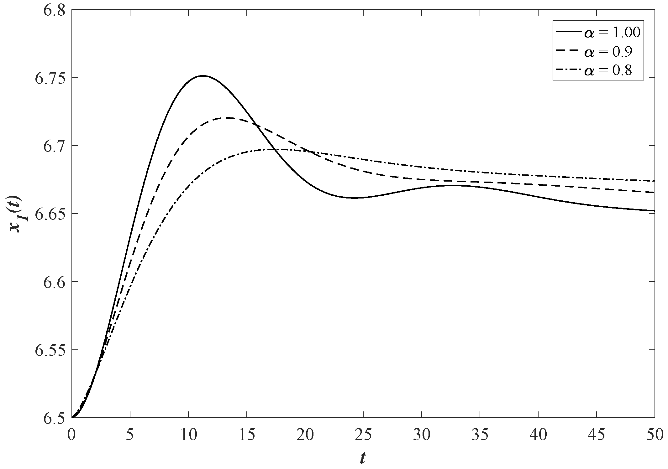
Figure 2.
Fraction of total asset for order and .
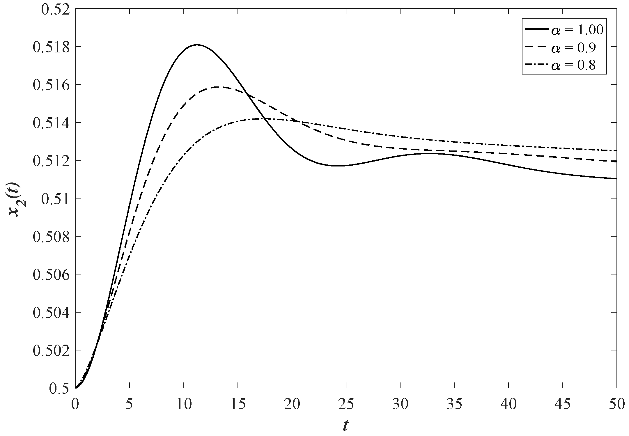
Figure 3.
Trend-based component for order and .
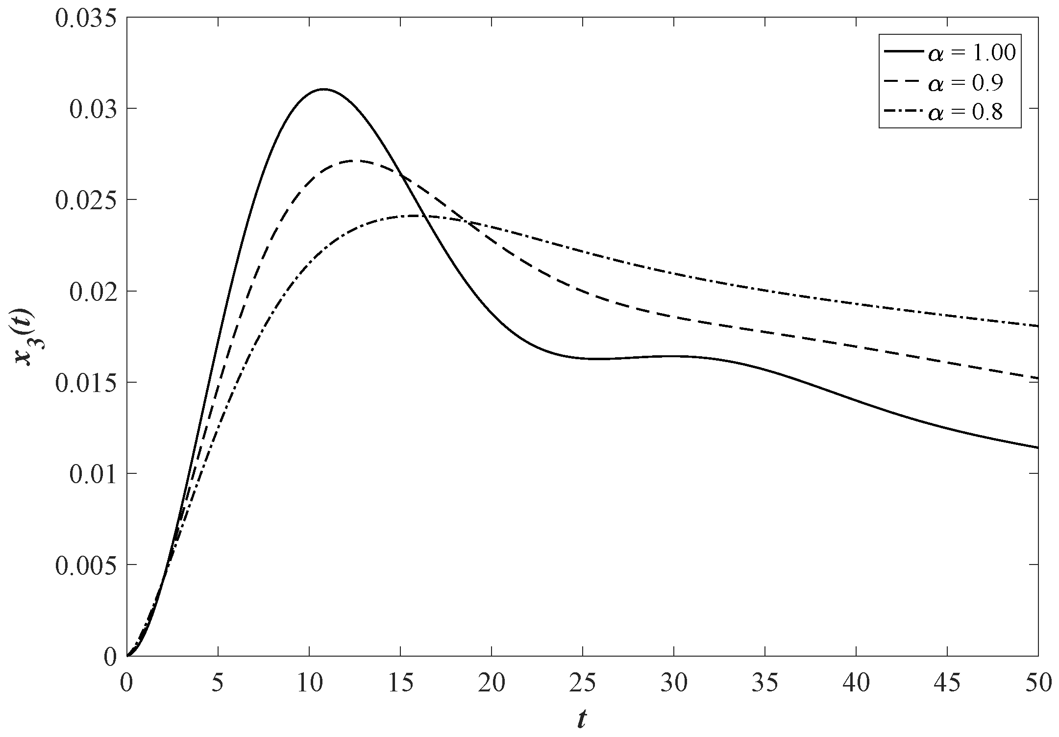
Figure 4.
Value-based component for order and .

© 2017 by the authors. Licensee MDPI, Basel, Switzerland. This article is an open access article distributed under the terms and conditions of the Creative Commons Attribution (CC BY) license (http://creativecommons.org/licenses/by/4.0/).
Share and Cite
MDPI and ACS Style
Prathumwan, D.; Sawangtong, W.; Sawangtong, P. An Analysis on the Fractional Asset Flow Differential Equations. Mathematics 2017, 5, 33. https://doi.org/10.3390/math5020033
AMA Style
Prathumwan D, Sawangtong W, Sawangtong P. An Analysis on the Fractional Asset Flow Differential Equations. Mathematics. 2017; 5(2):33. https://doi.org/10.3390/math5020033
Chicago/Turabian StylePrathumwan, Din, Wannika Sawangtong, and Panumart Sawangtong. 2017. "An Analysis on the Fractional Asset Flow Differential Equations" Mathematics 5, no. 2: 33. https://doi.org/10.3390/math5020033
Note that from the first issue of 2016, this journal uses article numbers instead of page numbers. See further details here.