Article

Variable Shape Parameter Strategy in Local Radial Basis Functions Collocation Method for Solving the 2D Nonlinear Coupled Burgers’ Equations

by
Hananeh Nojavan
,
Saeid Abbasbandy
* and
Tofigh Allahviranloo
Department of Mathematics, Science and Research Branch, Islamic Azad University, Tehran 14778, Iran
*
Author to whom correspondence should be addressed.
Mathematics 2017, 5(3), 38; https://doi.org/10.3390/math5030038
Submission received: 31 May 2017 / Revised: 10 July 2017 / Accepted: 12 July 2017 / Published: 21 July 2017

Abstract

:
This study aimed at investigating a local radial basis function collocation method (LRBFCM) in the reproducing kernel Hilbert space. This method was, in fact, a meshless one which applied the local sub-clusters of domain nodes for the approximation of the arbitrary field. For time-dependent partial differential equations (PDEs), it would be changed to a system of ordinary differential equations (ODEs). Here, we intended to decrease the error through utilizing variable shape parameter (VSP) strategies. This method was an appropriate way to solve the two-dimensional nonlinear coupled Burgers’ equations comprised of Dirichlet and mixed boundary conditions. Numerical examples indicated that the variable shape parameter strategies were more efficient than constant ones for various values of the Reynolds number.

1. Introduction

Contrary to conventional numerical methods in solving the partial differential equations (PDEs), meshless methods [1], it is not essential to utilize meshes. Collocation methods are, in fact, meshless and easy to program. In addition, they allow some kinds of approaches to solve the PDEs. Considering the translation of kernels as trial functions, meshless collocation in asymmetric and symmetric forms is described in [2,3,4]. It is highly successful, since the arising linear systems are easy to produce, leading to such good accuracy with the beneficial range of computational expenses. Furthermore, it has been newly proven [5] that the symmetric collocation [2,3] utilizing kernel basis is optimal along all linear PDE solvers using the same input data. By following this utilization of kernels, we can solve the PDEs. An overview of kernel methods prior to the year 2006 is presented in [6], while their recent variations are in [7,8,9,10,11,12] and the related references.
The selection of a shape parameter in a radial or kernel basis function has been a challengeable topic for some decades (see [13] and references over there). There are many experimental observations on the treatment of kernel-based methods under scaled (shape) parameter. In addition, there are optimization methods attempting to provide harmony between bad conditions and small errors.
There are some strategies in the literature to select shape parameters. Variable shape parameter (VSP) strategies can be compared with constant shape parameter (CSP) strategies. Many mathematicians utilize the CSPs in the radial basis function (RBF) approximations [14,15] due to their easy analysis in comparison with the VSPs; however, there are many findings from a broad applications set [16,17,18], indicating the advantages of using the VSPs. A number of strategies to choose a VSP would be investigated in this work.
Meshless kernel-based approaches are on the basis of a fixed spatial interpolation for time-dependent PDEs. By the means of method of lines, they can be converted to a system of the ordinary differential equations (ODEs) in time [19,20].
In general, the global collocation methods consider the whole domain. Although this method is simple to implement, the obtained collocation matrix is ill-conditioned, especially for large-scale problems.
Therefore, various localized meshless methods have been recommended in the literature to solve this problem (see [21,22] and the references therein). A main idea behind the local RBF collocation method is the utilization of the local sub-clusters of domain nodes (see Figure 1), called local domains of influence, with the local RBFs for the approximation of fields. In other words, for the approximation of function in any nodes of domain, we consider the local sub-clusters of domain nodes containing that node and specified number of nearest neighboring nodes of domain nodes. With the chosen influence domain, an approximation function is considered as a sum of weighted local RBFs with VSP. After that, the collocation approach is utilized to determine weights. In the following, all essential differential operators can be made via any operator on the approximation function. The most important benefit of utilizing the local method would be that the overlapping influence domain leads to many small matrices for every center node, rather than a large collocation matrix. As a result, sparse global derivative matrices would be achieved. Therefore, less computer storage and flops are required by this method. In principle, it is probable to use both uniform and random nodal arrangements in the method implementation owing to the approach meshless feature, but the accuracy wise efficiency of the uniform nodal arrangement is better than random nodes. One of the advantages of using uniform nodal arrangement is that small spatial derivatives and collocation matrices (of the size of sub-domain that is 5 × 5 in the current case) corresponding to every stencil require to be computed just once. This stores a considerable amount of the CPU time and also memory.
In this work, by considering the 2D nonlinear coupled Burgers’ equations, we try to show the validation of the proposed method. Indeed, we consider the Dirichlet and mixed boundary conditions. The accuracy, stability and efficiency are considered for the high Reynolds number, R e . We can find the applications and some numerical methods for this equation in [23,24,25,26,27,28,29]. In addition, the numerical investigation of the two-dimensional coupled Burgers’ equations can be found in [30]. The 2D nonlinear coupled Burgers’ equations are considered by a implicit finite-difference scheme in [31], the element-free characteristic method in [32], the variational multiscale element-free Galerkin method in [33], the Chebyshev pseudospectral method in [34], the global RBF method in [24], and the local RBF collocation method in [35].
The rest of the paper is organized as follows. In Section 2, a useful summary of the kernel-based trial functions is provided. In Section 3, the recommended local reproducing kernel method is given. In Section 4, the model is solved numerically and conclusions are provided in the last section.

2. Kernel-Based Trial Functions

Definition 1.
Let Γ R d be an arbitrary nonempty set. A function K : Γ × Γ R is called (real) kernel on Γ.
Definition 2.
Let H be a real Hilbert space of function f : Ω R . A function K : Ω × Ω R is called reproducing kernel for H if [36]:
(1)   K ( x , · ) H f o r   a l l   x Ω ,
(2)   f , K ( x , · ) H = f ( x ) f o r   a l l   x Ω , f H .
Definition 3.
A kernel K is symmetric, if K ( x , y ) = K ( y , x ) holds for all x , y Γ .
Definition 4.
A kernel K is called semi-positive definite, if:
i , j = 1 n ϵ i ϵ j K ( x i , x j ) 0 ,
for any finite set of points X = { x 1 , , x n } R d and any real numbers ϵ 1 , , ϵ n . Furthermore, the function K is called positive definite on Γ if the quadratic form (1) is zero only for X = 0 .
We consider a smooth symmetric positive definite kernel K : Γ × Γ R on the spatial domain Γ . With each kernel, there is a reproducing “native” Hilbert space:
N K = span { K ( x , · )   | x Γ } ¯
of functions defined on Γ in the sense:
f , K ( x , · ) N K = f ( x ) for   all   x Γ , f N K ,
where the inner product is related to the property of the kernel by:
K ( x , · ) , K ( y , · ) N K = K ( x , y ) for   all   x , y Γ .
For scattered nodes x 1 , , x n R d , the translates K j ( x ) = K ( x j , x ) are the trial functions, and we intend to begin our work with them. Owing to the smoothness and explicitness of the kernel K, take derivatives with respect to both arguments. Therefore, we can achieve cheap derivatives of the K j . If the kernel is translation-invariant on R d , we have:
K ( x , y ) = ϕ ( x y ) , x , y R d .
One of the most important kernels with significant properties is the radial kernel [37]. The radial kernel can be defined as:
K ( x , y ) = ϕ ( r ) ,   r = x y 2 ,   x , y R d ;
for a scalar function:
ϕ : [ 0 , ) R ,
the function ϕ is called a RBF.
The most important examples are the Whittle–Matern kernels r ν K ν ( r ) , where ν = m d / 2 , r = x y 2 ,   x , y R d , reproducing in the Sobolev space W 2 m ( R d ) for m > d / 2 , and K ν is the modified Bessel function of the second kind [38].

2.1. Constant Scaled Kernels

Kernels on R d can be scaled by a positive factor c by examining the new kernel:
K c ( x , y ) = K x c , y c x , y R d .
Moreover, the constant scaled translation-invariant and radial kernels on R d can be defined as:
K c ( x , y ) = ϕ x y c x , y R d , K c ( x , y ) = ϕ r c ,   r = x y 2 ,   x , y R d ,
respectively. Large c increases the condition number of kernel matrices, and small c indicates sharp peaks, leading to approximating functions imperfectly. The selection of shape parameter c is regarded as a problem existing for over two decades (see [13,17,39] and the references therein), playing a crucial role in finding the numerical solution of the PDEs (see [40]).

2.2. Variable Shape Parameter

In many cases, it has been mentioned that VSP strategies would generate more valid results in comparison with CSP. A negative outcome of utilizing a variable shape is that the system matrix is not symmetric anymore. Up to now, the choice of the optimal value of the shape parameter remains an open question; no mathematical theory has been developed up to now to determine its optimal value.
If the kernel K is radial, i.e., K ( x , y ) = ϕ r 2 , then the variably scaled radial kernels on R d can be defined as:
K c ( x , x j ) = ϕ ( ( r j c j ) 2 ) ,   r j = x x j 2 ,   x , x j R d ,
where c j is the shape parameter corresponding to the jth center. For example, the Whittle–Matern kernel with VSP is given by:
( ( r j c j ) 2 ) ν K ν ( ( r j c j ) 2 ) ,   r j = x x j 2 ,   x , x j R d .
In this paper, we have proposed some strategies to choose the VSP:
strategy 1:   c j = ( c m i n + ( c m a x c m i n n 1 ) ( j 1 ) ) 1 / 2 for j = 1 , 2 , . . . , n ,
strategy 2:   c j = ( c m i n + ( c m a x c m i n n 1 ) ( j 1 ) ) 1 / 4 for j = 1 , 2 , . . . , n ,
strategy 3:   c j = ( c m i n 2 ( c m a x 2 c m i n 2 ) ( j 1 ) ( n 1 ) ) 1 / 2 for j = 1 , 2 , . . . , n ,
strategy 4:   c j = ( c m i n + ( c m a x c m i n )   exp ( j ) ) 1 for j = 1 , 2 , . . . , n ,
strategy 5:   c j = c m i n + ( c m a x c m i n ) sin ( j ) for j = 1 , 2 , . . . , n .
Note that, c m i n and c m a x are positive parameters and denote the minimum and maximum of c j , respectively.
In [41,42], the linear VSP is in the following form :
c j = c m i n + ( c m a x c m i n n 1 ) j for j = 1 , 2 , . . . , n .
Here, we modified the linear shape parameter formula, and considered c j as a new VSP by strategies 1 and 2. Strategies 3 and 5 are known as exponential and trigonometric VSPs, respectively [41,43].
In this work, new VSP c j is proposed in strategy 4.
The approximation function via radial kernel can be written as follows:
f ( x ) = j = 1 n λ j K c ( x , x j ) ,
for a set of distinct nodal points { x 1 , x 2 , , x n } Γ R d and f 1 , f 2 , , f n such that f i R , i = 1 , 2 , , n . Then, the unknown parameter λ j , which is independent of r j , can be found by putting each node x i ,   i = 1 , 2 , , n into Equation (2) and solving the following system of linear algebraic equations:
A Λ = F ,
where:
A = K c ( x i , x j ) 1 i , j n , Λ = λ i ,   1 i n T , F = f i ,   1 i n T .

3. Numerical Method

In this section, the proposed local reproducing kernel method is introduced. Considering the time-dependent PDE:
L u ( x , t ) = f ( x , t ) , x Γ ,   t ( 0 , T ] ,
with the initial condition:
I u ( x , 0 ) = u 0 ( x ) , x Γ ¯ ,
and Dirichlet or Neumann boundary conditions:
u ( x , t ) = g D ( x , t ) , x D Γ ,   t [ 0 , T ] ,
u n ( x , t ) = g N ( x , t ) , x N Γ ,   t [ 0 , T ] .
Suppose L is a differential operator, I is a linear operator, u H , f F , where H and F are Hilbert spaces of functions on Γ ¯ and we assume that the problems (3)–(6) are well-posed. Let us consider the discretization points x i ,   1 i n , and a symmetric positive definite kernel K : Γ × Γ R . Let us reorder the points successively into points { X I X D X N } , where X I = { x 1 , , x z 1 } is the set of interior points, X D = { x z 1 + 1 , x z 1 + z 2 } is the set of Dirichlet boundary points, and X N = { x z 1 + z 2 + 1 , , x n } is the set of Neumann boundary points, z 1 and z 2 are the number of interior and Dirichlet boundary points. For each x i   ( i = 1 , , n ) , we consider a stencil S i = { x k [ i ] } k = 1 n s , which contains the center x i and its n s 1 nearest neighboring points and forms the radial basis N 1 [ i ] , N 2 [ i ] , , N n s [ i ] corresponding to these points. To approximate the solution u ( x , t ) over S i , we use a linear combination as follows:
u [ i ] ( x , t ) = j = 1 n s α j [ i ] ( t )   N j [ i ] ( x ) , x S i .
In matrix form, we have:
U [ i ] = N [ i ] α [ i ] ( t ) ,
which gives:
α [ i ] ( t ) =   N 1 [ i ] U [ i ] ,
where:
U [ i ] = u [ i ] x 1 [ i ] , t , u [ i ] x 2 [ i ] , t , , u [ i ] x n s [ i ] , t T , α [ i ] = α 1 [ i ] t , α 2 [ i ] t , , α n s [ i ] t T , N [ i ] = N j [ i ] x k [ i ] 1 k n s , 1 j n s .
The derivative of the approximate solution can also be approximated at the center locations by applying a linear differential operator L to the local interpolation (7). Depending on the problem at hand, L will be either a single derivative operator or a linear combination of derivative operators. The equation:
L ( u [ i ] ( x , t ) ) = j = 1 n s α j [ i ] ( t )   L ( N j [ i ] ( x ) ) , x S i ,
gives:
L ( u [ i ] ( x [ i ] , t ) ) = L ( N [ i ] ) N 1 [ i ] U [ i ] ,
where:
L ( N [ i ] ) = L ( N j [ i ] ( x [ i ] ) ) 1 j n s .
Now, we write the PDE (3) at a point x i , i = 1 , , z 1 as follows:
L u ( x i , t ) = f ( x i , t ) ,
then:
L u [ i ] ( x i , t ) = f ( x i , t ) .
Thus:
L ( j = 1 n s α j [ i ] ( t ) N j [ i ] ( x i ) ) = f ( x i , t ) , i = 1 , , z 1 .
Now, let:
U = ( U I , U D , U N ) T , U I = ( u ( x i , t ) , 1 i z 1 ) , U D = ( u ( x i , t ) , z 1 + 1 i z 1 + z 2 ) , U N = ( u ( x i , t ) , z 1 + z 2 + 1 i n ) .
By the Dirichlet boundary (5), we have:
U D = ( g D ( x i , t ) , z 1 + 1 i z 1 + z 2 ) ,
and by the Neumann boundary (6):
j = 1 n s α j [ i ] ( t ) N j [ i ] n ( x i ) = g N ( x i , t ) , z 1 + z 2 + 1 i n .
Hence:
N n [ i ] N 1 [ i ] U [ i ] = g N ( x i , t ) , z 1 + z 2 + 1 i n ,
in which:
N n [ i ] = ( N j [ i ] n ( x i ) , j = 1 , , n s ) .
Now, let I i be a vector that contains the indices of center x i and its n s 1 nearest neighboring points.
We consider the ( n z 1 z 2 ) × n sparse matrix W as follows:
W ( i z 1 z 2 , I i ) = N n [ i ] N 1 [ i ] , i = z 1 + z 2 + 1 , , n .
Therefore, Equation (11) leads to:
W U = ( g N ( x i , t ) , z 1 + z 2 + 1 i n ) T .
The unknown vector U N will be considered in terms of the unknown vector U I by solving the following equations:
W ( : , z 1 + z 2 + 1 : n ) U N = ( g N ( x i , t ) , z 1 + z 2 + 1 i n ) T W ( : , 1 : z 1 ) U I W ( : , z 1 + 1 : z 1 + z 2 ) U D .
Furthermore, the initial condition (4) leads to:
j = 1 n s α j [ i ] ( 0 ) I ( N j [ i ] ( x i ) ) = u 0 ( x i ) , i = 1 , , z 1 .
Let D be an z 1 × n sparse matrix as follows:
D ( i , I i ) = I ( N [ i ] ) N 1 [ i ] , i = 1 , , z 1 ,
where:
I ( N [ i ] ) = I ( N j [ i ] x i )   1 j n s .
Then, we have:
D ( : , 1 : z 1 ) U I ( 0 ) = ( u 0 ( x i ) , 1 i z 1 ) T D ( : , z 1 + 1 : z 1 + z 2 ) U D ( 0 ) D ( : , z 1 + z 2 + 1 : n ) U N ( 0 ) .
By considering Equations (8), (10) and (12), Equation (9) leads to the following ODEs:
L ˜ ( U I ( t ) ) = F ( U I ( t ) ) ,
with the initial conditions (13), where L ˜ is a linear differential operator and F is an operator, which may have some global sparse matrices from local contribution.

4. Validation of the Method

Let us consider the following system:
U t ( X , t ) = U ( X , t ) U x ( X , t ) V ( X , t ) U y ( X , t ) + 1 Re Δ U ( X , t ) , V t ( X , t ) = V ( X , t ) V y ( X , t ) U ( X , t ) V x ( X , t ) + 1 Re Δ V ( X , t ) X Γ R 2 , t ( 0 , T ] ,
( U ( X , t ) , V ( X , t ) ) = ( f D ( X , t ) , g D ( X , t ) ) X D Γ , t [ 0 , T ] , ( U n ( X , t ) , V n ( X , t ) ) = ( f N ( X , t ) , g N ( X , t ) ) X N Γ , t [ 0 , T ] ,
U ( X , 0 ) = U 0 ( X ) , V ( X , 0 ) = V 0 ( X ) ,
where X = ( x , y ) Γ ¯ , R e is the Reynolds number, V 0 , U 0 , f D , g D , f N , and g N are known functions, Γ R 2 is the domain set, Γ is the boundary of the domain set Γ , Δ is the Laplace operator, U and V are unknown functions. We consider the set of points { X I X D X N } for discretization equations, where X I = { X 1 , , X z 1 } is the set of interior points, X D = { X z 1 + 1 , , X z 1 + z 2 } is the set of Dirichlet boundary points, and X N = { X z 1 + z 2 + 1 , , X n } is the set of Neumann boundary points, z 1 and z 2 are the number of interior and Dirichlet boundary points. For each X i   ( i = 1 , , n ) , we consider a stencil S i = { X k [ i ] } k = 1 n s , which contains the center X i and its n s 1 nearest neighboring points and form the radial basis N 1 [ i ] , N 2 [ i ] , , N n s [ i ] corresponding to these points. Let us consider the symmetric positive definite kernel K : Γ × Γ R , and try to find the functions U ( · , t )   |   [ 0 , T ] N K , and V ( · , t )   |   [ 0 , T ] N K , where:
U [ i ] ( X , t ) = j = 1 n s α j [ i ] ( t ) N j [ i ] ( X ) , X S i , V [ i ] ( X , t ) = j = 1 n s β j [ i ] ( t ) N j [ i ] ( X ) , X S i .
Here, N j ( X ) are the RBFs corresponding to the kernel K, which is reproducing in the native Hilbert space N K . Thus, we have:
α [ i ] ( t ) = N 1 [ i ] U [ i ] , β [ i ] ( t ) = N 1 [ i ] V [ i ] ,
where:
α [ i ] ( t ) = ( α j [ i ] ( t ) ) ,   1 j n s ) T , β [ i ] ( t ) = ( β j [ i ] ( t ) ) ,   1 j n s ) T , N [ i ] = N j [ i ] ( X k [ i ] ) 1 k n s , 1 j n s , U [ i ] = ( U I , U D , U N ) T , V [ i ] = ( V I , V D , V N ) T , U I = ( U ( X j , t ) ,   1 j z 1 ) , U D = ( U ( X j , t ) ,   z 1 + 1 j z 1 + z 2 ) , U N = ( U ( X j , t ) ,   z 1 + z 2 + 1 j n ) , V I = ( V ( X j , t ) ,   1 j z 1 ) , V D = ( V ( X j , t ) ,   z 1 + 1 j z 1 + z 2 ) , V N = ( V ( X j , t ) ,   z 1 + z 2 + 1 j n ) .
We now write the PDE (14) at the interior points X i   ( i = 1 , , n i ) as follows:
U t [ i ] ( X i , t ) = U [ i ] ( X i , t ) j = 1 n s α j [ i ] ( t ) N j [ i ] x ( X i ) V [ i ] ( X i , t ) j = 1 n s α j [ i ] ( t ) N j [ i ] y ( X i ) + 1 Re j = 1 n s α j [ i ] ( t ) Δ N j [ i ] ( X i ) ,
V t [ i ] ( X i , t ) = V [ i ] ( X i , t ) j = 1 n s β j [ i ] ( t ) N j [ i ] y ( X i ) U [ i ] ( X i , t ) j = 1 n s β j [ i ] ( t ) N j [ i ] x ( X i ) + 1 Re j = 1 n s β j [ i ] ( t ) Δ N j [ i ] ( X i ) .
With the aid of Label (17), we have:
U t [ i ] = U [ i ] . N x [ i ] N 1 [ i ] U [ i ] V [ i ] . N y [ i ] N 1 [ i ] U [ i ] + 1 Re Δ N [ i ] N 1 [ i ] U [ i ] , V t [ i ] = V [ i ] . N y [ i ] N 1 [ i ] V [ i ] U [ i ] . N x [ i ] N 1 [ i ] V [ i ] + 1 Re Δ N [ i ] N 1 [ i ] V [ i ] ,
where:
N x [ i ] = N j [ i ] x ( x i ) , j = 1 , , n s , N y [ i ] = N j [ i ] y ( x i ) , j = 1 , , n s .
Let I i be a vector that contains the indices of center X i and its n s 1 nearest neighboring points. We consider the z 1 × n sparse matrices D 1 , D 2 and D 3 as follows:
D 1 ( i , I i ) = N x [ i ] N 1 [ i ] , D 2 ( i , I i ) = N y [ i ] N 1 [ i ] , D 3 ( i , I i ) = Δ N [ i ] N 1 [ i ] .
Then, Equation (14) leads to:
U ˜ t = U ˜ . D 1 U V ˜ . D 2 U + 1 Re D 3 U , V ˜ t = V ˜ . D 2 V U ˜ . D 1 V + 1 Re D 3 V ,
where:
U = U X 1 , t , , U X n , t T , U ˜ = U X 1 , t , , U X z 1 , t T , V = V X 1 , t , , V X n , t T , V ˜ = V X 1 , t , , V X z 1 , t T ,
and . denotes the pointwise product between two matrices or vectors.
The Dirichlet boundary conditions imply that:
U D = ( f D ( X j , t ) ) ,   z 1 + 1 j z 1 + z 2 ) , V D = ( g D ( X j , t ) ) ,   z 1 + 1 j z 1 + z 2 ) .
With the Neumann boundary conditions, we have:
j = 1 n s α j ( t ) N j n ( x i ) = f N ( x i , t ) , z 1 + z 2 + 1 i n , j = 1 n s β j ( t ) N j n ( x i ) = g N ( x i , t ) , z 1 + z 2 + 1 i n ,
where:
N n N 1 U = ( f N ( x i , t ) ,   z 1 + z 2 + 1 i n ) , N n N 1 V = ( g N ( x i , t ) ,   z 1 + z 2 + 1 i n ) ,
and:
N n = N j n ( X i ) z 1 + z 2 + 1 i n , 1 j n .
Suppose:
W = N n N 1 ,
hence the vector U N and V N are as:
W ( :   , z 1 + z 2 + 1 : n ) U N = ( f N ( X i , t ) ,   z 1 + z 2 + 1 i n ) T W ( :   , 1 : z 1 ) U I W ( :   , z 1 + 1 : z 1 + z 2 ) U D , W ( :   , z 1 + z 2 + 1 : n ) V N = ( g N ( X i , t ) ,   z 1 + z 2 + 1 i n ) T W ( :   , 1 : z 1 ) V I W ( :   , z 1 + 1 : z 1 + z 2 ) V D .
By substituting Labels (22) and (23) in (21), we obtain the system of the ODEs with the initial conditions:
U ˜ I ( 0 ) = U ˜ I 0 , V ˜ I ( 0 ) = V ˜ I 0 ,
where:
U ˜ I 0 = ( U 0 ( X j ) ,   1 j z 1 ) T , V ˜ I 0 = ( V 0 ( X j ) ,   1 j z 1 ) T .

5. Numerical Results

The results of our scheme for the numerical solution of two problems with Dirichlet and mixed boundary conditions have been presented. We take the Matern kernel due to strong convergence rate with the RBF parameter ν = m d / 2 = 2 , and RBF scale c, i.e., we work with the kernel:
K ( x , y ) = x y 2 c 2 K 2 x y 2 c ,
which is reproducing in the Hilbert space W 2 3 ( R 2 ) .
In addition, we consider c m i n = 1 and c m a x = 10 in variable shape strategies for all experiments in examples.
In the implementation of this technique, we have also used Legendre points:
x i = 1 + ( 2 ( i 1 ) n 1 ) , i = 1 , , n ,
belonging to the interval [ 1 ,   1 ] that can be easily transferred to the interval [ a , b ] by the transformation y = b a 2 x + a + b 2 , and uniform points:
x i = a + ( i 1 ) h , h = b a n 1 , i = 1 , , n .
The ODE solver ode113 of MATLAB (R2014b, MathWorks, Natick, MA, USA) is used to solve the final ODE system (21). The accuracy of the numerical results, is measured by the maximum absolute error defined as :
L = max 1 j n | u j u ˜ | ,
where u and u ˜ represent the exact and approximate solutions, respectively.
Example 1.
Take problems (14)–(16). The initial and Dirichlet boundary conditions can be chosen by considering the following solutions, which are stated in [35]:
U ( X , t ) = 3 4 1 4 1 + exp ( ( 4 x + 4 y t ) ( R e 32 ) ) , V ( X , t ) = 3 4 + 1 4 1 + exp ( ( 4 x + 4 y t ) ( R e 32 ) ) .
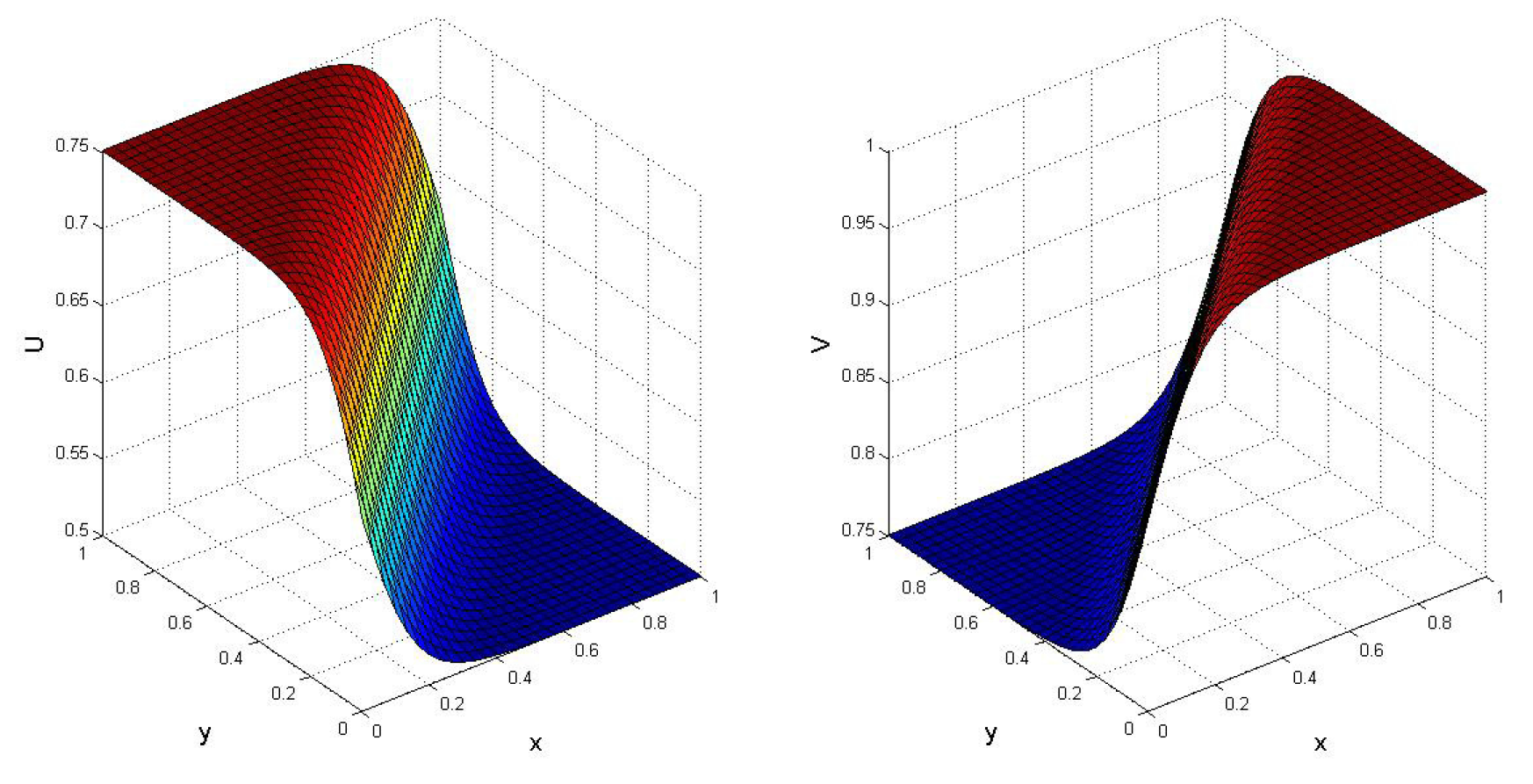
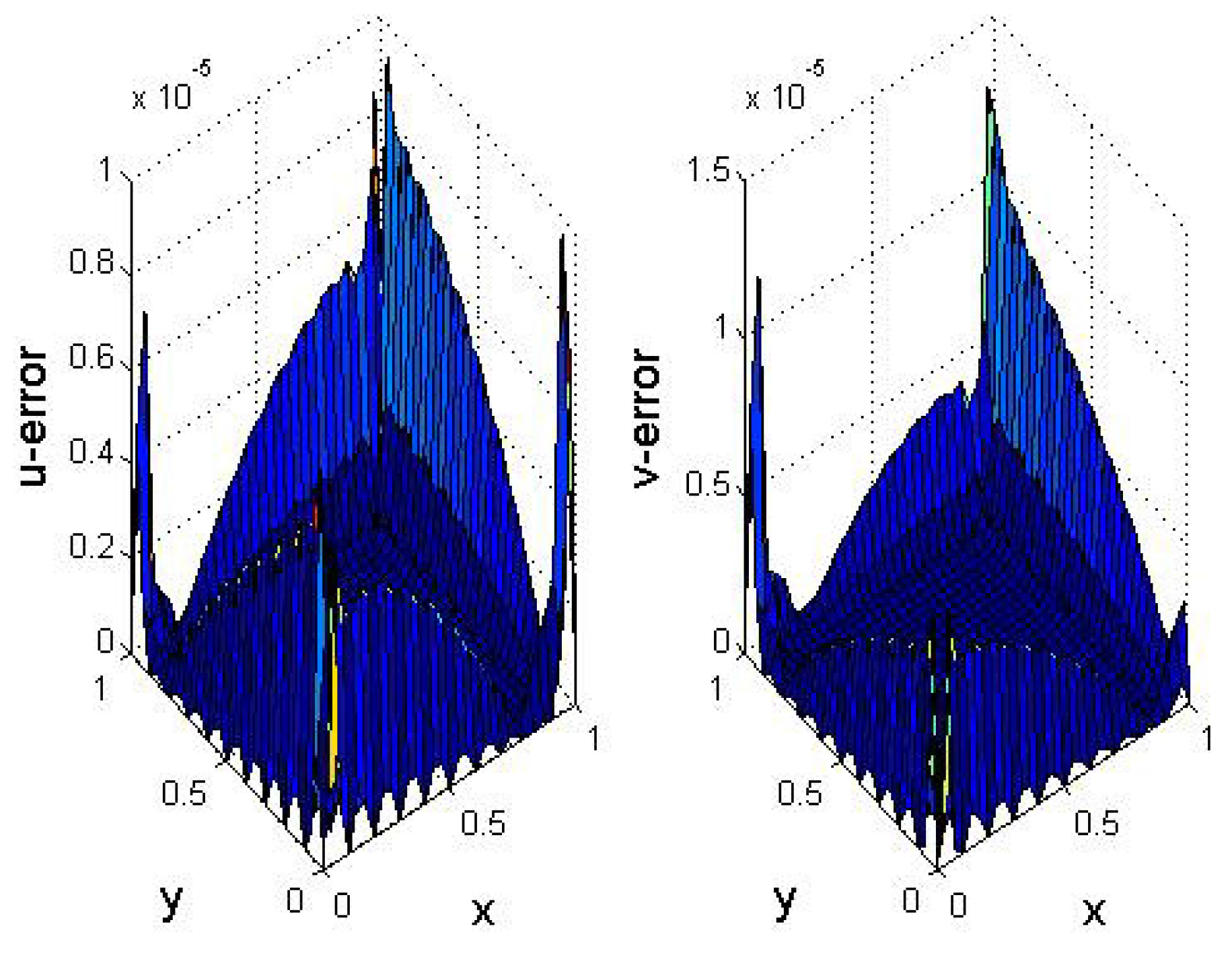
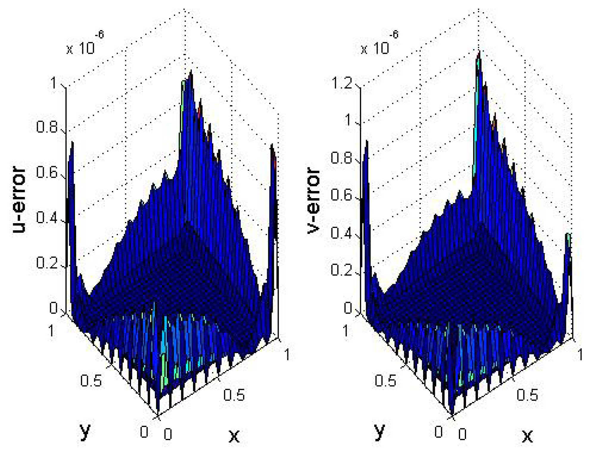
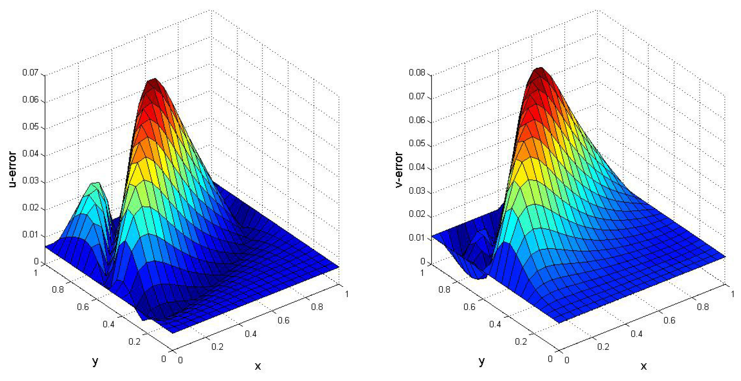
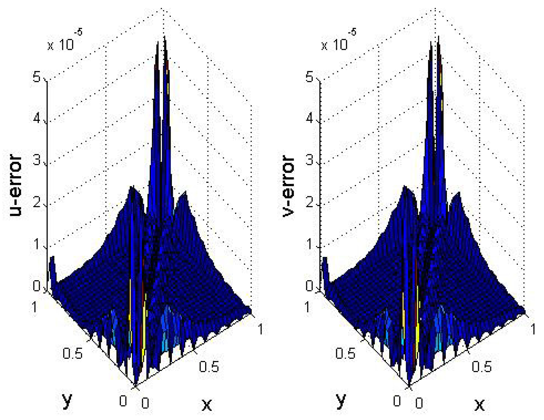
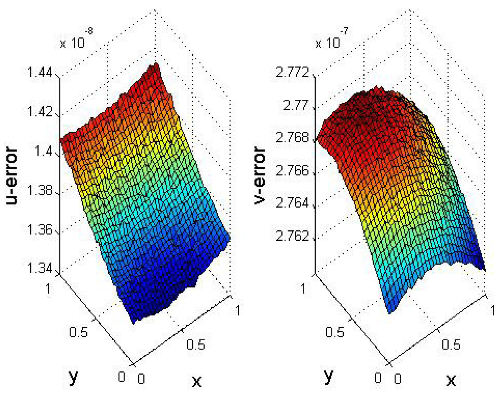
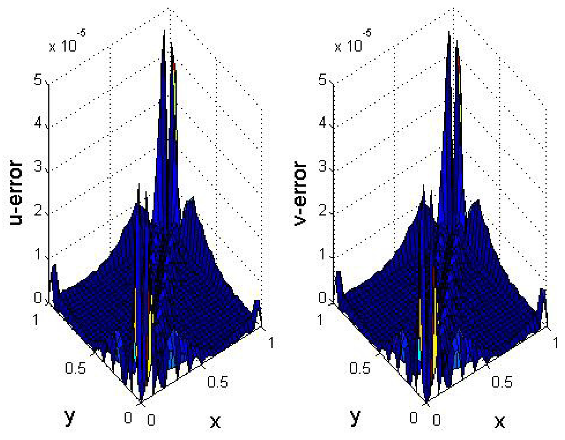
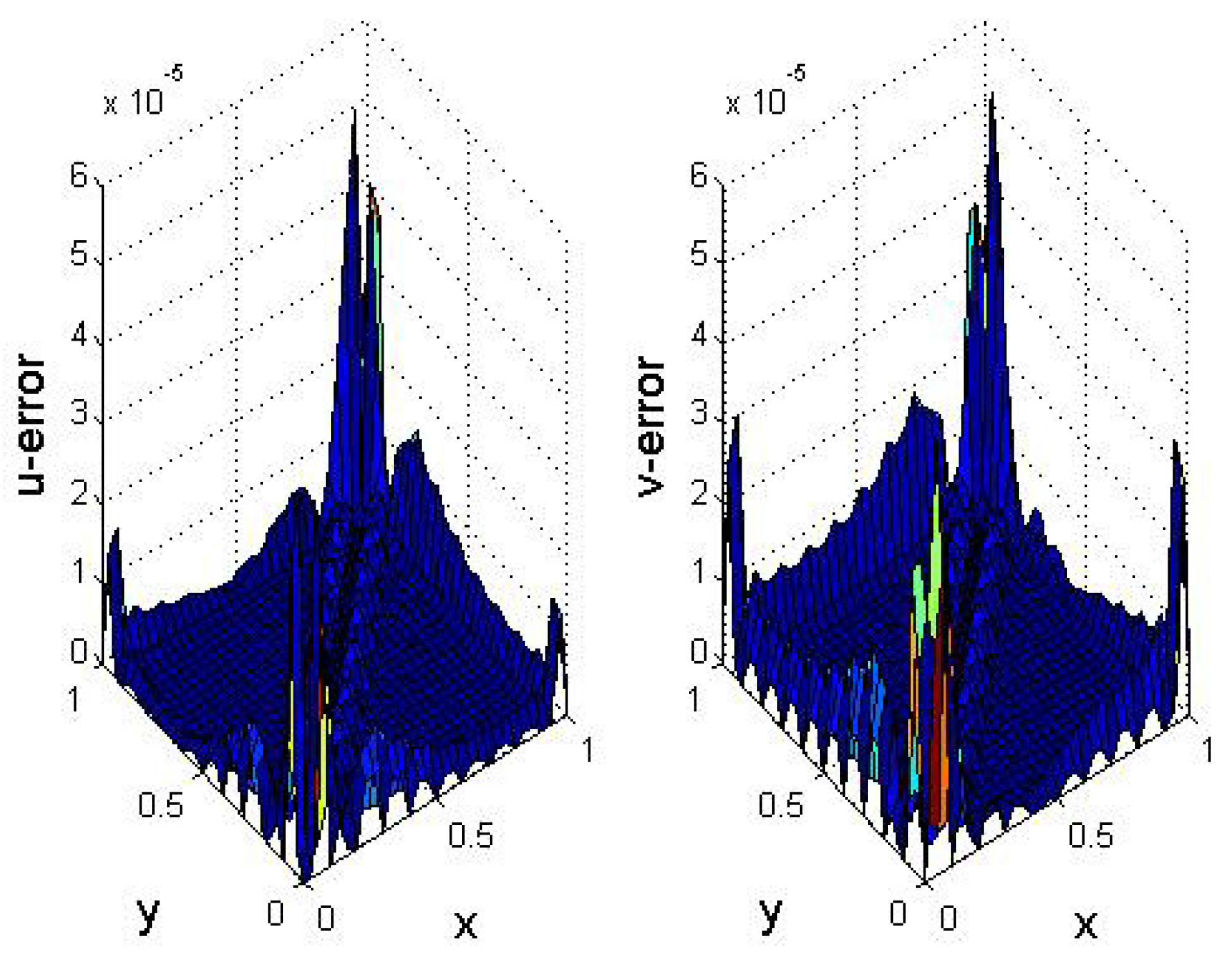
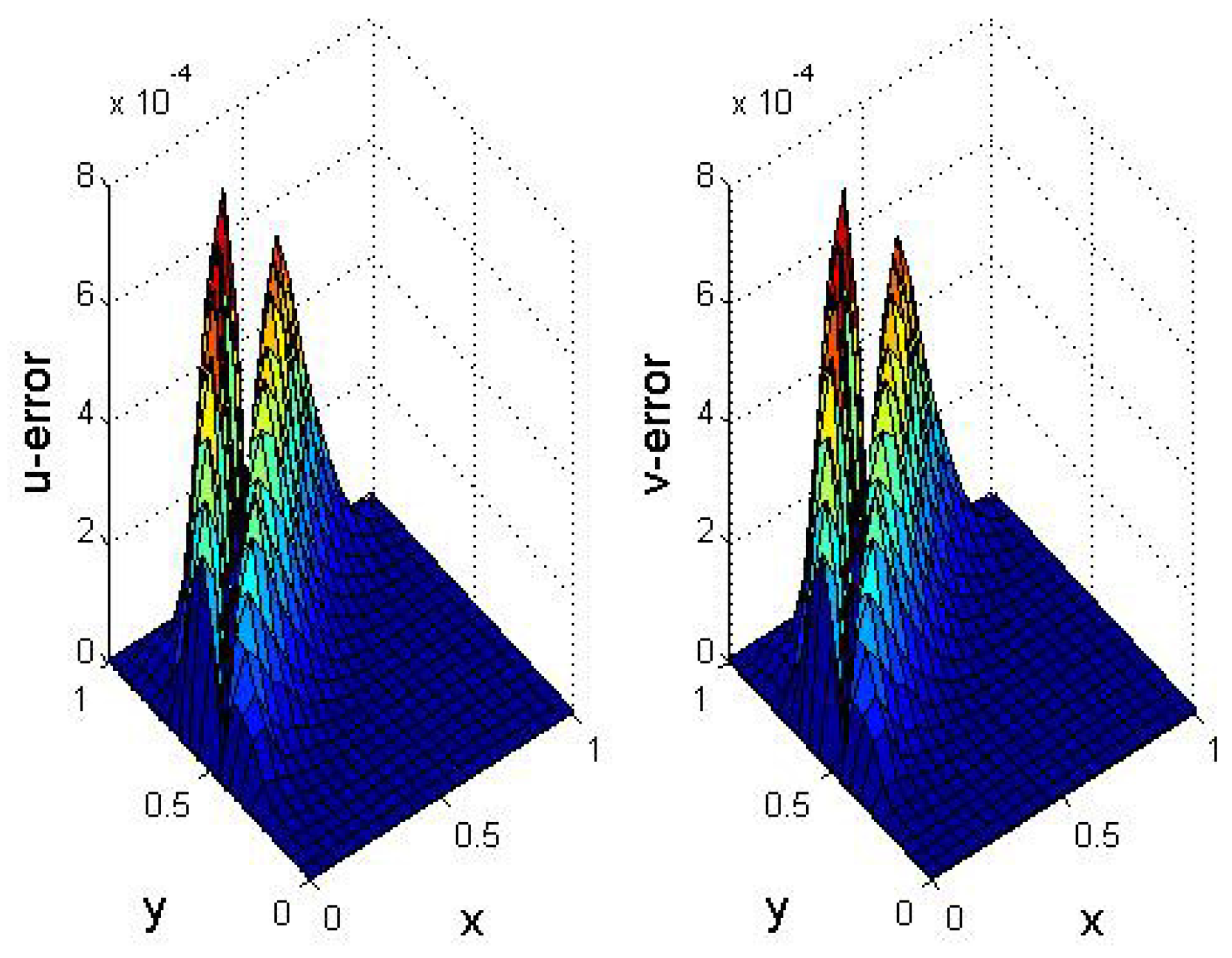
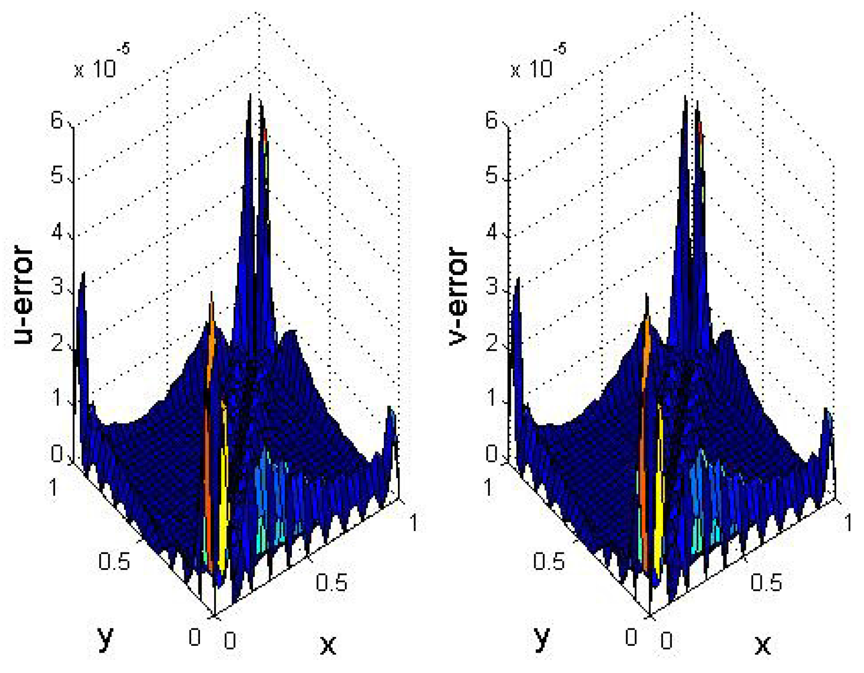
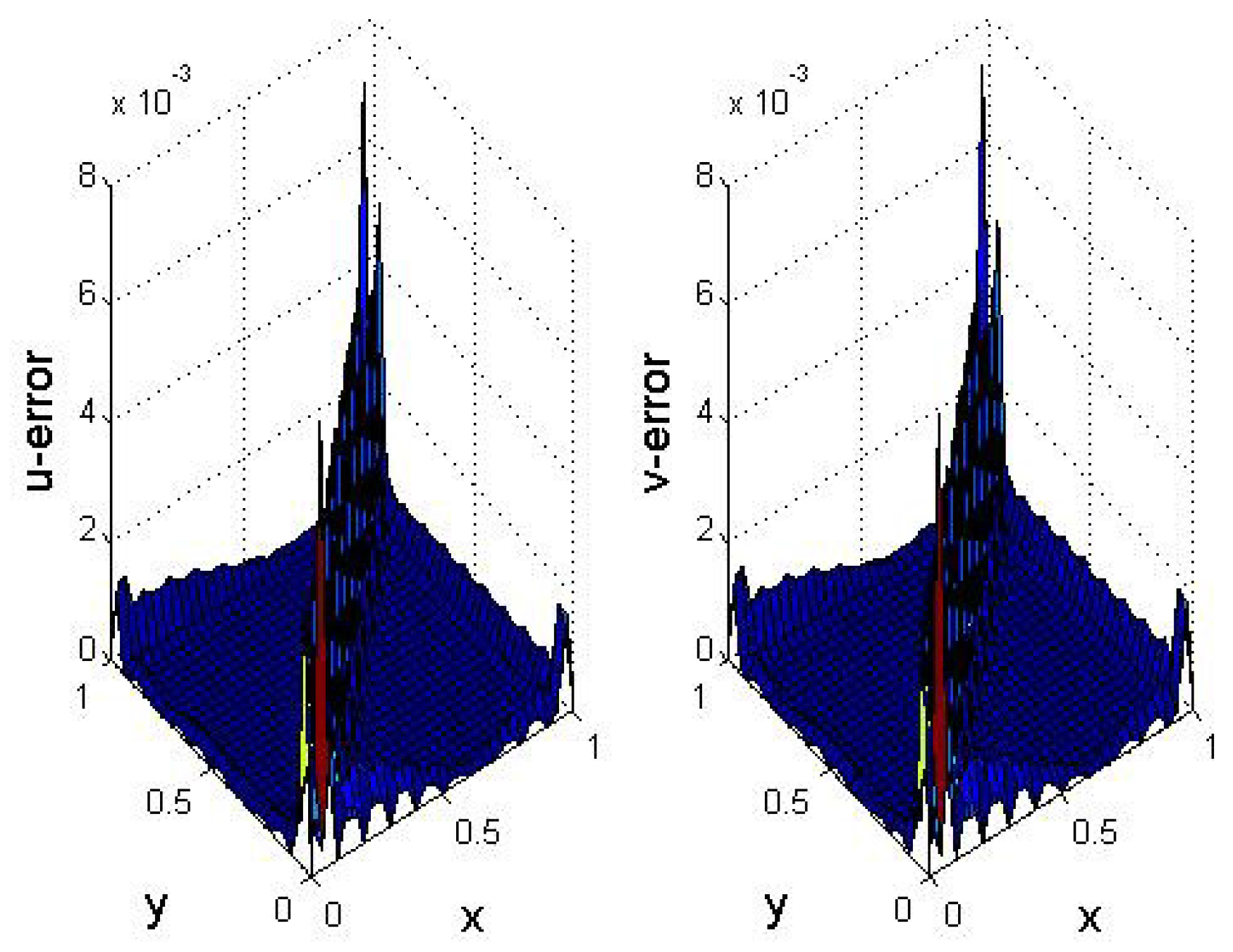
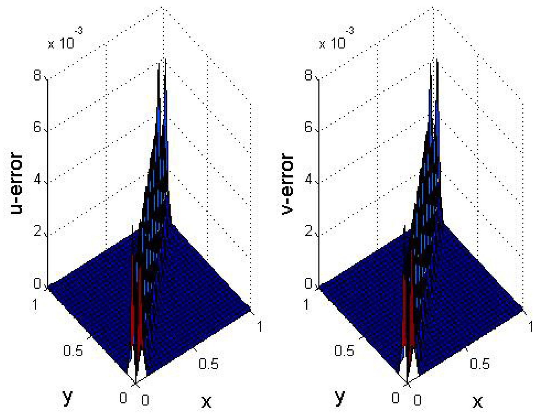
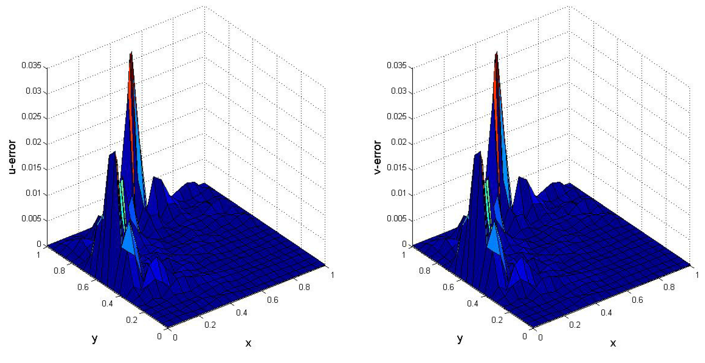
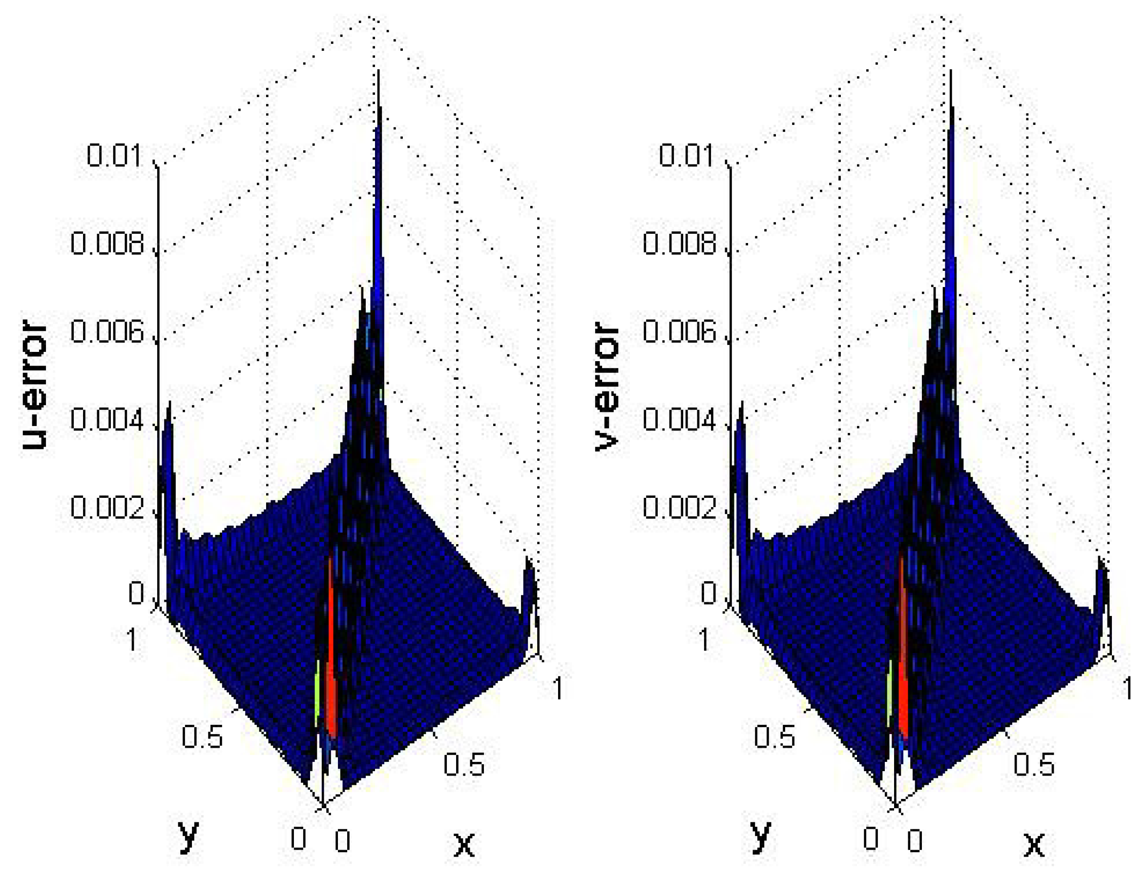
Large values of Re lead to sharp gradients in the solutions as shown in Figure 2. The solutions of singularly perturbed problems exhibit sharp boundary or/and interior layers, where the solutions have a steep gradient. Analytical and numerical aspects of singularly perturbed problems are considered by Das et al. [44]. Figure 3 and Figure 4 show absolute error distributions at time T = 2 for R e = 10 with strategy 3 for different number of points. These figures show, if we increase nodes, absolute error decreases. The absolute error distributions at time T = 2 for R e =100 with CSP are shown in Figure 5, Figure 6 and Figure 7 with a different number of points showing the absolute error distributions at time T = 2 for R e =100. It can be seen that the error decreases with an increasing the number of points. Figure 8, Figure 9, Figure 10, Figure 11 and Figure 12 present absolute error distributions at time T = 2 for R e =100 with different shape strategies. Figure 13 presents absolute error distributions at time T = 2 for R e =1000 by CSP. Figure 14, Figure 15, Figure 16 and Figure 17 show absolute error distributions at time T = 2 for R e =1000 with different shape strategies.
In Table 1 and Table 2, performance of the method is compared with the other methods [24,27,31,35] at selected points. It can be noted that the numerical results obtained from the proposed method are fairly accurate.
Example 2.
Consider problems (14)–(16) with the following initial and mixed boundary conditions given by [32]:
U ( x , y , 0 ) = sin ( π x ) cos ( π y ) , V ( x , y , 0 ) = cos ( π x ) sin ( π y ) , U ( o , y , t ) = U ( 1 , y , t ) = 0 , V ( x , 0 , t ) = V ( x , 1 , t ) = 0 , U n ( x , 0 , t ) = U n ( x , 1 , t ) = 0 , V n ( 0 , y , t ) = V n ( 1 , y , t ) = 0 .
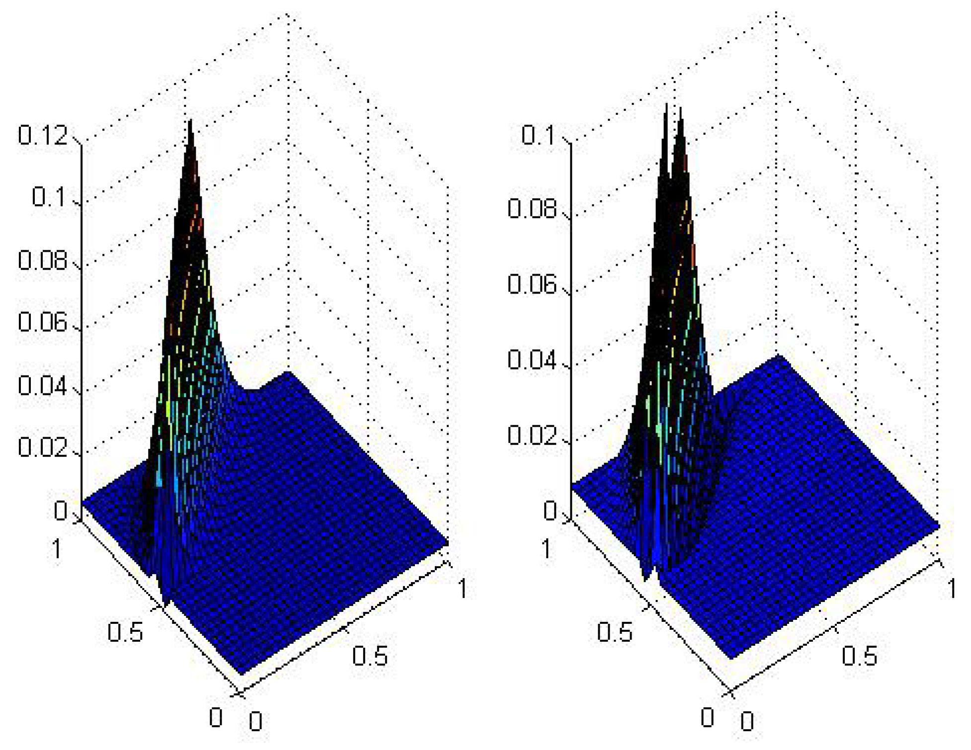
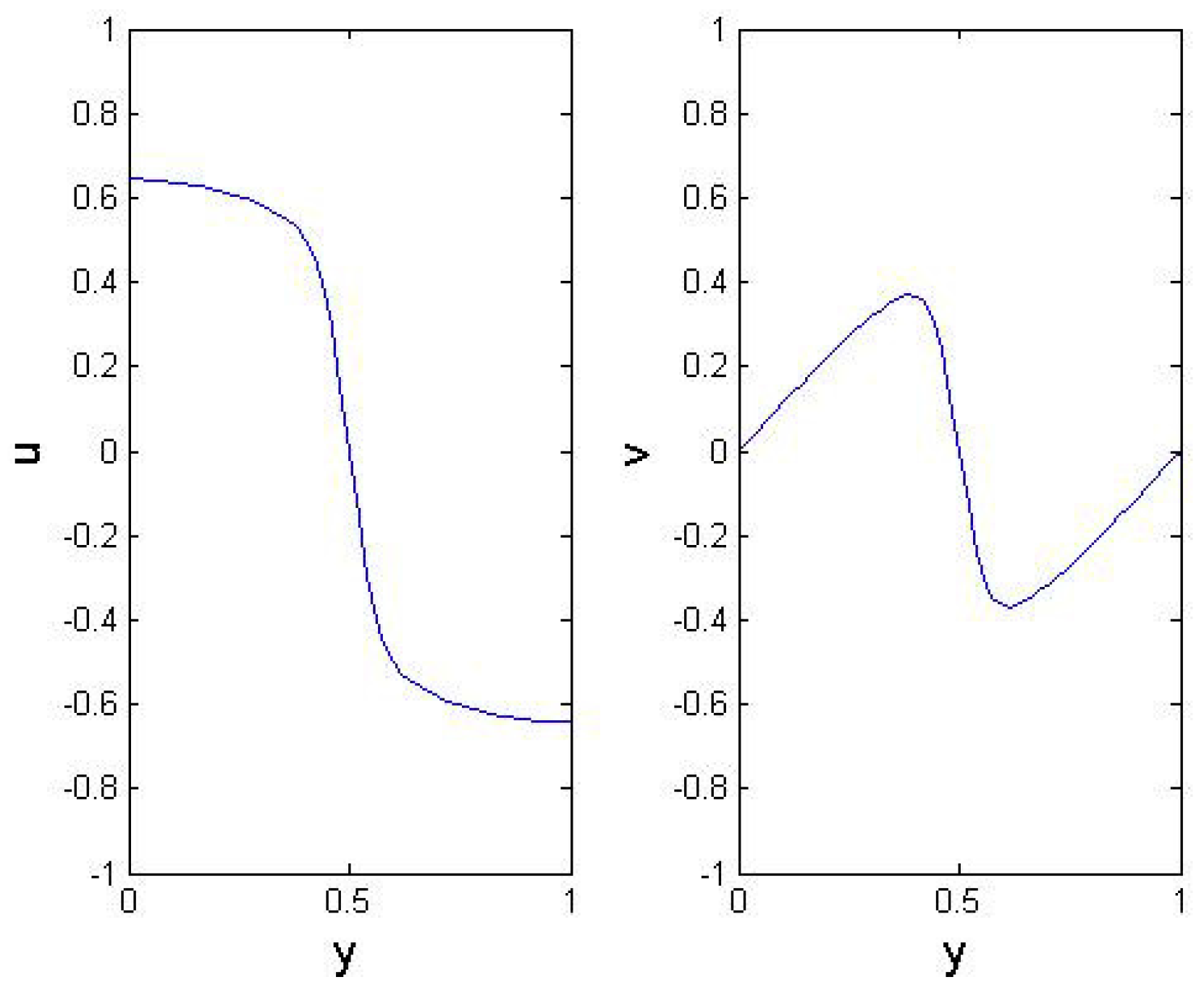
We will compare the obtained solution in our proposed method with the results described in [11,35] because there is not the exact solution. Fake oscillations have been observed by using finite element method (FEM), finite-difference method (FDM), element free Galerkin method [32] and Galerkin-reproducing kernel method [11]. In [35], an adaptive upwind technique has been innovated to avoid wiggles in the recommended local RBF collocation method. As mentioned in [11], even a very fine grid cannot get rid of the oscillatory behavior caused by a sharp gradient. To omit the wiggles and defeat instabilities for R e = 1000 , we have used RBFs with CSP as shown in Figure 18.
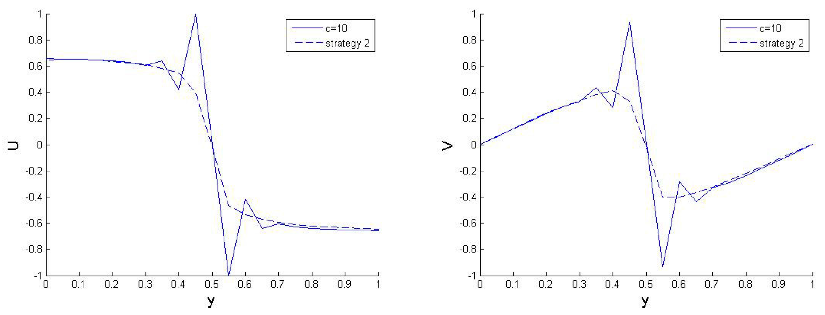
The solution is smooth and near the front we do not have any instability for small R e and, therefore, no VSP is required. In our case, for R e = 10 , 000 , Figure 19 shows the oscillatory behavior. To avoid these wiggles, we have used VSP (strategy 2) in order to stabilize the solution near the sharp front.

6. Conclusions

Six shape parameter strategies were compared in this study. One strategy used a constant shape, while the other five used a different value of the shape parameter at each center. Results show that VSPs can improve the condition number and the solution accuracy. The approach is successfully applied to solve the 2D nonlinear coupled Burgers’ equations with Dirichlet boundary conditions for high Re . Owing to Neumann boundary conditions, instabilities appear near the sharp gradient without any special filtering technique for R e = 1000, 10,000 for mixed boundary conditions. These fake oscillations were also observed using the FDM, FEM and element free Galerkin methods. In [35], an adaptive upwind technique was devised to avoid these wiggles for R e = 1000 . To get rid of the oscillatory behavior, we proposed constant and VSP for R e = 1000, 10,000, respectively.

Acknowledgments

The authors are very grateful to reviewers for carefully reading this paper and for their comments and suggestions which have improved the paper.

Author Contributions

All authors contributed equally and significantly to the study and preparation of the article. They have read and approved the final manuscript.

Conflicts of Interest

The authors declare no conflict of interest.

References

  1. Belytschko, T.; Krongauz, Y.; Organ, D.; Fleming, M.; Krysl, P. Meshless methods: An overview and recent developments. Comput. Methods Appl. Mech. Eng. 1996, 139, 3–47. [Google Scholar] [CrossRef]
  2. Franke, C.; Schaback, R. Convergence order estimates of meshless collocation methods using radial basis functions. Adv. Comput. Math. 1998, 8, 381–399. [Google Scholar] [CrossRef]
  3. Franke, C.; Schaback, R. Solving partial differential equations by collocation using radial basis functions. Appl. Math. Comput. 1998, 93, 73–82. [Google Scholar] [CrossRef]
  4. Kansa, E.J. Application of Hardy’s multiquadric interpolation to hydrodynamics. In Proceedings of the Society for Computer Simulation (SCS) Multiconference, San Diego, CA, USA, 23–25 January 1986; Volume 4, pp. 111–117. [Google Scholar]
  5. Schaback, R. A computational tool for comparing all linear PDE solvers. Adv. Comp. Math. 2015, 41, 333–355. [Google Scholar] [CrossRef]
  6. Schaback, R.; Wendland, H. Kernel techniques: From machine learning to meshless methods. Acta Numer. 2006, 15, 543–639. [Google Scholar] [CrossRef]
  7. Abbasbandy, S.; Azarnavid, B.; Alhuthali, M.S. A shooting reproducing kernel Hilbert space method for multiple solutions of nonlinear boundary value problems. J. Comput. Appl. Math. 2015, 279, 293–305. [Google Scholar] [CrossRef]
  8. Azarnavid, B.; Parvaneh, F.; Abbasbandy, S. Picard-Reproducing kernel Hilbert space method for solving generalized singular nonlinear Lane-Emden type equations. Math. Model. Anal. 2015, 20, 754–767. [Google Scholar] [CrossRef]
  9. Hon, Y.; Schaback, R. Solvability of partial differential equations by meshless kernel methods. Adv. Comput. Math. 2008, 28, 283–299. [Google Scholar] [CrossRef]
  10. Lee, C.F.; Ling, L.; Schaback, R. On convergent numerical algorithms for unsymmetric collocation. Adv. Comput. Math. 2009, 30, 339–354. [Google Scholar] [CrossRef]
  11. Mohammadi, M.; Mokhtari, R.; Panahipour, H. A Galerkin-reproducing kernel method: Application to the 2D nonlinear coupled Burgers’ equations. Eng. Anal. Bound. Elem. 2013, 37, 1642–1652. [Google Scholar] [CrossRef]
  12. Mohammadi, M.; Mokhtari, R.; Schaback, R. A meshless method for solving the 2D Brusselator reaction-diffusion system. Comput. Model. Eng. Sci. 2014, 101, 113–138. [Google Scholar]
  13. Bozzini, M.; Lenarduzzi, L.; Rossini, M.; Schaback, R. Interpolation with variably scaled kernels. IMA J. Numer. Anal. 2015, 35, 199–219. [Google Scholar] [CrossRef]
  14. Hardy, R.L. Multiquadric equations of topography and other irregular surfaces. J. Geophys. Res. 1971, 76, 1905–1915. [Google Scholar] [CrossRef]
  15. Huang, C.S.; Lee, C.F.; Cheng, A.D. Error estimate, optimal shape factor, and high precision computation of multiquadric collocation method. Eng. Anal. Bound. Elem. 2007, 31, 614–623. [Google Scholar] [CrossRef]
  16. Kansa, E.J.; Aldredge, R.C.; Ling, L. Numerical simulation of two-dimensional combustion using mesh-free methods. Eng. Anal. Bound. Elem. 2009, 33, 940–950. [Google Scholar] [CrossRef]
  17. Sarra, S.A.; Sturgill, D. A random variable shape parameter strategy for radial basis function approximation methods. Eng. Anal. Bound. Elem. 2009, 33, 1239–1245. [Google Scholar] [CrossRef]
  18. Golbabai, A.; Rabiei, H. Hybrid shape parameter strategy for the RBF approximation of vibrating systems. Int. J. Comput. Math. 2012, 89, 2410–2427. [Google Scholar] [CrossRef]
  19. Dehghan, M.; Mohammadi, V. The method of variably scaled radial kernels for solving two-dimensional magnetohydrodynamic (MHD) equations using two discretizations: The Crank-Nicolson scheme and the method of lines (MOL). Comput. Math. Appl. 2015, 70, 2292–2315. [Google Scholar] [CrossRef]
  20. Dereli, Y.; Schaback, R. The meshless kernel-based method of lines for solving the equal width equation. Appl. Math. Comp. 2013, 219, 5224–5232. [Google Scholar] [CrossRef]
  21. Mavrič, B.; Šarler, B. Local radial basis function collocation method for linear thermoelasticity in two dimensions. Int. J. Numer. Methods Heart Fluid Flow 2015, 25, 1488–1510. [Google Scholar] [CrossRef]
  22. Sarra, S. A local radial basis function method for advection-diffusion-reaction equations on complexly shaped domains. Appl. Math. Comp. 2012, 218, 9853–9865. [Google Scholar] [CrossRef]
  23. Burger, J.M. A mathematical model illustrating the theory of turbulence. Adv. Appl. Mech. 1948, 1, 171–199. [Google Scholar]
  24. Ali, A.; Islam, S.U.; Haq, S. A computational meshfree technique for the numerical solution of the two-dimensional coupled Burgers’ equations. Int. J. Comput. Methods Eng. Sci. Mech. 2009, 10, 406–412. [Google Scholar] [CrossRef]
  25. Nee, J.; Duan, J. Limit set of trajectories of the coupled viscous Burgers’ equations. Appl. Math. Lett. 1998, 11, 57–61. [Google Scholar] [CrossRef]
  26. Perko, J.; Šarler, B. Weight function shape parameter optimization in meshless methods for non-uniform grids. Comput. Model. Eng. Sci. 2007, 19, 55–68. [Google Scholar]
  27. Younga, D.; Fana, C.; Hua, S.; Alturi, S. The Eulerian-Lagrangian method of fundamental solutions for two-dimensional unsteady Burgers’ equations. Eng. Anal. Bound. Elem. 2009, 32, 395–412. [Google Scholar] [CrossRef]
  28. Fletcher, J.D. Generating exact solutions of the two-dimensional Burgers’ equations. Int. J. Numer. Methods Fluids 1983, 3, 213–216. [Google Scholar] [CrossRef]
  29. Mokhtari, R.; Mohammadi, M. New exact solutions to a class of coupled nonlinear PDEs. Int. J. Nonlinear Sci. Numer. Simul. 2009, 10, 779–796. [Google Scholar] [CrossRef]
  30. Fletcher, C.A.J. A comparison of finite element and finite difference solution of the one and two dimensional Burgers’ equations. J. Comput. Phys. 1983, 51, 159–188. [Google Scholar] [CrossRef]
  31. Bahdir, A.R. A fully implicit finite difference scheme for two dimensional Burgers’ equations. Appl. Math. Comput. 2003, 137, 131–137. [Google Scholar]
  32. Zhang, X.H.; Ouyang, J.; Zhang, L. Element-free characteristic Galerkin method for Burgers’ equation. Eng. Anal. Bound. Elem. 2009, 33, 356–362. [Google Scholar] [CrossRef]
  33. Zhang, L.; Ouyang, J.; Wang, X.; Zhang, X. Variational multiscale element-free Galerkin method for 2D Burgers’ equation. J. Comput. Phys. 2010, 29, 7147–7161. [Google Scholar] [CrossRef]
  34. Zhang, W.; Ahang, C.; Xi, G. An explicit Chebyshev pseudospectral multigrid method for incompressible Navier-Stokes equations. Comput. Fluids 2010, 39, 178–188. [Google Scholar] [CrossRef]
  35. Šarler, B.; Vertnik, R.; Kosec, G. Radial basis function collocation method for the numerical solution of the two-dimensional transient nonlinear coupled Burgers’ equations. Appl. Math. Model. 2012, 36, 1148–1160. [Google Scholar]
  36. Wendland, H. Scattered data approximation. In Cambridge Mongraph on Applied and Computational Mathematics; Cambridge University Press: Cambridge, UK, 2005. [Google Scholar]
  37. Buhmann, M.D. Radial Basis Functions; Cambridge University Press: Cambridge, UK, 2004. [Google Scholar]
  38. Schaback, R. Kernel–Based Meshless Methods. Available online: http://num.math.uni-goettingen.de/schaback/teaching/Appverf-II.pdf (access on 18 July 2007).
  39. Sanyasiraju, Y.; Satyanarayana, C. On optimization of the RBF shape parameter in a grid-free local scheme for convection dominated problems over non-uniform centers. Appl. Math. Model. 2013, 37, 7245–7272. [Google Scholar] [CrossRef]
  40. Dehghan, M.; Mohammadi, V. The numerical solution of Fokker–Planck equation with radial basis functions (RBFs) based on the meshless technique of Kansa’s approach and Galerkin method. Eng. Anal. Bound. Elem. 2014, 47, 38–63. [Google Scholar] [CrossRef]
  41. Kansa, E.J. Multiquadrics—A scattered data approximation scheme with applications to computational fluid dynamics I: Surface approximations and partial derivative estimates. Comput. Math. Appl. 1990, 19, 127–145. [Google Scholar] [CrossRef]
  42. Kansa, E.J. Multiquadrics—A scattered data approximation scheme with applications to computational fluid dynamics II: Solutions to parabolic hyperbolic, and elliptic partial differential equations. Comput. Math. Appl. 1990, 19, 147–161. [Google Scholar] [CrossRef]
  43. Xiang, S.; Wang, K.M.; Ai, Y.T.; Sha, Y.D.; Shi, H. Trigonometric variable shape parameter and exponent strategy for generalized multiquadric radial basis function approximation. Appl. Math. Model. 2012, 36, 1931–1938. [Google Scholar] [CrossRef]
  44. Das, P.; Natesan, S. Adaptive mesh generation for singularly perturbed fourth-order ordinary differential equations. J. Comput. Math. 2015, 92, 562–578. [Google Scholar] [CrossRef]
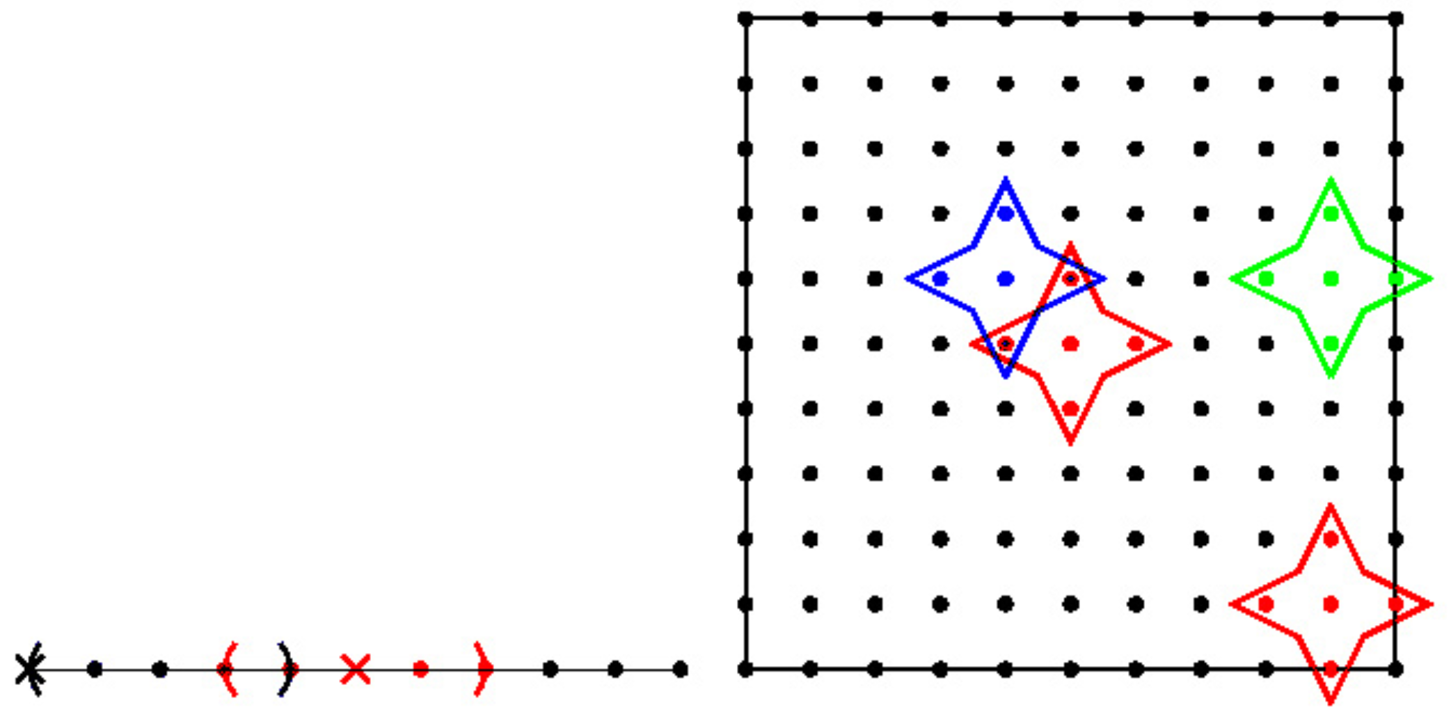
Figure 1. The uniform node arrangement and the schematics of the local domains of influence in the interior, near boundary and corner points using n s = 5 , 1D (left), and 2D (right), where × denotes the center node in 1D.
Mathematics 05 00038 g001
Figure 2. Numerical solution of U and V at time T = 2 with R e = 100 , n = 1681 , strategy 1 (Test problem 1).
Mathematics 05 00038 g002
Figure 3. Absolute error graphs at time T = 2 with R e = 10 , n = 441 , strategy 3 (test problem 1).
Mathematics 05 00038 g003
Figure 4. Absolute error graphs at time T = 2 with R e = 10 , n = 1681 , strategy 3 (test problem 1).
Mathematics 05 00038 g004
Figure 5. Absolute error graphs at time T = 2 with R e = 100 , n = 1681 , c = 10 (test problem 1).
Mathematics 05 00038 g005
Figure 6. Absolute error graphs at time T = 2 with R e = 100 , n = 1681 , strategy 1 (test problem 1).
Mathematics 05 00038 g006
Figure 7. Absolute error graphs at time T = 2 with R e = 100 , n = 3721 , strategy 1 (test problem 1).
Mathematics 05 00038 g007
Figure 8. Absolute error graphs at time T = 2 with R e = 100 , n = 1681 , strategy 2 (test problem 1).
Mathematics 05 00038 g008
Figure 9. Absolute error graphs at time T = 2 with R e = 100 , n = 1681 , strategy 3 (test problem 1).
Mathematics 05 00038 g009
Figure 10. Absolute error graphs at time T = 2 with R e = 100 , n = 1681 , strategy 4 (test problem 1).
Mathematics 05 00038 g010
Figure 11. Absolute error graphs at time T = 2 with R e = 100 , n = 1681 , strategy 4 (legender points) (test problem 1).
Mathematics 05 00038 g011
Figure 12. Absolute error graphs at time T = 2 with R e = 100 , n = 1681 , strategy 5 (test problem 1).
Mathematics 05 00038 g012
Figure 13. Absolute error graphs at time T = 2 with R e = 1000 , n = 1681 , c = 10 (test problem 1).
Mathematics 05 00038 g013
Figure 14. Absolute error graphs at time T = 2 with R e = 1000 , n = 1681 , strategy 2 (test problem 1).
Mathematics 05 00038 g014
Figure 15. Absolute error graphs at time T = 2 with R e = 1000 , n = 1681 , strategy 3 (test problem 1).
Mathematics 05 00038 g015
Figure 16. Absolute error graphs at time T = 2 with R e = 1000 , n = 1681 , strategy 4 (test problem 1).
Mathematics 05 00038 g016
Figure 17. Absolute error graphs at time T = 2 with R e = 1000 , n = 1681 , strategy 5 (test problem 1).
Mathematics 05 00038 g017
Figure 18. Numerical results at time T = 0.4 , x = 0.5 , with R e = 1000 , c = 10 , n = 441 , on the left U and on the right V. (test problem 2)
Mathematics 05 00038 g018
Figure 19. Numerical results at time T = 0.4 , x = 0.5 , with R e = 10000 , n = 441 Legendre points, on the left U and on the right V. (test problem 2)
Mathematics 05 00038 g019
Table 1. Numerical results for U at time T = 2 with R e = 100 , n = 441 .
( x , y ) ( 0.1 , 0.1 ) ( 0.3 , 0.3 ) ( 0.5 , 0.5 ) ( 0.3 , 0.7 ) ( 0.1 , 0.9 ) ( 0.5 , 0.9 )
Exact 0.500482 0.500482 0.500482 0.555675 0.744256 0.555675
Strategy 4 0.500490 0.500514 0.500528 0.554754 0.744165 0.555365
[35] 0.500470 0.500441 0.500414 0.554805 0.744197 0.554489
[24] 0.50035 0.50042 0.50046 0.55609 0.74409 0.55604
[31] 0.49983 0.49977 0.49973 0.55429 0.74340 0.55413
[27] 0.50012 0.50042 0.50041 0.55413 0.74416 0.55637
Table 2. Numerical results for V at time T = 2 with R e = 100 , n = 441 .
( x , y ) ( 0.1 , 0.1 ) ( 0.3 , 0.3 ) ( 0.5 , 0.5 ) ( 0.3 , 0.7 ) ( 0.1 , 0.9 ) ( 0.5 , 0.9 )
Exact 0.999518 0.999518 0.999518 0.944325 0.755744 0.944325
Strategy 4 0.999537 0.999582 0.999617 0.945206 0.755867 0.944679
[35] 0.999530 0.999559 0.999586 0.945195 0.755803 0.945511
[24] 0.99936 0.99951 0.99958 0.94387 0.75592 0.94392
[31] 0.99826 0.99861 0.99821 0.94409 0.75500 0.94441
[27] 0.99946 0.99938 0.99941 0.94387 0.75558 0.94345