An Optimal Control Approach for the Treatment of Solid Tumors with Angiogenesis Inhibitors


1
Department of Nuclear Engineering, University of California, Berkeley, Berkeley, CA 94720, USA
2
School of Science, Penn State Erie, The Behrend College, Erie, PA 16563, USA
*
Author to whom correspondence should be addressed.
†
These authors contributed equally to this work.
Mathematics 2017, 5(4), 49; https://doi.org/10.3390/math5040049
Submission received: 24 June 2017
/
Revised: 14 September 2017
/
Accepted: 29 September 2017
/
Published: 10 October 2017
Abstract
:Cancer is a disease of unregulated cell growth that is estimated to kill over 600,000 people in the United States in 2017 according to the National Institute of Health. While there are several therapies to treat cancer, tumor resistance to these therapies is a concern. Drug therapies have been developed that attack proliferating endothelial cells instead of the tumor in an attempt to create a therapy that is resistant to resistance in contrast to other forms of treatment such as chemotherapy and radiation therapy. In this study, a two-compartment model in terms of differential equations is presented in order to determine the optimal protocol for the delivery of anti-angiogenesis therapy. Optimal control theory is applied to the model with a range of anti-angiogenesis doses to determine optimal doses to minimize tumor volume at the end of a two week treatment and minimize drug toxicity to the patient. Applying a continuous optimal control protocol to our model of angiogenesis and tumor cell growth shows promising results for tumor control while minimizing the toxicity to the patients. By investigating a variety of doses, we determine that the optimal angiogenesis inhibitor dose is in the range of 10–20 mg/kg. In this clinically useful range of doses, good tumor control is achieved for a two week treatment period. This work shows that varying the toxicity of the treatment to the patient will change the optimal dosing scheme but tumor control can still be achieved.
1. Background
Cancer is a disease of unregulated cell growth. Unlike normal adult cells that divide only to replace dead or dying cells, cancer cells continue to grow, forming more abnormal cells. Typically cancerous cells arise when proto-oncogenes undergo a genetic change and become oncogenes, or tumorcoding genes. Cancer cells are often found to contain broken or morphed chromosomes that can cause irregular gene expression. Cancer invades healthy cells to obtain nutrients by parasitising its host organism. According to the National Institute of Health’s National Cancer Institute, 1.6 million new cases of cancer are predicted to be diagnosed in 2017 and over 600,000 people would die from the disease [1,2].
Chemotherapy is a common treatment for cancer control. The chemotherapy process adds drugs into a person’s body to kill cancerous cells, prevent the cells from dividing, and prevent the spread of cancer into other parts of the body. The majority of chemotherapy agents do not target cancer cells selectively so they also harm healthy cells. Part of this is due to the drugs dispersal throughout the body and not centralized in the spot of the cancerous cells. The goal of chemotherapy is to kill the cancerous cells with minimal damage to healthy tissue. Chemotherapy agents’ lack of selectivity means that time is a factor when administering therapy. Time will help determine how much damage is done to healthy tissues. While there are many treatments out there for fighting cancer, there is no real cure for this disease. Although chemotherapy is an effective tool in the fight against cancer, the side effects of the compounds are a limiting factor for how much dose can be applied. The rapid cellular division of cancer also means that it can easily become resistant to the chemotherapeutic agents used to fight this disease. This has been argued to be the leading cause of cancer mortality [3,4]. If treatment resistance can be overcome, then cancer mortality would decrease. This implication has provided the impetus for further study into either reducing chemotherapy resistance or finding alternative therapies that would be immune to resistance [5].
Chemotherapy is often coupled with radiation therapy and surgery to improve survival of patients with solid tumors. Fine et al. [6] showed that coupling chemotherapy with post-operative radiation therapy has advantageous effects on patients with malignant gliomas. Li et al. [7] verified Fine’s results with a three cohort study that showed coupling radiation and chemotherapy greatly reduces the risk of metastases. Fine concluded that hypoxic tumors are generally resistant to radiation therapy. The goal of radiation therapy is to create free radical oxygen agents that will enter the cell nucleus and destroy DNA molecules, effectively killing the tumor cells. Therfore hypoxic tumors are often termed radioresistant since free radicals cannot be created. These conclusions have been studied extensively and now models are coming out to assess the extent of radioresistance a tumor has based on its level of hypoxia [8]. Despite being an effective treatment to gain local control of solid tumors, radiation therapy often has side effects, including radiation burns, and short and long term damage to normal tissues and organs [9].
One alternative to both chemotherapy and radiation therapy is termed anti-angiogenesis therapy. This therapy can be used as a preoperative therapy or in combination with radiation and chemotherapy. There is currently debate whether or not anti-angiogenesis therapy alone can cure a patient of their tumor or if a combination of therapies is required to achieve this cure [10].
Angiogenesis is the proliferation of endothelial cells from healthy human tissue to an organ. Endothelial cells carry blood, nutrients, and oxygen to vital organs and carry de-oxygenated blood away from these organs. While this process is vital in the embryonic stage of development for human life, it is also a means by which tumors survive, grow, and spread. Vascular endothelial growth factor (VEGF) plays the primary role in the development and migration of these tissues [11]. Solid tumors use this phenomenon to attract blood vessels from normal tissues in order to acquire a supply of necessary nutrients and oxygen for growth. Solid tumors must attract blood vessels from their host as they cannot proliferate beyond 1–2 mm without this supply of oxygen and nutrients [12]. The four stages of angiogenesis are initiation, promotion, progression, and metastasis that are described below.
A tumor will send out chemicals during the initiation stage, such as VEGF, to promote endothelial cells to begin proliferation. The nearby endothelial cells are catalyzed by the VEGF molecules and begin to promote outwards towards the tumor. The endothelial cells reach the tumor in the progression stage and are able to supply it with necessary nutrients, such as glucose and oxygen. Metastasis can then occur when cells from the initial lesion break off and travel through the newly proliferated endothelial cells to anywhere in the body. Certain cancers tend to metastasize to different locations in the body, but in general a patient with metastatic cancer has a higher mortality rate than one with a non-metastatic tumor for a variety of reasons. It is believed that a metastatic tumor can grow a new tumor from just one cell that attaches itself to the host [13]. Multiple tumors accelerate the rate of death of the patient through increased parasitism of nutrients. They also become increasingly harder to treat without greatly increasing the side effects of treatment.
Anti-angiogenesis therapy is a means of preventing the proliferation of endothelial cells so that tumors will not metastasize. So far there are a variety of drugs that have been approved by the FDA which work to prevent angiogenesis, such as Bevacizumab for glioblastoma and Sorafenib for kidney cancer [14]. Unlike other methods of cancer treatment, such as radiation and chemotherapy that target the cancer cells directly, anti-angiogenesis therapy targets normal endothelial cells that migrate to the tumor. Because normal cells do not divide rapidly mutations that could cause resistance are far less common. This treatment has therefore been described as being resistant to resistance. Since anti-angiogenesis therapy targets developing endothelial cells, it is an exceptionally good therapy at treating widely metastatic tumors that have many metastases throughout the body without additional toxicity to the patient [15]. Zetter [15] also concluded that anti-angiogenesis therapy may be most effective when delivered at low doses for long periods of time to prevent dormant micro-metastases from ever becoming active.
Anti-angiogenesis therapy does carry lower risk to the patient compared to chemotherapy and radiation therapy, but there are potential side effects [16]. Some notable consquences include the drug interfering with surgical wounds healing, CNS syndromes, female reproductive tract damage, and damage to other organs that have a high turnover rate of endothelial cells. However, it is hard to predict which patients will exhibit side effects and most can be reversed by stopping treatment [17]. Cook and Figg [18] also discussed the potential side effects of anti-angiogenesis therapy and claimed that while long term therapy seems promising, there is little clinical data to show what the risk factors are for patients. Jain et al. [19] claims that most side effects experienced by patients are due to anti-VEGF drugs and the most common side effect is hypertension. Elice and Rodeghiero claimed that the most severe side effect was hemorrhaging and showed that in patients with squamous cell carcinoma around nine percent of experienced life threatening pulmonary hemorrhage [16]. However they also discussed that there has been no clear mechanism identified by which an anti-VEGF drug could cause a hemorrhage. A phase two trial of Bevacizumab, an anti-VEGF anti-angiogenesis drug, showed that 14 percent of participants experienced side effects at doses of 10 mg/kg in single doses administered intravenously [20].
A variety of mathematical models have been developed over the last few decades to describe the evolution of tumor growth and endothelial cell migration under various cancer therapies [21]. Although these models can focus on different aspects of the evolution of cancer, the modelling process leads to three distinct approaches: continuum models [22]—typically formulated as either ordinary or partial differential equations, discrete models [23], or hybrid models, a combination of the previous two [24,25].
The mathematical models that are most relevant to this study include the work by Hahnfeldt et al. [26], who developed a simple mathematical model based on the notion that tumour growth is a process that ultimately relies on the development of the vasculature. This model assumed that tumour cells produce two distinct factors, one that exerts a stimulatory effect, and another that exerts an inhibitory effect on the vascular network. Sachs et al. [27] proposed a logistic growth model using the clinical data that tumors decelerate in their growth rate as they get larger. They were also the first to develop a model to illustrate the effects of anti-angiogenesis therapy on the growth of angiogenic endothelial cells. To account for tumor vasculature, they include a variable carrying capacity in the overall dynamics that is a balance between stimulation and inhibition of tumor growth factors.
To determine an optimal protocol for anti-angiogenesis therapy, Ergun et al. [28] applied optimal control theory to a slightly modified version of the mathematical model given in [26]. In particular they implemented a bang-bang control in which a fixed amount of angiogenic inhibitors would be used for the duration of the treatment and assumed that maximizing the anti-angiogenic agent dose was equivalent to minimizing the tumor volume. By using this method, Ergun et al. concluded that, as opposed to traditional theory, the largest dose of angiogenesis inhibitors should be given during the second phase of treatment. This work validated the theory of dose escalation proposed by Norton and Simon [29,30]. D’Onofrio and Gandolfi [31] also considered a modified version of the mathematical model given in [26] in which they determined conditions that guarantee the eradication of the tumor under a protocol of periodic anti-angiogenic therapy.
Ledzewicz and Schättler [32] considered the same mathematical model given in [28] but attempted to characterize all parts of the angiogenesis treatment, not just the first two phases. In this work, the authors concluded that the optimal regimen for delivering treatment followed a “0asa0” pattern, where a and 0 denote trajectories with full and no anti-angiogenic therapy, respectively, and s denotes a segment along an optimal singular control. In other words, the solution to their problem is an optimal singular arc that is a concatenation of bang-bang controls—constant controls that give either a full or no dose of inhibitors—and the optimal singular control which administers the inhibitors using a time-dependent schedule at less than a maximum rate. In similar work Ledzewicz and Schättler [33] highlighted that depending on the initial conditions not all of the pieces of the “0asa0” solution proposed in their earlier work are present. In fact, the authors point out that the most typical and medically most relevant scenarios are optimal protocols that take the simple form “a0” in which case all inhibitors are administered at full dose from the beginning or “as0” in which case the dosage is adjusted in a continuous manner until all inhibitors have been exhausted.
As mentioned previously, there are limitations to how large a tumor can grow. Depending on the site of the lesion, a tumor will only grow to a threshold volume before it metastasizes throughout the patient’s body or the patient dies. Current clinical treatments using angiogenesis inhibitors to prevent either of these from happening favor the results from the bang-bang control where a patient receives an injection of a drug over discrete time periods, generally 1–2 injections per week for several weeks, but our research shows that great tumor control can be achieved using the continuous administration of a drug, or daily injections over the course of treatment. Nilsson [34] used single IV injections of scFv(L19)-tTF, an experimental anti-angiogenesis drug for small tumors or three IV injections for large solid tumors, but in both cases, while the tumor growth was inhibited, the tumor did not disappear completely. On the other hand, d’Onofrio et al. [35] did a thorough analysis of the different ways that anti-angiogenesis treatment can be administered. This work concluded that continuous, low doses of the therapeutic drug would produce a better outcome in the eradication of the solid tumor, verifying the conclusions made in [15]. Because of the unfavorable results with bang-bang control and singular arcs for tumors depending on initial conditions, we investigate the two compartment model investigated in [32] but subject it to a continuous optimal control protocol. In [33] there were problems with a linear control where the model deviates from a singular arc which means that the bang-bang control fails to be optimal. We predict that using a quadratic control and following the conclusion in [35] we will resolve these issues.
2. Methods
This paper considers a mathematical model for tumor anti-angiogenesis that was formulated in [28] and is a modification of a previously developed and biologically validated model in [26]. In particular a non-spatial two-compartment cell population model is formulated for the primary tumor volume and endothelial cell volume, which serves as a de facto carrying capacity for the tumor since the maximum tumor volume sustainable by the vascular network that supplies the tumor with nutrients and largely depends on the volume of endothelial cells.
2.1. Mathematical Model
Let p and e represent the primary tumor volume and endothelial cell volume, respectively. Our model follows the work of [28] and [26] by modeling the tumor growth using a Gompertzian growth function resulting in the equations:
where the first and second terms of Equation (2) represent stimulation and inhibition, respectively. Note that Equation (2) has multiple solutions at which is biologically irrelevant. Therefore the substitution is made which transforms the dynamical system given above into [32]:
where represents the tumor growth parameter, b represents the birth of the endothelial cells, d represents the natural death of the endothelial cells, G is the anti-angiogenic dose administered, and u is the time-dependent dose rate control parameter. The values of these parameters and their units can be found in Table 1.
2.2. Steady State Analysis
A linear stability analysis of the steady state is performed first by setting the dose rate . The dynamical system in consideration now has a single steady state solution given by:
To analyze these fixed points, the Jacobian matrix is evaluated at yielding:
which clearly has two negative eigenvalues. This concludes that is a stable node. Despite this result, the model with constant dose rate fails to incorporate the toxicity of the anti-angiogenesis treatment. This issue is addressed by applying optimal control theory in the next section.
2.3. Optimal Control
The objective in this paper is to find the optimal dosage scheme of the anti-angiogenesis drug that minimizes tumor volume at the end of the treatment and reduces the toxic effect of the angiogenesis inhibitors. An optimal control problem is formulated to achieve this objective, defined as:
where the parameter is a balancing weight. Specifically, this work aims to find an optimal control, , such that:
The control is such that where a is equal to the fraction of the total dose that can be administered, therefore . The admissible control set is defined by:
Note that for this system the control set and the objective functional have the appropriate compactness and convexity assumptions to guarantee the existence of an optimal control and the corresponding states [36]. The necessary conditions that an optimal solution must satisfy are derived from the Pontryagin Maximum Principle [37]. This principle converts Equations (3), (4) and (8) into a problem of minimizing pointwise a Hamiltonian function with respect to the control variable . To this end, the Hamiltonian is constructed to be:
where and are the corresponding adjoint variables for the state variables p and x, respectively. According to the Pontryagin Maximum Principle, the system of adjoint equations is found by taking the appropriate partial derivatives of H with respect to the corresponding state variable. For this system, the adjoint equations become:
with transversality conditions:
The characterization of the optimal control is obtained in a straight-forward manner by solving the optimality condition for which yields:
where the bounds on have been taken into consideration . This analysis is summarized in the next paragraph.
Given an optimal control and corresponding solutions and that minimize over , then there exist continuous functions and that satisfy:
Furthermore, the control variable satisfies:
The state system given by Equations (3)–(4), the adjoint system given by Equations (12)–(13) and the characterization of the control given by Equation (14) form the optimality system that is solved in the next section.
The goal of this work is to minimize the optimality system defined by Equation (8). is the total cost to a patient undergoing anti-angiogenesis treatment. It can be seen that it is the summation of the tumor volume at the end of treatment, T, and the integration of the total dose administered at T multiplied by the toxicity parameter of the treatment. This work has shown that minimizing minimizes both the tumor volume and the amount of drug delivered. This can be seen in Figure 1 and Figure 2.
It is worth noting that the parameter in the integrand of Equation (8) denotes what is referred to as a continuous optimal control. This differs from bang-bang and/or singular control found in [32], which arises when the integrand is linear in u. With a continuous optimal control, it is assumed that the drug is being applied continuously over the entire treatment time and that there is no biological drug clearance from the patient’s system. This assumes continuous concentration of angiogenesis inhibitors in the system and attempts to find the optimal concentration of drug by calculating the minimum dose required to minimize the tumor volume at the end of treatment. The total dose at the end of treatment is computed by .
The parameter k is also investigated to determine its effect on the optimal control problem. It is shown that as the value of k increases, the optimal control parameter u changes shape dramatically. Depending on the initial conditions , T, and k the optimal treatment regimen also changes to minimize the tumor volume. This will determine the value of u throughout the treatment time, T. Since u is a percentage of the dose administered over the course of the treatment time T, these results will determine the optimal dose that is administered throughout the study.
The final parameter in this optimal control problem is the treatment time, T. As studied in [11,38,39,40], the delivery time frame of the anti-angiogenesis inhibitors were two to three weeks. This paper defines the treatment time as two weeks to follow the clinical studies already performed for the benefit of verifying biology with mathematics. As opposed to Ledzewicz et al. [32] where the treatment time was left to be determined in the optimal control problem, this work aims to be more representative of medical practice, allowing an easier transition from current practice to the dosing scheme proposed.
3. Results and Discussion
Three different initial conditions are chosen from [26] to define the initial tumor volume ranging between 100 mm and 300 mm. The initial amount of endothelial cells were taken from [32] and is equal to 8000 mm, yielding mm. These numbers are representative of a typical scenario in which a patient begins anti-angiogenesis therapy. The time frame for this study was taken from Goldman et al. [38], Klement et al. [39], and Holash et al. [11] who all performed analyses of anti-angiogenesis drugs on mice over the course of two to three weeks. Shih [40] investigated the effects of anti-angiogensis therapy on patients with a variety of doses ranging from 0.3 to 10 mg/kg also over a two to three week period. This study was performed using a two-week time period assuming that the minimal treatment time would help minimize toxicity to the patient. The doses to study were determined by calculating the cost function over a range of therapeutic doses (Figure 1). Ideally a dose that minimizes cost to the patient and maximizes endotheliel cells at the end of the 2 weeks treatment period will be chosen. It is worth noting that a low cost function represents both a low tumor volume and a low total treatment dose. This investigation resulted in the doses of 10, 15 and 20 mg/kg having low cost and high endothelial volume.
The optimality system given in Section 2 is solved using parameter values defined in Table 1 using a standard forward-backward sweep method as described in [41]. Starting with an initial guess for the control and state variables, the state system is solved forward in time. Using the newly obtained values of the state variables, the adjoint system is solved backward in time. Both systems of ordinary differential equations (ODE) are solved with MATLAB ODE solver ode45 (MathWorks, Natick, MA, USA). The control is updated using a convex combination of the old control values and the new control values from the characterization. The iterative method is repeated until convergence. It is noted that the uniqueness of the optimal control can be proven for a final time T that is sufficiently small. Nonetheless, the numerical simulations performed did not provide any indication of a solution that is not unique.
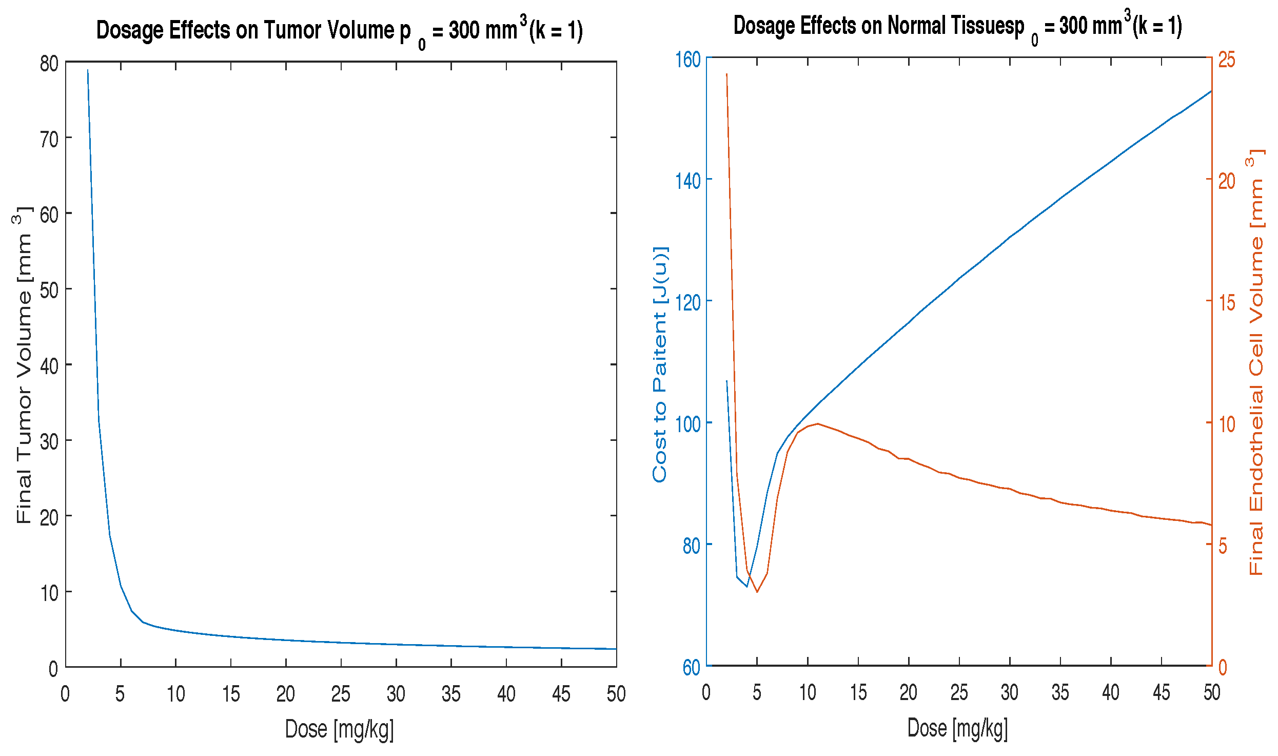
The effect of the dosage of angiogenesis inhibitors was investigated first. Numerical simulations were performed by varying the dosage in 1 mg/kg increments to determine the optimal dosage that minimizes the final tumor volume with a relatively low cost function, . These results are presented in Figure 1.
As can be seen in Figure 1, subjecting the model given by Equations (3) and (4) to our optimal control problem, a continuous optimal control protocol can effectively reduce the volume of the tumor. Since the cost function represents the potential side effects of the drug, it is important to choose the best treatment regimen that minimizes both the tumor cells and the toxicity . Running several simulations we can find the optimal dosage for administering the angiogenesis inhibitors, validating both mathematical parameters proposed in past work and clinical observations reported in medical literature.
This investigation begins with a small value of k (k = 0.1) which signifies low side effects from the administration of the drug. Figure 1 shows that with this continuous model the cost function and the tumor volume can be minimized for all initial tumor volumes. This figure also provides doses of interest for further investigation between 10 mg/kg and 20 mg/kg of drug for all initial conditions considered.
Figure 2 illustrates the effects of implementing optimal control on a case by case basis for the distinct initial values of tumor volume in consideration. The optimal administration of anti-angiogenesis drugs is at full strength for the beginning of treatment and then decays gradually until the end of treatment. The decay happens sooner for higher doses G and lower values of . The fact that the control is a continuous function is in contrast to the “0asa0” results in [33] in which the bang-bang control produced a discontinuous control function.
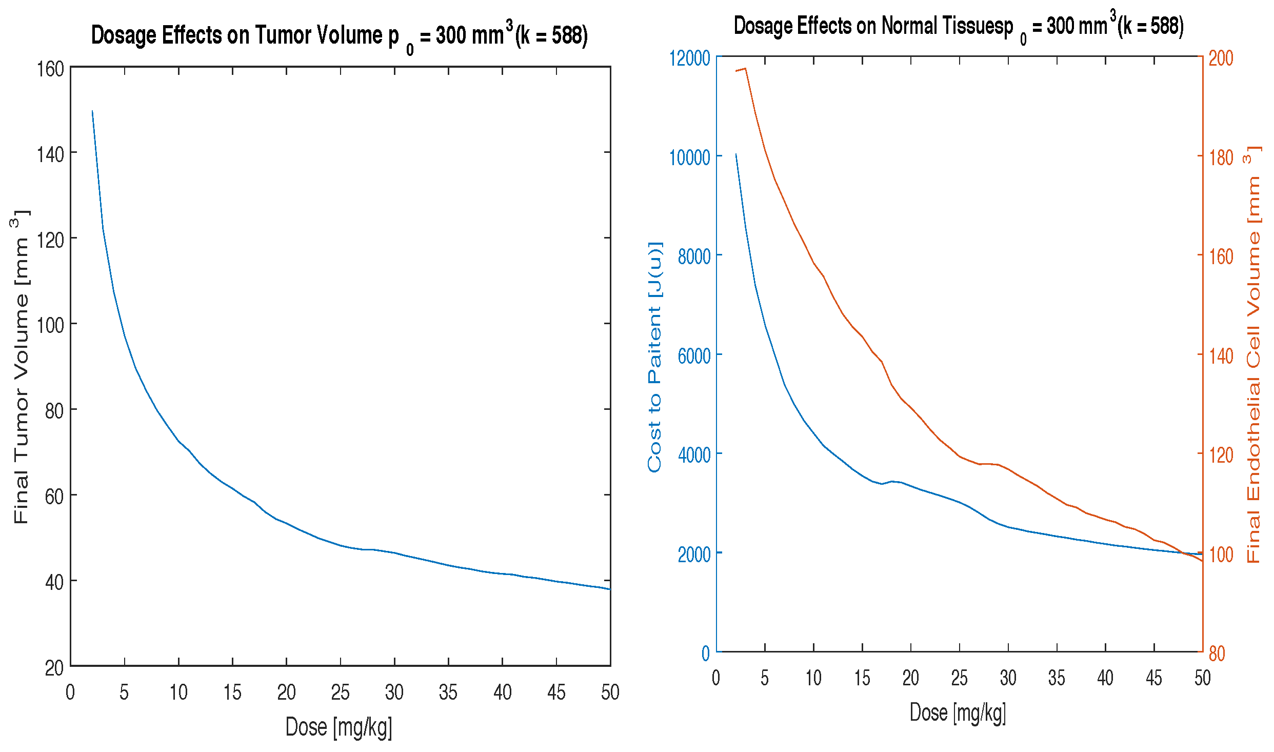
For larger values of k, the results become significantly more complex. Since k is a weighting factor on how much the treatment will negatively effect the patient, it can be assumed that as k increases, the optimal control u will change the dosing scheme to compensate for the increasing negative effects of the drug. The effects of k are investigated by choosing a broad range of values as presented in Table 1. We include a case in which k is a function of , the initial tumor volume, and T, the duration of the study, based on the results found by Garcia et al. [20]. In particular, we use the term as a means to compensate for the observation that fourteen percent of patients receiving angiogenesis inhibitors with their tumor volume were shown to have negative side effects at the end of treatment. The worst case scenario for k (, T = 2 weeks) is shown to illustrate the importance of choosing a meaningful value of k.
Figure 3, Figure 4 and Figure 5 illustrate the effects of varying the parameter k. For a small increase in k (), the cost function and endothelial volume graphs in Figure 3 look similar to that of the case where with the same initial condition given in Figure 1. However, for larger increases in k the cost function and endothelial volume graphs change dramatically. For these cases it can no longer be concluded that the clinically useful range of doses (10–20 mg/kg) is the optimal dosing scheme.
Figure 4 shows that good tumor control can still be obtained using the clinically useful range of 10–20 mg/kg but that the cost to the patient will increase significantly and the patient will experience more severe side effects. In the lower dose range, where the cost function is a minimal, tumor control can be achieved but the volume will not reduce as significantly.
Figure 5, the highest value of k, shows that despite the cost being so high you can still achieve good tumor volume reduction, but you will need a higher dosing scheme to do so. In this case, it makes more sense to use a high dose of 50 mg/kg to eradicate as much of the tumor as possible before the negative side effects take place. In other words, since the cost to the patient is high no matter what the dosing scheme you want to use is going to be, it makes more sense to use a high dose of drug. This is akin to what is done in other cancer therapies, such as radiation, where high doses are given over a short amount of time for patients that are at high risk for negative side effects or at high risk for metastatic disease spreading.
It is important to find the correct value of k to achieve the correct results. k represents the biological side effects of the administered drugs. This is not a fixed value and will change based on the biology of the system, the drug being used, the time-frame of the treatment, and the initial conditions of the tumor volume. Further study into determining the amount of side effects in a specific patient with a specific drug must be done to create a system for evaluating the correct value of k. A database could be created to include the frequency and severity of side effects based on the initial and final conditions. Then correction factors can be determined based on biologically relevant statistics such as age, sex, and other predetermined factors. With this information, the model presented here can be used in a case-by-case basis to optimize the cancer treatment with angiogenesis inhibitors.
4. Conclusions
When discussing any form of treatment for cancer it is important to consider the negative side effects that treatment will have on the patient. The goal of any treatment is to destroy as many cancer cells as possible while limiting toxicity of the treatment to a reasonable minimum. Since developing vasculature is most important to fetus development [42], there are limited side effects to angiogensis therapy for adults. However, there still are side effects as even adults require new vasculature to maintain blood flow to vital organs for oxygen and nutrient transfer.
These results show that in the clinically relevant dosage range of 10–20 mg/kg one can achieve good tumor response with continuous drug concentration while minimizing the toxicity which represents negative side effects of angiogenesis inhibitors by tapering off the concentration at the end of treatment. This is true for all initial tumor volumes and most values of the parameter k.
Figure 3, Figure 4 and Figure 5 show the importance of studying the side effects of anti-angiogenesis therapy from both a biological and mathematical perspective. Doing so will allow physicians to choose the precise value of k that is representative of biological side effects. Further work must be done to determine a biologically relevant range of values of k that take into consideration factors that lead to side effects in patients. Once a method for determining k is created, this model can be used to optimize the treatment of solid tumors with angiogenesis inhibitors on a case-by-case basis.
The work presented in this paper shows that good tumor control can be achieved using a continuous dosing strategy for anti-angiogenesis therapy. The model presented has solved the singularity issue of the bang-bang control model presented in [32] and shown that continuous amounts of anti-angiogenesis drugs in a system reduces tumor volume greatly over a two week time frame. Technology currently exists to administer drugs in such a way that the concentration in blood is at the desired level [43]. These infusion pumps can be used to administer the dosing scheme developed in this paper.
Tumor angiogenesis is a convenient method for tumors to attract endothelial vessels to provide them with the necessary nutrients and oxygen to grow and metastasize. Since all drugs have side effects, it is important to find the optimal timing and dosage to give to a patient to reduce the angiogenesis process as a potential treatment for cancerous tumors. These findings show that given a continuous low dose regimen of angiogensis inhibitors a tumor volume present in a body can be greatly reduced by attacking the endothelial cells, preventing the tumor from receiving the necessary nutrients for survival and growth. While the current practice is to administer angiogensis inhibitors in 1–2 injections per week, given these promising results, perhaps one day the delivery prescription of these drugs will be changed to match what has been simulated, creating one more tool in the fight against cancer.
Acknowledgments
The authors would like to thank the referees for providing valuable comments and suggestions that helped improve the quality of the paper.
Author Contributions
A.E.G. and A.M. contributed equally in the design and implementation of this work, including the writing of the MATLAB code to run the simulations. A.E.G. and A.M. contributed equally to the Background and Results and Discussion sections. A.M. wrote the Methods section. A.E.G. wrote the Conclusion section.
Conflicts of Interest
The authors declare no conflicts of interest.
References
- NIH. Cancer Statistics. National Cancer Institute. National Institute of Health. Available online: https://www.cancer.gov/about-cancer/understanding/statistics (accessed on 4 February 2016).
- Collins, F.S. Testimony on the Fiscal Year 2017 Budget Request before the Senate Committee; National Institutes of Health: Washington, DC, USA, 2016. [Google Scholar]
- Gottesman, M. Mechanisms of cancer drug resistance. Annu. Rev. Med. 2002, 53, 615–627. [Google Scholar] [CrossRef] [PubMed]
- Riesco-Martinez, M.; Parra, K.; Saluja, R.; Francia, G.; Emmenegger, U. Resistance to metronomic chemotherapy and ways to overcome it. Cancer Lett. 2017, 400, 311–318. [Google Scholar] [CrossRef] [PubMed]
- Choi, B.H.; Kwak, M.K. Shadows of NRF2 in cancer: Resistance to chemotherapy. Curr. Opin. Toxicol. 2016, 1, 20–28. [Google Scholar] [CrossRef]
- Fine, H.A.; Dear, K.B.; Loeffler, J.S.; Black, P.M.; Canellos, G.P. Meta-analysis of radiation therapy with and without adjuvant chemotherapy for malignant gliomas in adults. Cancer 1993, 71, 2585–2597. [Google Scholar] [CrossRef]
- Li, L.; Zhao, L.; Lin, B.; Su, H.; Su, M.; Xie, D.; Jin, X.; Xie, C. Adjuvant Therapeutic Modalities Following Three-field Lymph Node Dissection for Stage II/III Esophageal Squamous Cell Carcinoma. J. Cancer 2017, 8, 2051–2059. [Google Scholar] [CrossRef] [PubMed]
- Colliez, F.; Gallez, B.; Jordan, B.F. Assessing Tumor Oxygenation for Predicting Outcome in Radiation Oncology: A Review of Studies Correlating Tumor Hypoxic Status and Outcome in the Preclinical and Clinical Settings. Front. Oncol. 2017, 7, 10. [Google Scholar] [CrossRef] [PubMed]
- Fu, K.K.; Pajak, T.F.; Trotti, A.; Jones, C.U.; Spencer, S.A.; Phillips, T.L.; Garden, A.S.; Ridge, J.A.; Cooper, J.S.; Ang, K.K. A Radiation Therapy Oncology Group (RTOG) phase III randomized study to compare hyperfractionation and two variants of accelerated fractionation to standard fractionation radiotherapy for head and neck squamous cell carcinomas: First report of RTOG 9003. Int. J. Radiat. Oncol. Biol. Phys. 2000, 48, 7–16. [Google Scholar] [CrossRef]
- Al-Abd, A.M.; Alamoudi, A.J.; Abdel-Naim, A.B.; Neamatallah, T.A.; Ashour, O.M. Anti-angiogenic agents for the treatment of solid tumors: Potential pathways, therapy and current strategies—A review. J. Adv. Res. 2017, 8, 591–601. [Google Scholar] [CrossRef] [PubMed]
- Holash, J.; Davis, S.; Papadopoulos, N.; Croll, S.D.; Ho, L.; Russell, M.; Boland, P.; Leidich, R.; Hylton, D.; Burova, E.; et al. VEGF-Trap: A VEGF Blocker with Potent Antitumor Effects. Proc. Natl. Acad. Sci. USA 2002, 99, 11393–11398. [Google Scholar] [CrossRef] [PubMed]
- Bergers, G.; Benjamin, L.E. Tumorigenesis and the angiogenic switch. Nat. Rev. Cancer 2003, 3, 401–410. [Google Scholar] [CrossRef] [PubMed]
- Yoo, M.H.; Hatfield, D.L. The cancer stem cell theory: Is it correct? Mol. Cell. 2008, 26, 514–516. [Google Scholar]
- NIH. Angiogenesis Inhibitors. National Cancer Institute. National Institute of Health. Available online: https://www.cancer.gov/about-cancer/treatment/types/immunotherapy/angiogenesis-inhibitors-fact-sheet (accessed on 4 February 2016).
- Zetter, B.R. Angiogenesis and tumor metastasis. Annu. Rev. Med. 1998, 49, 407–424. [Google Scholar] [CrossRef] [PubMed]
- Elice, F.; Rodeghiero, F. Side effects of anti-angiogenic drugs. Thromb. Res. 2012, 129 (Suppl. 1), S50–S53. [Google Scholar] [CrossRef]
- Thompson, W.D.; Li, W.W.; Maragoudakis, M. The clinical manipulation of angiogenesis: Pathology, side-effects, surprises, and opportunities with novel human therapies. J. Pathol. 2000, 190, 330–337. [Google Scholar] [CrossRef]
- Cook, K.M.; Figg, W.D. Angiogenesis Inhibitors: Current Strategies and Future Prospects. CA: A Cancer J. Clin. 2010, 60, 222–243. [Google Scholar] [CrossRef] [PubMed]
- Jain, R.K.; Duda, D.G.; Clark, J.W.; Loeffler, J.S. Lessons from phase III clinical trials on anti-VEGF therapy for cancer. Nat. Clin. Pract. Oncol. 2006, 3, 24–40. [Google Scholar] [CrossRef] [PubMed]
- Garcia, A.A.; Hirte, H.; Fleming, G.; Yang, D.; Tsao-Wei, D.D.; Roman, L.; Groshen, S.; Swenson, S.; Markland, F.; Gandara, D.; et al. Phase II clinical trial of bevacizumab and low-dose metronomic oral cyclophosphamide in recurrent ovarian cancer: A trial of the California, Chicago, and Princess Margaret Hospital phase II consortia. J. Clin. Oncol. 2008, 26, 76–82. [Google Scholar] [CrossRef] [PubMed]
- Bellomo, N.; Li, N.; Maini, P.K. On the foundations of cancer modelling: Selected topics, speculations, and perspectives. Math. Model. Method Appl. Sci. 2008, 18, 593–646. [Google Scholar] [CrossRef]
- Chaplain, M.A.J.; McDougall, S.R.; Anderson, A.R.A. Mathematical modeling of tumor-induced angiogenesis. Ann. Rev. Biomed. Eng. 2006, 8, 233–257. [Google Scholar] [CrossRef] [PubMed]
- Alarcon, T.; Byrne, H.M.; Maini, P.K. A cellular automaton model for tumour growth in an inhomogeneous environment. J. Theor. Biol. 2003, 225, 257–274. [Google Scholar] [CrossRef]
- Alarcon, T.; Byrne, H.M.; Maini, P.K. A multiple scale model for tumor growth. Multiscale Model. Simul. 2005, 3, 440–475. [Google Scholar] [CrossRef] [Green Version]
- Spill, F.; Guerrero, P.; Alarcon, T.; Maini, P.K.; Byrne, H.M. Mesoscopic and continuum modelling of angiogenesis. J. Math. Biol. 2014, 70, 485–532. [Google Scholar] [CrossRef] [PubMed]
- Hahnfeldt, P.; Panigrahy, D.; Folkman, J.; Hlatky, L.R. Tumor development under angiogenic signaling: A dynamical theory of tumor growth, treatment response, and postvascular dormancy. Cancer Res. 1999, 59, 4770–4775. [Google Scholar]
- Sachs, R.K.; Hlatky, L.R.; Hahnfeldt, P. Simple ODE models of tumor growth and anti-angiogenic or radiation treatment. Math. Comput. Model. 2001, 33, 1297–1305. [Google Scholar] [CrossRef]
- Ergun, A.; Camphausen, K.; Wein, L.M. Optimal scheduling of radiotherapy and angiogenic inhibitors. Bull. Math. Biol. 2003, 65, 407–424. [Google Scholar] [CrossRef]
- Norton, L.; Simon, R. Tumor size, sensitivity to therapy, and design of treatment schedules. Cancer Treat. Rep. 1997, 61, 1307–1317. [Google Scholar]
- Norton, L.; Simon, R. The Norton—Simon hypothesis revisited. Cancer Treat. Rep. 1986, 70, 163–169. [Google Scholar] [PubMed]
- D’Onofrio, A.; Gandolfi, A. Tumour eradication by antiangiogenic therapy: Analysis and extensions of the model by Hahnfeldt et al. (1999). Math. Biosci. 2004, 191, 159–184. [Google Scholar]
- Ledzewicz, U.; Schättler, H. A synthesis of optimal controls for a model of tumor growth under angiogenic inhibitors. In Proceedings of the 44th IEEE Conference on Decision and Control, Sevilla, Spain, 12–15 December 2005; pp. 934–939. [Google Scholar]
- Ledzewicz, U.; Schättler, H. Anti-angiogenic therapy in cancer treatment as an optimal control problem. SIAM J. Control Optim. 2007, 46, 1052–1079. [Google Scholar] [CrossRef]
- Nilsson, F.; Kosmehl, H.; Zardi, L.; Neri, D. Targeted delivery of tissue factor to the ED-B domain of fibronectin, a marker of angiogenesis, mediates the infarction of solid tumors in mice. Cancer Res. 2001, 61, 711–716. [Google Scholar] [PubMed]
- D’Onofrio, A.; Gandolfi, A.; Rocca, A. The dynamics of tumour-vasculature interaction suggests low-dose, time-dense anti-angiogenic schedulings. Cell Prolif. 2009, 42, 317–329. [Google Scholar] [CrossRef] [PubMed]
- Fleming, W.H.; Rishel, R.W. Deterministic and Stochastic Optimal Control; Springer: New York, NY, USA, 1975. [Google Scholar]
- Pontryagin, L.S.; Boltyanskii, V.G.; Gamkrelidze, R.V.; Mishchenko, E.F. The Mathematical Theory of Optimal Processes; Wiley: New York, NY, USA, 1962. [Google Scholar]
- Goldman, C.K.; Kendall, R.L.; Cabrera, G.; Soroceanu, L.; Heike, Y.; Gillespie, G.Y.; Siegal, G.P.; Mao, X.; Bett, A.J.; Huckle, W.R.; et al. Paracrine expression of a native soluble vascular endothelial growth factor receptor inhibits tumor growth, metastasis, and mortality rate. Proc. Natl. Acad. Sci. USA 1998, 95, 8795–8800. [Google Scholar] [CrossRef] [PubMed]
- Klement, G.; Baruchel, S.; Rak, J.; Man, S.; Clark, K.; Hicklin, D.J.; Bohlen, P.; Kerbel, R.S. Continuous Low-dose Therapy with Vinblastine and VEGF Receptor-2 Antibody Induces Sustained Tumor Regression without Overt Toxicity. J. Clin. Investig. 2000, 105, R15. [Google Scholar] [CrossRef] [PubMed]
- Shih, T.; Lindley, C. Bevacizumab: An angiogenesis inhibitor for the treatment of solid malignancies. Clin. Ther. 2006, 28, 1779–1802. [Google Scholar] [CrossRef] [PubMed]
- Lenhart, S.; Workman, J.T. Optimal Control Applied to Biological Models; CRC Press: New York, NY, USA, 2007. [Google Scholar]
- Zygmunt, M.; Herr, F.; Münstedt, K.; Lang, U.; Liang, O.D. Angiogenesis and vasculogenesis in pregnancy. Eur. J. Obstet. Gynecol. Reprod. Biol. 2003, 110, S10–S18. [Google Scholar] [CrossRef]
- Center for Devices and Radiological Health. Infusion Pumps—What Is an Infusion Pump? U.S. Food and Drug Administration Home Page, Center for Devices and Radiological Health: Silver Spring, MD, USA, 2014.
Figure 1.
Results using various initial conditions, , and time t = 2 weeks.
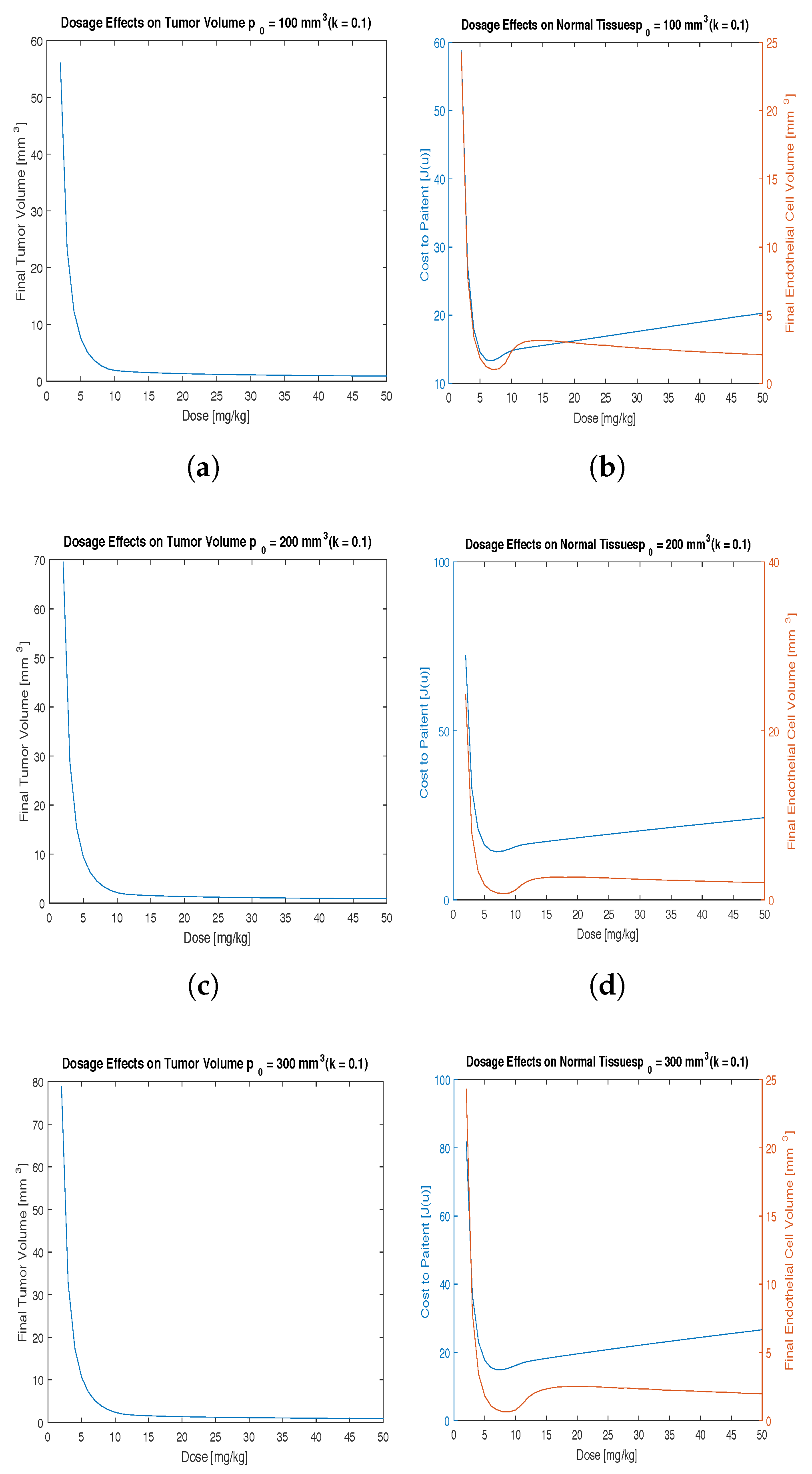
Figure 2.
Results using initial conditions (a) = 100 mm, (b) 200 mm, (c) 300 mm and time t = 2 weeks.
Figure 2.
Results using initial conditions (a) = 100 mm, (b) 200 mm, (c) 300 mm and time t = 2 weeks.
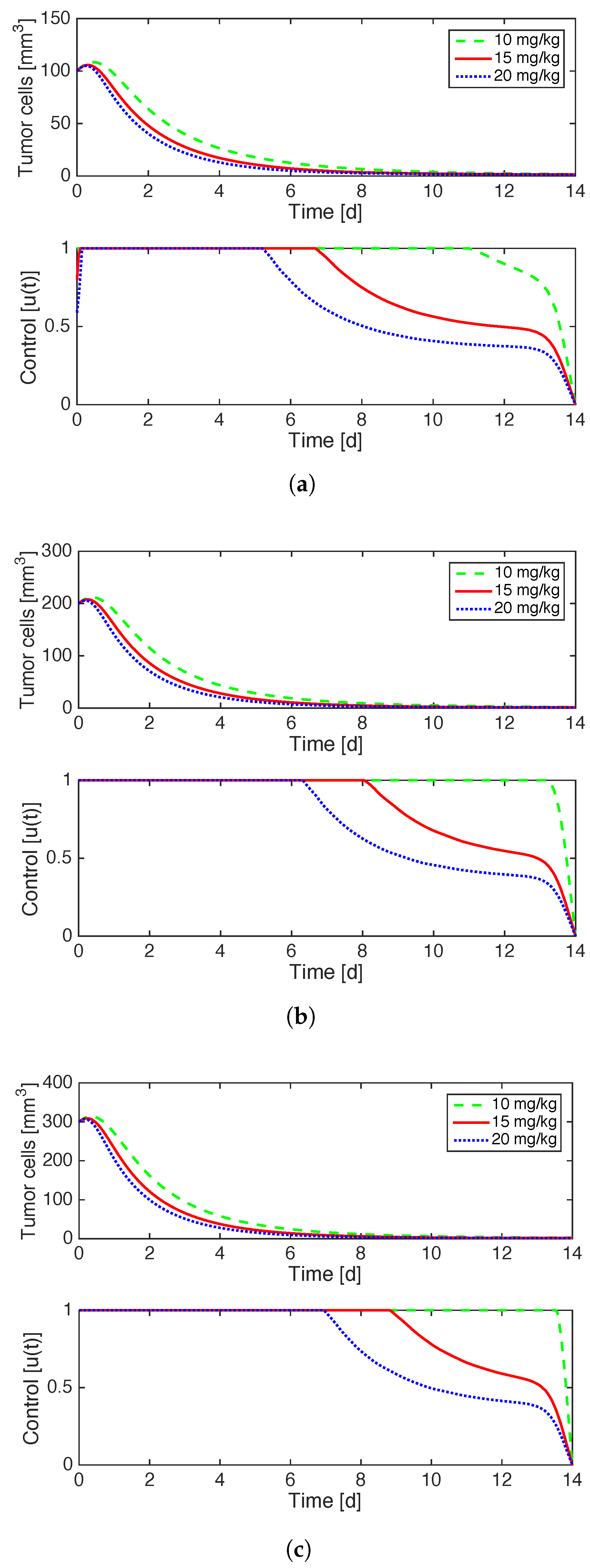
Figure 3.
Results using , mmd, and time t = 2 weeks.

Figure 4.
Results using , mmd, and time t = 2 weeks.
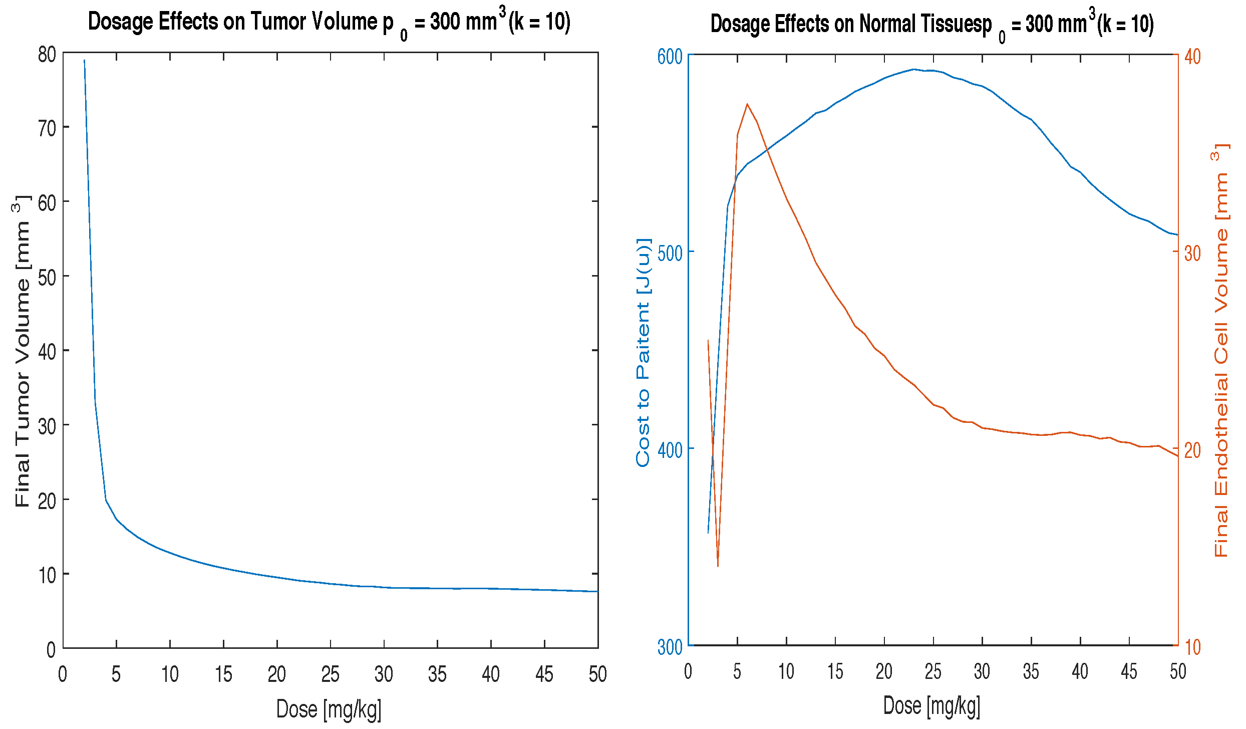
Figure 5.
Results using , mmd, and time t = 2 weeks.

Table 1.
Description and value of all relevant parameters.
| Parameter | Description | Value |
|---|---|---|
| Tumor Growth Parameter | per day | |
| b | Endothelial Stimulation Parameter | 5.85 mm per day |
| d | Endothelial Inhibition Parameter | 0.00873 per mm per day |
| T | Time frame of Study | 14 days |
| G | Prescription Dose | 2–50 |
| Prescription Dose Investigated | 10 | |
| 15 | ||
| 20 | ||
| k | Toxicity Parameter | 0.1 mmday |
| 1 mmday | ||
| 10 mmday | ||
| mmday |
© 2017 by the authors. Licensee MDPI, Basel, Switzerland. This article is an open access article distributed under the terms and conditions of the Creative Commons Attribution (CC BY) license (http://creativecommons.org/licenses/by/4.0/).
Share and Cite
MDPI and ACS Style
Glick, A.E.; Mastroberardino, A. An Optimal Control Approach for the Treatment of Solid Tumors with Angiogenesis Inhibitors. Mathematics 2017, 5, 49. https://doi.org/10.3390/math5040049
AMA Style
Glick AE, Mastroberardino A. An Optimal Control Approach for the Treatment of Solid Tumors with Angiogenesis Inhibitors. Mathematics. 2017; 5(4):49. https://doi.org/10.3390/math5040049
Chicago/Turabian StyleGlick, Adam E., and Antonio Mastroberardino. 2017. "An Optimal Control Approach for the Treatment of Solid Tumors with Angiogenesis Inhibitors" Mathematics 5, no. 4: 49. https://doi.org/10.3390/math5040049
Note that from the first issue of 2016, this journal uses article numbers instead of page numbers. See further details here.