
Dynamics of Amoebiasis Transmission: Stability and Sensitivity Analysis

1
Department of Mathematics, Faculty of Science, Jain University, Bangalore, Karnataka 560041, India
2
Department of Computer Science and Engineering, Center for Applied Mathematical Modeling and Simulation (CAMMS), P.E.S. Institute of Technology-Bangalore South Campus (PESIT-BSC), Bangalore, Karnataka 560100, India
3
Department of Basic Sciences, School of Engineering and Technology, Jain University (Global Campus), Kanakapura, Karnataka 562112, India
*
Authors to whom correspondence should be addressed.
†
Current address: University of Gitwe, Bweramana, Southern Province, P.O Box 1 Nyanza, Rwanda.
Mathematics 2017, 5(4), 58; https://doi.org/10.3390/math5040058
Submission received: 8 August 2017
/
Revised: 19 September 2017
/
Accepted: 24 September 2017
/
Published: 1 November 2017
Abstract
:Compartmental epidemic models are intriguing in the sense that the generic model may explain different kinds of infectious diseases with minor modifications. However, there may exist some ailments that may not fit the generic capsule. Amoebiasis is one such example where transmission through the population demands a more detailed and sophisticated approach, both mathematical and numerical. The manuscript engages in a deep analytical study of the compartmental epidemic model; susceptible-exposed-infectious-carrier-recovered-susceptible (SEICRS), formulated for Amoebiasis. We have shown that the model allows the single disease-free equilibrium (DFE) state if , the basic reproduction number, is less than unity and the unique endemic equilibrium (EE) state if is greater than unity. Furthermore, the basic reproduction number depends uniquely on the input parameters and constitutes a key threshold indicator to portray the general trends of the dynamics of Amoebiasis transmission. We have also shown that is highly sensitive to the changes in values of the direct transmission rate in contrast to the change in values of the rate of transfer from latent infection to the infectious state. Using the Routh–Hurwitz criterion and Lyapunov direct method, we have proven the conditions for the disease-free equilibrium and the endemic equilibrium states to be locally and globally asymptotically stable. In other words, the conditions for Amoebiasis “die-out” and “infection propagation” are presented.
1. Introduction
Entamoeba histolytica causes Amoebiases, which is counted among a group of chronic, disabling and disfiguring diseases, known as the Neglected Tropical Diseases (NTDs). NTDs affect some disadvantaged urban populations where the conditions of sanitation are not favorable and have a degrading effect on the poor. According to a 2009 World Bank report, 51% of the population of Sub-Saharan Africa (SSA) lives on less than U.S. $1.25 per day, and 73% of the same population lives on less than U.S. $2 per day [1]. The underprivileged economic status coupled with congested neighborhoods and exploding birth rates contribute to the wide spread of Entamoeba histolytica among this population. The adverse effects of NTDs on child development, pregnancy outcome and agricultural productivity have forced 500 million people in SSA to live in permanent conditions of poverty [1]. In SSA, the epidemiology of Amoebiasis is not clearly understood because of limited research done on the subject. The lack of modern diagnostic techniques does not allow differentiating between the infections resulting from the two morphologically-identical strains, Entamoeba histolytica and Entamoeba dispar. However, the overall distribution in prevalence of Amoebiasis is believed to be high in SSA. Sudan, Cote D’Ivoire, Nigeria, Egypt and South Africa are among these countries. As an example, a study was conducted assessing the presence of Entamoeba strains, on the stool and sero-prevalence of children in two regions of South Africa. This study came out with a disparate result in rates of prevalence among two different communities; the region supplied with clean water reported a meager 2% in prevalence, while a rural region with a few sources of water reported prevalence of more than 50% [2]. Apart from SSA, Amoebiasis is a disease that is generally frequent in developing countries like India, Bangladesh, Mexico and Japan [3]. However, rare cases are reported in developed countries like the USA and Europe (England) [4].
Amoebiasis is generally triggered by the ingestion of food or beverage contaminated by the infective cysts of Entamoeba histolytica. The infection, on reaching the large intestine, ex-cyst, multiplies by cellular divisions, becoming invasive trophozoites [5]. The onset of Amoebiasis takes place when the trophozoites degrade and invade the mucus protection of the intestinal wall and start to destroy intestine cells. The massive killing of intestinal cells degenerates subsequently into inflammation yielding to dysentery [6]. Five percent of these cases may exhibit extra-intestinal Amoebiasis; especially Amoebic liver abscess (ALA) after a period of 1–3 months. Statistical reports show that 90% of the prevalence of Entamoeba histolytica infection is typically asymptomatic (i.e., here referred to as carriers), and the remaining 10% are in a state of acute infections [7,8]. Thibeaux et al.’s research agrees on the predominant asymptomatic nature of amoebic infections; since 20% of them result in intestinal Amoebiasis [6]. In some developing countries, age seems to be a risk factor for Amoebiasis. The young, under 15 years old, were more likely to be infected than the other age groups, and children between the age of five and nine years old were the most affected [9]; although, research is yet to confirm this. In the United States of America, children and adults of both genders are equally affected by Amoebiasis [10], even though some data and anecdotal evidence suggest a male predominance [11,12]. The prevalence may change seasonally, and there appears to be both acquisition and loss of the infection throughout the year [3]. Moreover, Caballero-Salcedo A. et al. [13] and Samie et al. [11] have indicated that, in developing countries, individuals are often exposed to Entamoeba histolytica, making serological tests incapable of distinguishing past infection from current infection [11] in a definitive manner. Individuals with human immunodeficiency virus (HIV) and acquired immune deficiency syndrome (AIDS) belong to a category of people who could be at risk of Entamoeba histolytica and may possibly develop one of the three kinds of Amoebiasis mentioned earlier [9,10,12]. Furthermore, an increased risk of Amoebiasis among men who have sex with men (MSM) has been reported in East Asian countries such as Japan, Taiwan and South Korea [2]. It is well documented that men in Africa are most vulnerable to Amoebiasis infections due to their continuous travel in search of financial support for their families. In South Africa and some other countries, the risk factor for ALA is observed to be greater among men; approximately 10-times more than among women [10]. As a matter of fact, 83% of the reported cases in South Africa are men [2]. Thus, pathological conditions of Amoebiasis may vary with diverse factors, some of which are environmental conditions, sexually-transmitted diseases (syphilis), social behavior and economic status of the population.
1.1. Diagnosis of Amoebiasis
The diagnosis and detection of Entamoeba histolytica prove to be challenging tasks, which produce results that are occasionally correct. Microscopy diagnosis of Entamoeba histolytica requires diligent methods and procedures, which are prone to erroneous interpretation. The presence of two morphologically-confusing strains [14] within a sample of stool remains the major problem for optical microscope-based exams. Using microscopy for Amoebiasis diagnosis was declared inefficient by World Health Organization (WHO) in 1997 [14]. This method has become obsolete since the introduction of the new diagnostic approach based on antigen detection tests for Entamoeba histolytica. In different parts of the world, there are modern methods and procedures based on the culture of the trophozoites complemented by iso-enzyme analysis such as enzyme-linked immunosorbent assay (ELISA)These methods allow one to distinguish the infections from the two identical strains. Another laboratory diagnosis of Amoebiasis is based on antibody detection. Stool IgA antilectin antibodies and serum IgG antilectin antibodies are the kinds of antibodies used to diagnose the prior and current Entamoeba histolytica infections. However, WHO has made the decision to replace diagnosis based on microscopy by the Tech Lab (Blacksburg, VA) Entamoeba histolytica stool antigen detection test [14,15]. This was done because other diagnoses based on other antigen detection tests are still questionable as they react with Entamoeba dispar.
It is important to highlight some findings resulting from the use of any diagnosis method: Entamoeba dispar is more prevalent in number than Entamoeba histolytica. Lawson et al. [14] have found Entamoeba histolytica and Entamoeba dispar in respective proportions of 1% and 13% of the stool samples examined in Brazil [14]. A study of asymptomatic cases conducted by Dhawan et al. [12] on Amoebiasis in the United States of America has confirmed the estimated prevalence of Entamoeba dispar to be 10-times more than that of Entamoeba histolytica [12]. These two studies generalize the tendency for the prevalence of dispar in developed countries. However, in most developing countries, Entamoeba dispar is three-times more common than Entamoeba histolytica [10]. Yet, few exceptions are noticeable, i.e., the study conducted in Egypt in the rural area of Kafer Daoud by ELISA revealed the prevalence rate of 21.4% for Entamoeba histolytica and 24.2% for Entamoeba dispar. In this area, the prevalence of both species of Entamoeba presents a slight difference [2].
1.2. Immunity and Vaccine
The onset of the disease raises many questions including the post-disease health consequences. For this reason, it is very fundamental to know whether a patient who has recovered from Amoebiasis would acquire induced immunity in the short or long term, against subsequent infections. In the early years of investigation, there was no illumination on this matter. However, the patterns of immune response to the infection and invasion by Entamoeba histolytica came to light in the 20th century. Nowadays, it is known that Amoebiasis induces immunity to the recovered individuals. It has been observed that the patient continues to present a positive serological test for some years after recovery from the disease [10]. A study conducted in Durban, South Africa by Stauffer et al. reported that anti-amoebic antibodies last for at most five years [2]. However, screening 42 children in area of Dhaka, Haque et al. elucidated that newly infected children develop stool IgA antilectin antibodies for a relatively short duration [7]. Levels of these antibodies remained detectable for a mean period of 17 days [16] even though they may not serve as indicators of antibody protective efficacy [15]. On basis of the prevalence of 4 vs. 24% in subsequent Entamoeba dispar infections, Stauffer et al. suggested that patients might develop partial immunity against consecutive Entamoeba dispar infections over a period of three years [2]. Evidently, recuperation from Amoebiasis induces a temporarily-induced immunity.
The remainder of the paper is organized as follows: Section 2 presents a comprehensive outlook on the formulation of the mathematical model bridging the gaps in the literature review of Amoebiasis spread. Section 3 is dedicated to discovering the steady states of Amoebiasis and the threshold parameter for the spread of Amoebiasis. This forms the foundation for the stability analysis of the model. Section 4 is devoted to applying analytical results to the numerical solution and simulations. The authors conclude by setting up some guidelines in terms of prediction, prevention and management of Amoebiasis.
2. Related Work
The mathematical model for the transmission of Amoebiasis through a single population was formulated for the first time by Hategekimana et al. in their paper [17]. As there was no existing mathematical model for Amoebiasis in the literature of mathematical modeling, the initial value problem governing the dynamic transmission of Amoebiasis has been derived by basing the model assumptions on published research. Research used in the modeling was done in clinical, medical and other fields related with Entamoeba histolytica. In referral classical epidemiological models, the population targeted by the study is classified into epidemiological classes or compartments [18,19,20,21]. For Amoebiasis, the population is subdivided into five epidemiological classes or states: susceptible, exposed, infectious, carriers and removal or recovered. Their respective time-dependent sizes as a fraction of the population are denoted by S, E, I, C and R, respectively. Every member of the population may be found in only one of these five epidemiological compartments, and the transfer of people from one compartment to another is subject to the principle of mass action. The Amoebiasis transmission model relies on the following assumptions:
- The infection spreads by means of direct contact between the susceptible with the infectious or carrier in a homogeneously-mixed population. (redDirect contact happens when susceptible people ingest cysts of Entamoeba histolytica contained in water or food infected by human feces).
- The period of the Amoebiasis investigation is relatively extended over a short time scale to maintain an equal balancing birth and natural death rates , and hence, the size of the population under study remains constant during the said period.
- The rate at which susceptible members are infected is proportional to the force of infection , which is a function of transmission and the fraction of the infectious and the carriers i.e., .
Remark 1.
The five epidemiological compartments of Amoebiasis are defined as:
- Susceptible (S): This is the class of individuals who are not yet infected, but can become infected once they are in contact with contaminated food or drink.
- Exposed (E): The class of individuals who are already infected, but not yet able to diffuse cysts in the environment.
- Infectious (I): This class encompasses the individuals infected in the acute stage of the disease, shedding a much greater number of cysts and trophozoites in a mixture of mild stools of blood and mucus.
- Carrier (C): This is the class of people who are asymptomatic to the disease although shedding cysts occasionally.
- Removal (R): This is a class of individuals who recovered from Amoebiasis.
Remark 2.
Briefly, for an adequate number of times that a person is in contact with infected feces of another person, that person catches the infection and progresses to the exposed compartment of the disease at the rate proportional to the size of the susceptible compartment. In other words, the fraction of the population transferred to the exposed compartment from the susceptible compartment per unit of time is equal to . Subsequently, as , the fraction of the population per unit of time in the exposed compartment, become infectious, they leave this compartment to enter the acute compartment. The transfer of the population from one compartment to another does not culminate. Rather, the process continues, and the population amounting to leave the acute compartment and enter the carrier and recovered compartments at respective rates of and . Rarely, some people in the carrier compartment should recover and leave this compartment at a rate of to be located in the recovered compartment. The cycle of the transfer of the population in compartments ends when people in the recovered compartment lose their temporarily-induced immunity from Amoebiasis and return to the susceptible compartment at a rate equivalent to . Note that every person in each compartment may suffer from natural death at a rate proportional to μ, and the susceptible compartment increases in size by the recruited fraction of people equivalent to μ, as well. The variations in the size of the epidemiological compartments per unit of time are finally defined as the consequence of these kinds of transfers.
With the above model assumptions, the initial value problem governing the dynamics of Amoebiasis through a single population is written as:
The initial conditions are as follows:
The parameters used in this model are all positive, and their values range between zero and one. The following Table 1 lists out the parameters used in our model.
Remark 3.
Depending on the values of the parameters,SEICRS epidemic model can be reduced to the SEIRS epidemic model, provided that the acute infectious class, I, and infectious carrier class, C, are combined to give only one class of infectious people, I. The same model may work if the mean time period an individual stays as a carrier of cysts is excessively long (infinite); however, this never happens in the case of Amoebiasis. For this reason, the two infectious states, I and C, have to be considered as two different components of the model. The complete stool analysis exams provide the results based on the presence of cysts (here referred to as the carrier class C) and trophozoites (in reference to the acute infectious class I) separately at some diagnosis centers [22]. This fact supports our assumptions about the distinction between the two classes I and C.
Let the general form of the initial value Problem (IVP) (1)–(6) be represented as:
with x as a time-dependent vector defined by The initial value Problem (IVP) (7) is defined on the domain , which is the Banach space equipped with the metric ; where is the time interval of the course of Amoebiasis. The domain over which the initial value problem (IVP) is defined is as follows:
In their work, Hategekimana et al. [17] focused on the formulation of the model and studied its well-posedness. red(The authors recommend that the readers would refer to the paper [17] for further details of the model. It is easy to verify that there is little overlap between the two papers. Nonetheless, the entire mathematical analysis concerning the stability and sensitivity of the model is novel.). However, they did not study the model analytically. It is for this reason that we have decided to study analytically and numerically the model by writing this paper. The authors believe that their contribution will yield conclusive results related to the general trend of the dynamics of Amoebiasis transmission through the population.
3. Stability Analysis of the Model
We begin by proving the invariance of the domain (8) under the IVP (7). This is conclusive evidence that the solution of the model remains inside the domain of the initial value Problem (7) at any time during the course of Amoebiasis.
Theorem 1.
Ω is positively invariant under the initial value problem (7).
Proof of Theorem 1.
By Equation (8), the domain of the initial value problem (7) is closed, and hence, it is a compact set. Let us mimic the method developed in [18] by considering the boundary of the domain as the union of its subsets expressed as where:
and
For , define the outer normals , where:
and , with:
According to [23,24], is positively invariant under Equation (7) if, for each point x of the boundary, the vector is either a tangent or inward directed. By virtue of the inner product, it is very easy to conclude the invariance of the domain,
for some , and for all i = 1, 2, 3, 4.
Thus, every solution of the initial value problem, which starts inside or on the boundary of the domain , will never cross the domain during the course of moebiasis. ☐
3.1. Threshold Parameters of the Model
The most important aspect in the study of the dynamics of the disease is to quantify the capability of disease transmission through the population. In other words, some conditions described by the threshold parameters have to be fulfilled to invade the population. According to the literature of infectious diseases, the basic reproduction number is the key parameter and it is defined as the number of individuals infected by only one infectious member introduced into the entire population of the susceptible individuals [19,20,21,25,26]. However, in epidemiology modeling, there are other threshold parameters that are too important to be ignored; these are the effective reproduction rate R, the mean age of infection A and the herd immunity threshold . As far as the Amoebiasis’ basic reproduction number is concerned, the onset of Amoebiasis is guaranteed only if one such infectious individual can pass on the disease at an average of at least one susceptible entity. Otherwise, the disease will die out [26]. Indeed, the analytic theory of the dynamics of Amoebiasis is closely associated with the steady states of the dynamics, namely DFE and the endemic equilibrium state.
3.1.1. The Disease-Free Equilibrium State of Amoebiasis
DFE is defined as a constant solution of the initial value problem, for which there is no variation in fractions of the population in each of the four epidemiological components. This state occurs when the population is free from the disease. In other words, DEF is the point of that satisfies the initial value problem (7) restricted to the conditions:
It is easy to see that .
3.1.2. The Basic Reproduction Number
The basic reproduction number of this model is determined by applying the next generation operator, a method derived from the theory of the center manifold and developed by P.van den Driessche and J. Watmough (2002) [25,27,28]. P. van den Driessche’s method for computing the basic reproduction number is based on the rate of change in composition of the infectious classes E, I and C. For this reason, we rewrite Equations (2) to (4) in the form of a vector equation:
where the variable and , while the vector functions and are defined as the flow-rates from non-infected class Y to the infected classes X and the negative of all other flow-rates entering the compartments X, respectively.
The corresponding Jacobian matrices F and V at are given by:
and:
Since the basic reproduction number is equal to the spectral radius of the next generation matrix , i.e., , it follows that,
3.1.3. Endemic Equilibrium State
During the course of Amoebiasis, it may happen that the exiting and entering proportions of individuals in each compartment are balanced. Therefore, there should not be any change in the size of the five epidemiological compartments. At this stage, the Amoebiasis becomes a persistent disease. The endemic equilibrium of Amoebiasis is the point O = of , that satisfies with at least , , different from zero.
Theorem 2.
Amoebiasis persists only if the basic reproduction number is greater than one. Persistence implies that the fraction of susceptible individuals is equal to the reciprocal of the basic reproduction number.
Proof of Theorem 2.
Applying the condition of endemic steady state to Equation (7), we obtain the following solution in the components:
where .
From Equation (20), it is clear that and are the common factors in Equations (18), (19) and (21). Let us assume that the endemic steady state settles down when the basic reproduction is less than one. It follows that and , and are negative, and this does not biologically make sense. Hence the contradiction and the end of the Proof of the Theorem 2. ☐
3.2. Stability Analysis of the Steady States and Sensitivity Analysis
3.2.1. The Stability of the Disease-Free Equilibrium
Theorem 3.
DFE is locally asymptotically stable if the basic reproduction number is less than one and is unstable otherwise.
Proof of Theorem 3.
DFE is asymptotically stable if the real part of all eigenvalues of the matrix is negative; otherwise, DFE is unstable red(the condition for instability follows trivially if the basic reproduction number is greater than or equal to one) [26,29,30].
The characteristic polynomial of the matrix A is then given by:
where , , and are all positive. It is clear that one root of the characteristic polynomial is negative, . Other roots are zeros of the cubic polynomial:
To verify the signs of the real parts of the roots of the polynomial (23), we shall make use of the Routh–Hurwitz test [24,31,32]. According to this test, the real parts of the roots of the cubic polynomial are negative if the coefficients of this polynomial satisfy the following four conditions:
By the definition of the c’s coefficients, the inequality (24) holds true, and the remaining conditions follow from the following proofs:
- Given , it follows that . Hence, . This proves Condition (26).
- We need to show that if , then . Given,but,we obtain:Develop the right side of the inequality by applying the distributive law and the second term to yield the following:Hence, we obtain
As a result of the proof of this theorem, when the basic reproduction number is less than one, the characteristic polynomial Equation (22) has four roots whose real parts are all negative. For this reason, DFE is locally asymptotically stable. ☐
Theorem 4.
The disease-free equilibrium is globally asymptotically stable if the basic reproduction number .
Proof of Theorem 4.
For the stability of DFE, the sizes of the fractions of infective classes E, I and C are continuously decreasing and then settle down at zero during the entire period of the course of the disease. For this reason, any Lyapunov function that involves these sizes has to decrease during the period of the stability. By this fact, as in papers [33,34,35,36], consider that the following Lyapunov function:
is negative if the following three conditions hold true:
and:
Using Equations (30) and (31), the left side of Inequality (32) becomes:
Remark that,
The right hand of Inequality (34) is negative if and only if , that is if , and hence, for all in if . As DFE is the only element in that satisfies , it follows that the largest subset of that satisfies contains only DFE. The global asymptotic stability of DFE follows the LaSalle invariance principle [30]. ☐
3.2.2. Stability of the Endemic Equilibrium
Theorem 5.
Proof of Theorem 5.
Consider the following Lyapunov functional:
where , , and are some strict positive real numbers [24,30,37] to allow the function V to be positive definite on . Differentiating the function V along the solution curve of the IVP Equation (7), we have:
For the remainder of the proof, we need only to show that the above four conditions (39) to (42) hold true as long as for .
Let us assume , and Equation (39) follows.
Now, by the same assumption, the left hand of Equation (40) becomes:
only if and , the proof of Equation (40).
Further, Equation (41) holds that and .
Proof:
It is clear that the inequality holds only if , as in this case, and
As far as the condition (42) is concerned, by developing the left side of the corresponding inequality and using (18) and (19) by the fact that is much smaller than , we have:
It follows that the inequality holds only for .
From the proofs of the above four conditions, it follows that for any strictly positive real numbers that satisfy the condition , the derivative is negative definite on and only at the endemic equilibrium point . Thus, the asymptotic stability of the endemic equilibrium point follows from LaSalle’s invariance principle [30]. ☐
By the property of the asymptotic stability of both DFE point and the endemic equilibrium point of Amoebiasis, we deduced the manner in which Amoebiasis will disappear or persist in the population. Depending on the number of susceptible people infected by a single infectious individual and in view of the global asymptotic stability of the said steady states, there is maximum assurance that Amoebiasis will cease to propagate and disappear completely if the average number of these people infected by only one infectious patient is less than one. This would happen regardless of the fraction of people initially infected in a given population. On the contrary, if the number of people who acquired the infection from one infectious individual is greater than one, then Amoebiasis will certainly be a persistent disease in the population.
In the next section, we will discuss the numerical solution of the proposed model and the consequences of such an exercise.
3.3. Sensitivity Analysis
This section discusses the impact of the change in values of the parameters on the functional value of the basic reproduction number . According to the definition provided by Chitnis et al. [38] and reading [28], the normalized forward sensitivity index of the basic reproduction number to the parameter, say P, of the epidemic model is denoted by and defined as:
This is the ratio of the relative change in the basic reproduction number to the relative change in the values of the concerned parameter. As a consequence of this definition, let and represent n infinitesimal amount of changes in parameter P and in basic reproduction number , respectively, then the sensitivity index of related to the parameter P can be expressed as:
According to Equation (47), we conclude that there is a relative change in the basic reproduction value equal to % resulting from the relative change (either increasing or decreasing) % in the value of the parameter P.
Below are algebraic expressions of the sensitivity index of to the parameter P, where P stands for :
As the disease transmission possibility depends on the value of the basic reproduction number, it is very important to know which parameters play a key role in variations of the basic reproduction number. In other words, these parameters serve as a feature tool and guide to health managers as they are designing policy for the control of Amoebiasis spread. Inspecting the expected value of sensitivity indices of provided by Equation (48) to Equation (54), we clearly see that the most influential parameter in terms of the change of values of the basic reproduction number is the direct transmission rate . The maximum absolute value of the sensitivity index of to the parameters is one, and it is achieved to the parameter ; and the smallest absolute value of the sensitivity of occurs for the parameter . Note that for other parameters, the sensitivity indices of the basic reproduction number vary over the interval .
The importance of the epidemic model is to establish the conditions for an efficient control of the spread of infections and to predict the epidemic population-levels of the dynamics of the disease during the course of the disease. The disease control is efficient when its effects undermine the transfer of individuals from susceptible to infectious epidemic compartments. These two major targets of the epidemic model are often subject to the parameters of the model. A simple change in values of one or more parameters of the disease could yield sensitive consequences on the capability of the disease to spread. As the normalized forward sensitivity is a tool for analyzing such trends in the dynamics of disease transmission, the authors of this paper have opted to analyze the model based on this kind of sensitivity. Our goal was to find the most influential parameters or the key parameters for the variation in the values of the threshold parameter, , for the spread of Amoebiasis. Once they are known, health policy makers may deal with them for intervention strategies. The authors suppose the change in the key parameters to be explicative cause of the tightness observed in the numerical simulation part of this article. For example, the piles of solution curves seen in Figure 1b, Figure 2b and Figure 3b are produced from only one solution curve. By initiating a small change in the value of every parameter involved in IVP of the model 25 times, we realized that every change in the value of these parameters brings forth a new solution curve starting from the same initial value. Furthermore, twenty five solution curves resulting from this simulation procedure are more tightened for the value of the basic reproduction number less than unity and progressively lose their tightness for the value of the basic reproduction number greater than unity. This phenomenon is eloquently explained by the general application of the normalized forward sensitivity of the basic reproduction number to the parameters of the model.
4. Numerical Solution and Simulation
The patterns in the dynamics of Amoebiasis transmission are entirely characterized by , the basic reproduction number. The basic reproduction number, as shown in Section 3, is the threshold parameter for the stability of the two steady states in the proposed mathematical model. It is also a useful parameter to study in the context of sensitivity analysis of the model. depends only on the input (parameters). For the sake of agreement between analytical and numerical results, it is necessary to explore the general behavior of the numerical solutions as the values of the parameters change. Reasonably, the influence of changes in parametric values may explain the true behavior of the dynamics of Amoebiasis transmission. The study is relevant since it is known that the parameters in question may vary seasonally or geographically.
In order to find out the values that the parameter (used in the model) may assume suitably, the authors refer to Haque et al. [7] and other sources. For instance, the following has been discovered in regard to the value of the parameters:
- Abd-Alla et al. have found that antibody reaction to Entamoeba histolyticalasts for a mean duration period of 17 days [39]; we suggest the range for to be between 17 and 30 days.
- The per capita birth rate and natural death rate are assumed to balance each other in most developing countries (or for a study of short duration in developed countries). Therefore, it is necessary to consider to be an approximation (in years) starting from 45 to 50 years [26].
- The estimated duration in the carrier state, , is identified as the mean period of existence of the host’s IgA and IgG antibodies. These antibodies may last for several months [15] and even remain discernible up to three years [2]. Therefore, a mean period varying between two and three years sounds reasonable.
The following Table 2 summarizes the range over which the parameters would vary along with their unit measurements defined by Table 1.
We rely on variations in the values of the direct transmission rate, because its effect is a determinant of the variation of the values of the basic reproduction number. This sets the baseline for the numerical simulation. Moreover, the value has to play a greater role because it is considered as a bifurcation value for the stability analysis of the steady states of the system as shown in Section 3 of this paper. Next, we observe values being affected by the direct transmission rate. This is accomplished by considering in the formula (17) and rearranging the remaining for . This yields:
with varying between , varying between , varying between and stretched between the maximum interval . Let us consider all possible variations in the parameters involved in the computation of transmission parameter as described by the formula (55). The resulting operation produces an array of values whose infimum, i.e., , and supremum, i.e., , are arrays that make the basic reproduction number (Case 1) and (Case 3) respectively. Case 2 corresponds to the array of values of in between and forcing .
4.1. Numerical Results
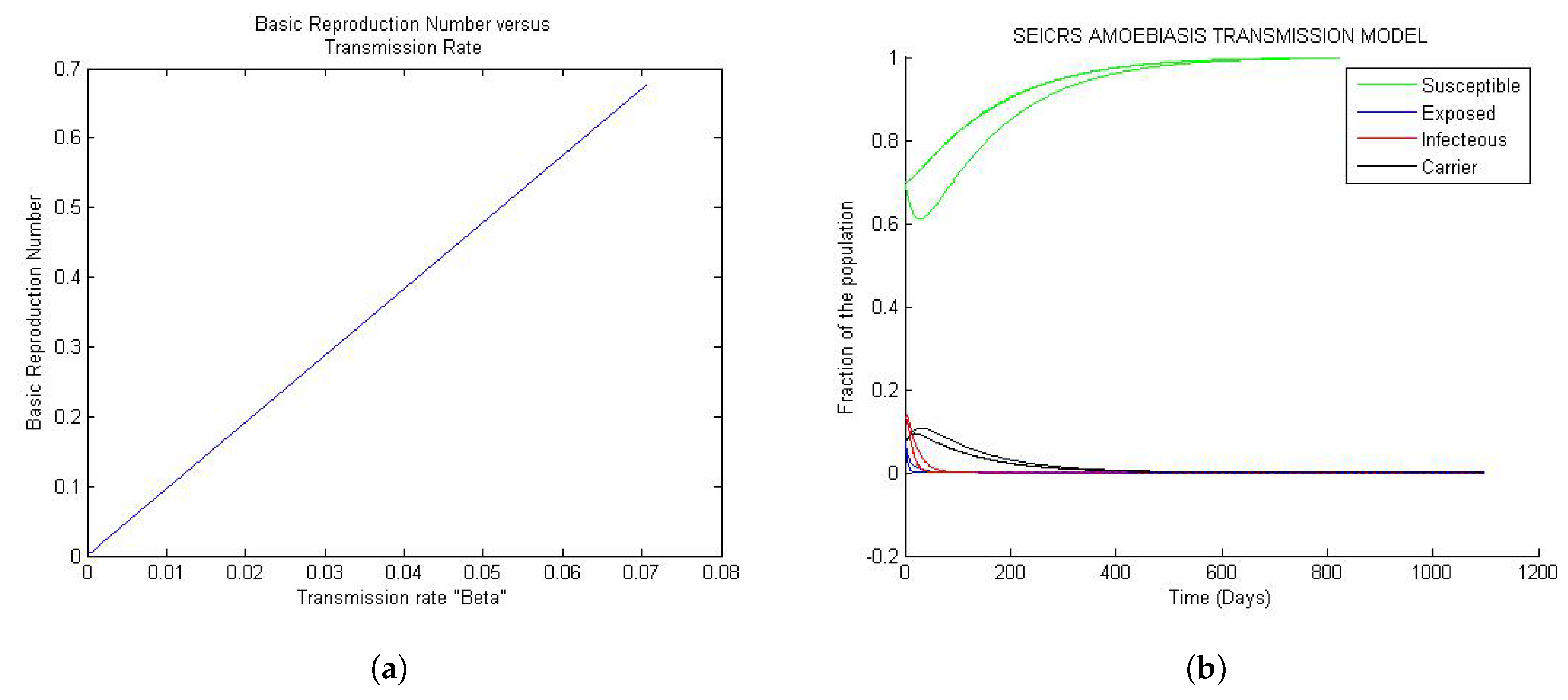
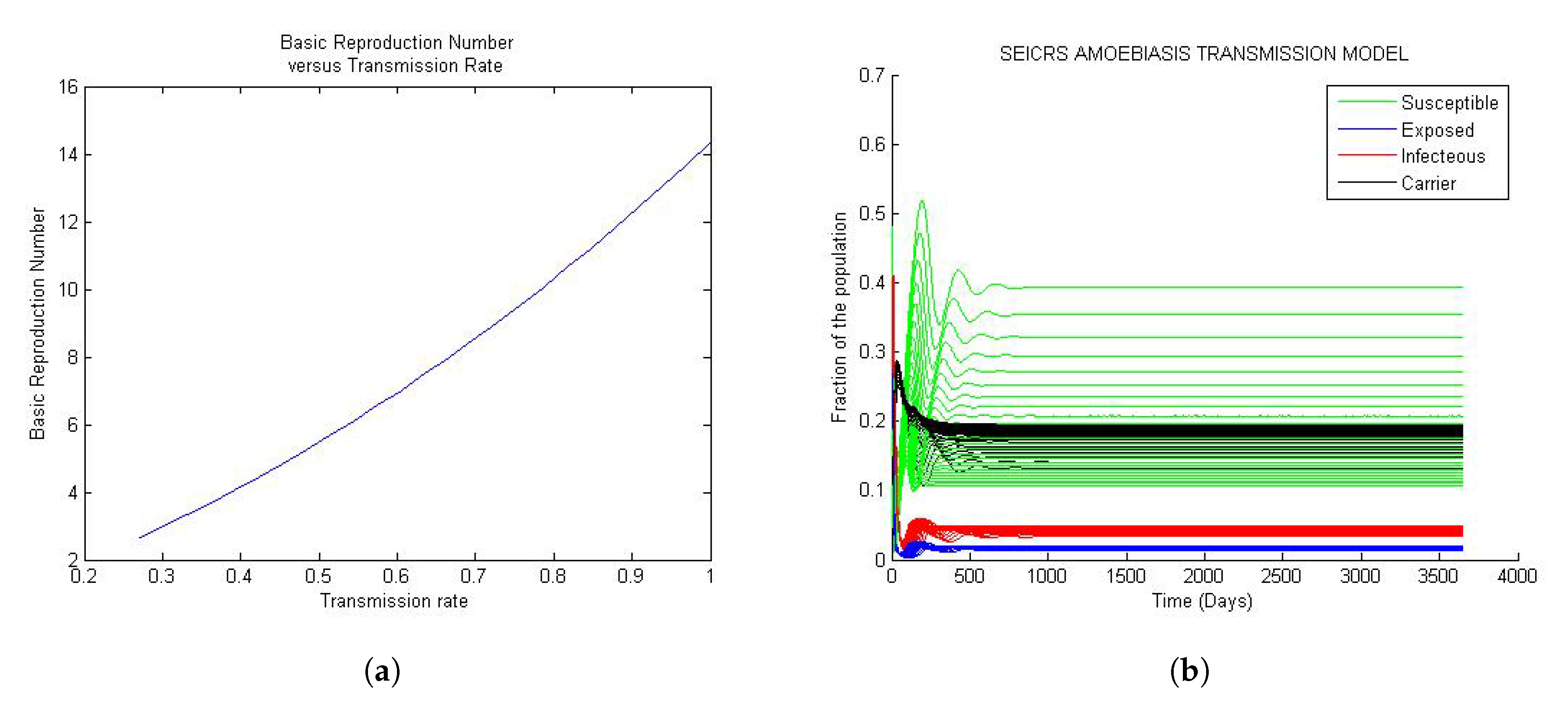
Figure 1a, Figure 2a and Figure 3a depict the change in basic reproduction number in small increments concordant with the changes in transmission rate. A pile of solution curves seen in Figure 1b, Figure 2b and Figure 3b results from 25 times (arbitrary number of times) changes (very small) in the value of every model parameter. As a result, we realize that every change in value of the parameters, however small, yields a new solution curve starting from the same initial value. Furthermore, twenty five solution curves for each of the five compartments resulting from this simulation method are more tightened for the value of the basic reproduction number less than one. Yet, they progressively lose their tightness for the value of the basic reproduction number greater than one. This phenomenon is closely related to the stability of the two steady states. To reproduce the Figure 1, Figure 2 and Figure 3 and the Figure 4, the reader would refer to Appendix A.1 and Appendix A.2 respectively.
4.1.1. Case 1:
Figure 1 represent the global trend of the model when the basic reproduction number is less than one but very small of order . If the solution is disturbed by a small perturbation from DFE state, it will definitely turn back smoothly to the initial steady state whenever the basic reproduction number is less than unit. This confirms the uniqueness of DFE = independent of the parameters for every solution curve of the model.
Looking at Figure 1a, the basic reproduction number turns out to be an increasing positive function of the transmission rate , and by Figure 1b, the 25 solution curves are tightly squeezed in one unique curve for each epidemiological class. Moreover, the model exposes a general evolution in the sizes of the S, E, I, C and R classes toward the disease-free equilibrium (DFE) approximately after 500 days since onset of the disease. The implication of the observed “tightness” suggests that, for very small values of less than one, any change in the parameters, however small, will never impact the solution of the model.
4.1.2. Case 2: Values of
The Figure 2a shows that the basic reproduction number seems to be a linear function of the transmission rate. This is expected as the initial assumption is made in order to assume different values of the parameters in the model. Likewise as in Case 1, all solution curves on the Figure 2b, converge to DFE after 500 days of the course of Amoebiasis. This demonstrates that 25 solution curves are partially tightened rendering our model moderately sensitive to the changes in the variables.
4.1.3. Case 3: Values of
Figure 3 represent the global trend of the model when the basic reproduction number is greater than unit. If the basic reproduction number is greater than unit, a small perturbation of the solution from the disease equilibrium state will never allow the return to the initial equilibrium state; the solution will rather move away from DFE to settle down at the endemic equilibrium state. Every solution settles down at its endemic equilibrium state. That is, the endemic equilibrium state of the model is unique, and it depends essentially on the parameters.
In Figure 3a, the basic reproduction is observed to be an increasing function of the transmission rate; similar to Case 1 and from Figure 3b, we observe that every solution settles down at its endemic equilibrium state. That is, the endemic equilibrium state of the model is unique, and it depends essentially on the parameters.
According to the epidemiological characteristics of amoebiasis, for the overall number of infected people, 90% of them are carriers of Entamoeba histolytica (hold cysts), and they are spending a long period of time in this state. This explains the saturation of the compartment of carrier. The remaining 10% of people are in the acute infection stage and remain in this state for a short period of time. Furthermore, given the short periods of time people stay in the E, I and R compartments, the rates associated with these periods are very high. For this reason, people leave these compartments very quickly. This explains the high fraction of people in the compartments S and C. See the Figure 3b.
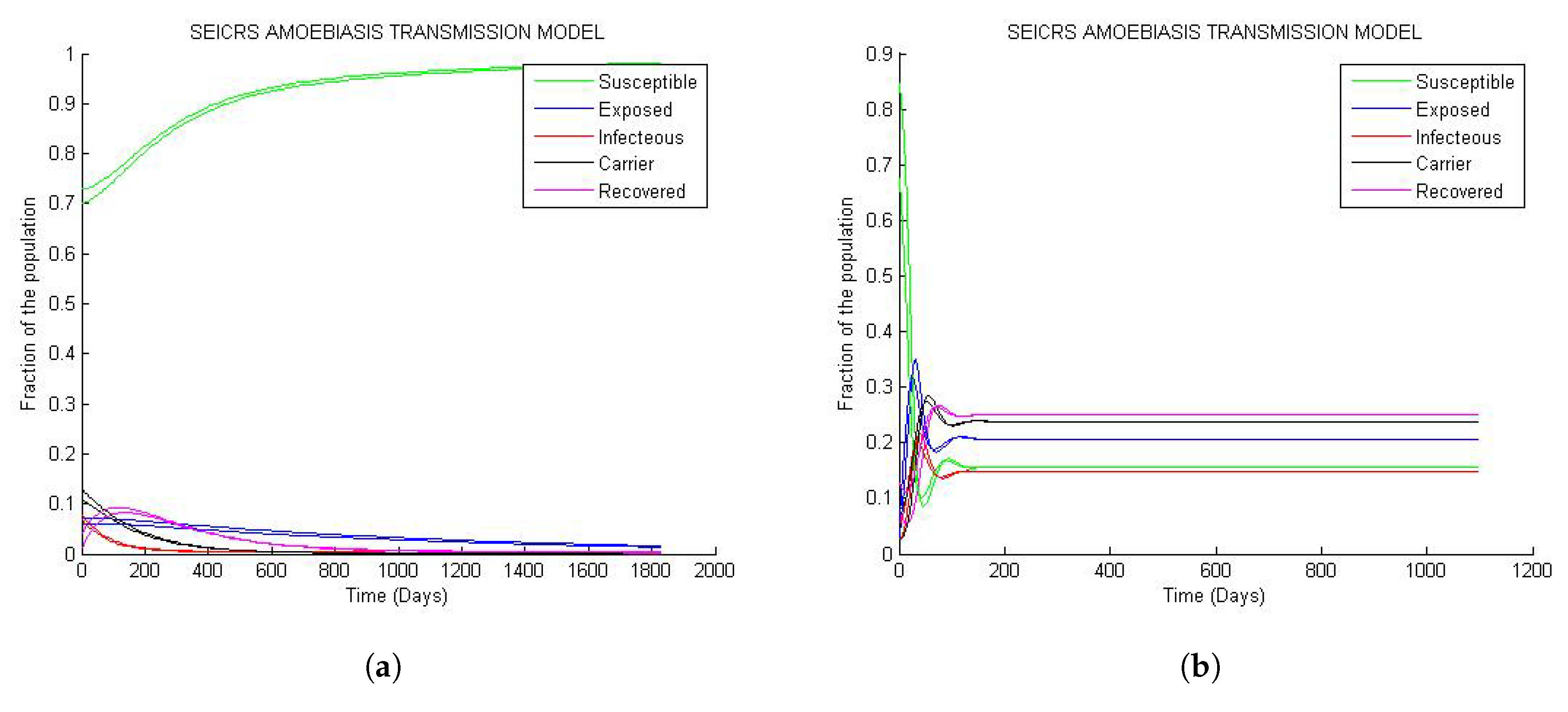
4.2. Stability of the Steady States
From Figure 4, it is clear that if two solution curves start very close to each other in the neighborhood of steady state (disease free equilibrium or endemic equilibrium), they will at a subsequent time remain close while they are converging toward the steady state. Hence, the result of Theorems 4 and 5 matchs the numerical outcome represented by the curve behavior of Figure 4a and Figure 4b respectively.
However on Figure 4b, the solution curves display oscillatory behavior around their initial values with decaying amplitudes as they are approaching their endemic steady states. This implies that the model predicts sensitive changes in fractions of the epidemiological classes near the initial values.
4.3. Sensitivity of the Basic Reproduction Number
Remarkably enough, Table 2 provides the sensitivity indices of to some approximate values of the parameters of the model. We notice, apart from , whose index is constant, changes initiated in the , , , and values have high impact on the global change in the value of the basic reproduction number . However, small changes in contribute negligibly to the changes in basic reproduction number. Suppose for each of the parameters, we allow a relative change of 4% (deceasing or increasing). According to Equation (47), the relative changes in (decreasing or increasing) resulting from the individual relative changes in these respective five parameters are 4% (for ), 3.56% (), 3.56% (for ), 0.05% (for ), −0.43% (for ), −3.31% (for ) and −3.32% (for ), respectively.
5. Discussion and Concluding Remarks
Amoebiasis is easily transferable from hand to mouth because of easy and rapid transmission. This requires rapid extinction of the susceptible population. This may be accomplished if remedial action to limit the diffusion of cysts is undertaken. As Amoebiasis becomes persistent and endemic within the population endowed with a high basic reproduction number, the fraction of susceptible individuals will drastically deplete and may even reduce to zero if the basic reproduction number is very high ( for ). This implies infected and carrier states shall dominate, and the class of the carrier population becomes prevalent. Consequentially, the spread of Amoebiasis assumes epidemic proportions. Applying the result of the sensitivity of the basic reproduction number to and , the persistent situation of the carrier class can be mitigated by shortening and (the duration of an individual in the carrier or acute infectious class, respectively). Any solution to address the issue of persistence would proceed by the reversion of the endemic disease steady state to DFE, malleable for eradication of Amoebiasis. The reversion is performed by initiating any possible measure generating a cutoff in the variation of the basic reproduction number. Some of these measures may include massive sensitization of the population for laboratory tests and preventive medication.
The application of rigorous measures (hygienic or clinical) to prevent and eradicate Amoebiasis will impact the increase in the value of the direct transmission rate red( is defined as a product of contact rates and transmission probability [26], p. 17) , transmission reducing factor and , the rate at which an acute infectious member leaves its state. We would like to highlight two events that might take place while the values of these two parameters diminish:
- The basic reproduction number is found to be remarkably sensitive to the parameters described above. Consequently, hygienic measures destabilize and decrease the direct transmission rate, as well as the transmission factor. In turn, the combined effects have a considerable contribution toward “cutting off” the basic reproduction number. This action leads to the eradication of Amoebiasis.
- The clinical measure causes the depletion rate of acute infectious state to spike. Eventually, this class/state will cease to exist due to hygienic measures as explained earlier. However, there may still be a portion of the population of carriers of cysts that can trigger Amoebiasis in future.
The proposed mathematical model for the dynamics of Amoebiasis transmission would have an additional compartment, C, for invasive Amoebiasis (SEICR epidemic model). For all practical reasons, this compartment has been considered as a key member in the case of symptomatic Amoebiasis or the acute infectious state. Absence of this component (C) takes us back to the standard models used to describe Amoebiasis. The reasons why these models may not be adequate are listed below:
- Using SEIRS epidemic model the duration of the course of Amoebiasis is made to run over a short time, i.e., the mean time an individual stays in the infectious state is reduced to . The mean duration of the carrier state, , notwithstanding its significance toward sensitivity of , is ignored.
- The SEIRS epidemic model is incapable of predicting the evolution in the carrier state, thereby ignoring a truly relevant aspect in the study of the dynamics of amoebic invasion. The model fails to accommodate the fact that the carrier state is the causative step for the development of the amoebic invasion.
- By comparison of the values of the basic reproduction number for both SEIRS epidemic model and SEICRS epidemic model given by Equation (17), it is observed that SEIRS epidemic model predicts retardant onset of Amoebiasis compared to the prediction made by SEICRS epidemic model. However, the two models will approximately have equal basic reproduction numbers for small values of ϵ and ρ.
The difference between these two basic reproduction numbers pertaining to the two paradigms has a non-negligible impact on the general dynamics trends of the two models, including the steady states, stability and sensitivity analysis. The sensitivity analysis of the basic reproduction number for the rate of transfer, , from susceptible to the exposed epidemiological classes reveals that its index value is negligibly small. This motivates us to ponder the existence of another form of epidemic model for the dynamics of Amoebiasis transmission. The new model will have the exposed class exempt from the entire system even though it might exist as a part of the general form of the SEICRS epidemic model. The authors suggest an SEICRS epidemic model based on delay differential equations.
The addition of compartments to the existing model (C in our case) enhanced the complexity of the set of equations exponentially. This defies intuitive understanding. However, more often than not, mathematical models do not obey common perception. In this case, the addition of C transformed the dynamics of the epidemic SIR epidemic modelfamily of models in such a way that an analytical solution was no longer possible!We stress that C is not a trivial addition to the existing models. Rather, it helps define amoebiasis succinctly, and the consequent qualitative analysis became imperative. This is a major contribution to capture the fine-grained nature of the model.
Another significant contribution of the manuscript is the application of forward sensitivity analysis and understanding its implications. The method led us to observe the phenomenon of the tightening of solution curves. In other words, this phenomenon is closely related to the stability of the two steady states. If the solution is disturbed by a small perturbation from the disease-free equilibrium state, it will definitely turn back smoothly to its steady state whenever the basic reproduction number is less than one. This confirms the uniqueness of DFE , independent of the parameters for every solution curve of the model. In contrast, if the basic reproduction number is greater than one, a small perturbation of the solution from the disease equilibrium state will never allow return to this equilibrium state; the solution will rather move away from DFE to settle down at the endemic equilibrium state. Every solution settles down at its endemic equilibrium state. That is, the endemic equilibrium state of the model is unique and it depends essentially on the parameters.
The comprehensive analytical and numerical study developed for Amoebiasis mathematical transmission model has created a host of reliable results that help us understand the transmission of Amoebiasis through the population. The authors concluded about key parameters for the transmission of Amoebiasis and the probable consequences resulting from any modification. As far as we can state, this study would serve as a guideline for predicting, preventing and managing the onset of Amoebiasis. SI and SIR epidemic models are efficient as those models could compute the rate of infection propagation in epidemic diseases analytically or estimate the parameters by numerical simulation. However, the model proposed by us, although more fine-grained to support additional constraints, is actually extremely intricate (because of the fine-grained analysis) with many coefficients, which makes it impossible to carry out quantitative analysis (to determine the rate of change of infection or other states). Given this problem, we proposed theorems and presented rigorous mathematical proofs establishing the qualitative relationship between the compartments of the proposed model. We interpret the outcome in terms of stability analysis and conclude that infection propagation needs to attain steady state such that the the extent and depth of infection could be evaluated in a reasonable manner. Unlike the previous models cited in the manuscript, the stability conditions present significantly greater complexity. This analysis is, therefore, both imperative for and fundamental to the disease propagation and evaluation. We believe this is a cornerstone of our approach.
Author Contributions
The authors contributed in the order their names are written in the authorship’s heading of this paper.
Conflicts of Interest
The authors declare no conflict of interest.
Appendix A
The algorithms implemented using MATLAB R2011b(7.13.0.564) depict different scenarios related to the dynamics of amoebiasis. To be precise, the algorithms below describe the three cases.
Appendix A.1. Algorithm to Generate Figure 1, Figure 2 and Figure 3
function drawing1(S0, C0, I0, E0, bet, eps, ro, gam, wa, taw, sigma, mu, maxtime); %Input parameters and initial conditions of the model
input eps, ro,gam, wa, taw, sigma, mu, maxtime.
// transmission rate, transmission reducing factor, probability of infected to carrier, recovery rate, the rate of transition from susceptible to exposed classes, the rate at which immune class decays,the rate from carrier to removed class, the natural birth rate or death rate, the interval [0 a] of integration of the model//
input %initial conditions
global a % Valid entry of the initial values
% Evaluate the possible range of the transmission beta (B) in the ranges of variation of other parameters from which beta is depending on.
% B = (k1k2k3)/[g(k3 + p)]
% g in [0.0338, 0.476], k1 in [0.0339, 0.4761], k2 in [0.0715, 0.1430]
% k3 in [6.0274 , 9.8173 ] and p in [0, 1].
//Choice of the different cases//
% Basic Reproduction Number ==
% Case 1: range of the transmission (beta) values that make
% Case 2: range of the transmission (beta) values that make
% Case 3: range of the transmission (beta) values that make
The Graphics component:
Case 1: Minimum Transmission
Case 2: Transmit
Case 3: Max Transmission
== the initial susceptible value; == initial carrier value; == the initial infected value; == initial exposed value;
if
Return Invalid;
end
% Integration of the function f(t,x), The solution to amoebiasis transmission.
% Main Iterative numerical method
tspan = maxtime;
= [];
B = zeros(1,var2);
for j = 1:var2
a(1) = beta(j);
= a(1)×sigma×((taw+mu) + epslon(j)×rho(j)×gam)
/((sigma + mu)×(gam + mu)×(taw + mu));
B(1,j) = ;
= ode45(’diffamoeba’,tspan,); %Runge-Kutta 4th and 5th order mixed
S = x(:,1);E = x(:,2);I = x(:,3);C = x(:,4);
plot(t,S,’g’,t,E,’b’,t,I,’r’,t,C,’k’)
plot(beta,B)
end
Appendix A.2. Algorithm to Generate Figure 4
function amoebiasis(, , , , bet, eps, ro, gam, wa, taw, sigma, mu, maxtime);
% Input of the initial conditions and the parameters of the model
input eps, ro,gam, wa, taw,sigma, mu, maxtime
//transmission rate, transmission reducing factor, probability of infected to carrier, recovery rate, the rate of transition from susceptible to exposed classes, the rate at which immune class decays,the rate from carrier to removed class, the natural birth rate or death rate, the interval [0 a] of integration of the model//
input initial conditions
% To evaluate the reproduction number R0
* Analysis of the basic reproduction number and its implication **
* Stability of the steady state solutions **
= bet×sigma((taw + mu) + eps×ro×gam)
/((sigma + mu)×(gam + mu)×(taw + mu));** Calculation of the basic reproduction number **
if
% Determination of the endemic disease equilibrium point
D = (a(5) + a(6) + a(8)) (a(4) + a(8))/a(5) + a(6)
(1 + a(3)a(4))/(a(7) + a(8)));
Ieq = (a(6) + a(8))/D×(1−1/); ** Size of Infectious class **
Eeq = (a(4) + a(8))/a(5)×Ieq; ** Size of exposed class **
Ceq = a(3)×a(4)×Ieq/(a(7) + a(8)); ** Size of carrier class **
Seq = 1/; ** Size of susceptible class **
A = [Seq Eeq Ieq Ceq];
Mini = min(A); %The lower bound of stability for endemic steady state.
else
Seq = 1;
Ieq = 0;
Eeq = (a(4) + a(8))/a(5)×Ieq;
Ceq = a(3)×a(4)×Ieq/(a(7) + a(8));
end
% Valid entry of the initial values
// //
if
Display ‘ Invalid, Restart. ’
end
% Integration of the function f(t,x); the solution to the amoebiasis transmission; main iterative numerical method
tspan = maxtime; ** Period of study **
= []; ** Initial sizes **
options = odeset(’RelTol’,1e-6); ** Error bound **
= ode45(’diffamoeba’,tspan,x0,options);
S = x(:,1); E = x(:,2); I = x(:,3); C = x(:,4);
;
Plot;
end
%Print the steady state components%
////
Appendix A.3. Algorithm of Sub-Function “diffamoeba()”
function y = diffamoeba(t,x)
% y is a column matrix whose component are variations in
% a is a raw matrix of coefficients a(1) = bet, a(2) = eps, a(3) = ro, a(4) = gam, a(5) = sigma,
% a(6) = wa, a(7) = taw and a(8) = mu.
% x is a raw matrix of the variables
** Susceptible, exposed, infectious and carrier sizes are components of the vector x. **
global a; ** Declaration of the matrix of coefficients as global variable **
y=zeros(size(x)); ** Initialization of y as zero vector. **
* The next is the evaluation of the function f(t,x) **
y(1,1) = (a(8) + a(6))−(a(1)×x(3) + a(2)×a(1)×x(4) + (a(8) + a(6)))×
x(1)−a(6)×(x(2) + x(3) + x(4));
y(2,1) = (a(1)×x(3) + a(2)×a(1)×x(4))×x(1)−(a(5) + a(8))×x(2);
y(3,1) = a(5)×x(2)−(a(4) + a(8))×x(3);
y(4,1) = a(3)×a(4)×x(3)−(a(6) + a(8))×x(4);
end
References
- Hotez, P.J.; Molyneux, D.H.; Fenwick, A.; Kumaresan, J.; Sachs, S.E.; Sachs, J.D.; Savioli, L. Control of neglected tropical diseases. N. Engl. J. Med. 2007, 357, 1018–1027. [Google Scholar] [CrossRef] [PubMed]
- Stauffer, W.; Abd-Alla, M.; Ravdin, J.I. Prevalence and Incidence of Entamoeba histolytica Infection in South Africa and Egypt. Arch. Med. Res. 2006, 37, 265–268. [Google Scholar] [CrossRef] [PubMed]
- Walsh, J.A. Problems in Recognition and Diagnosis of Amebiasis: Estimation of the Global Magnitude of Morbidity and Mortality. Rev. Infect. Dis. 1986, 8, 228–238. [Google Scholar] [CrossRef] [PubMed]
- Prevalence and Incidence of amoebiasis. Available online: http://www.rightdiagnosis.com/a/amebiasis/prevalence.htm (accessed on 20 July 2017).
- Hertz, R.; Lulu, S.B.; Shahi, P.; Trebicz, W.; Benhar, M.; Ankri, S. Proteomic Identification of S-Nitrosylated Proteins in Parasite Entamoeba histolytica by Resin-Assisted Capture: Insights into the Regulation of the Gal/GalNAC Lectin by Nitric Oxide. PLoS ONE 2014, 9, e91518. [Google Scholar] [CrossRef] [PubMed]
- Thibeaux, R.; Weber, C.; Hon, C.C.; Dillie, M.A.; Avé, P.; Coppée, J.-Y.; Labruyère, E.; Guillén, N. Identification of the Virulence Landscape Essential for Entamoeba histolytica Invasion of the Human Colon. PLoS Pathog. 2013, 9, e1003824. [Google Scholar] [CrossRef] [PubMed]
- Haque, R.; Ali, I.K.M.; Petri, W.A., Jr. Prevalence and immune response of Entamoeba histolytica infection in preschool children in Bangladesh. Am. J. Trop. Med. Hyg. 1999, 60, 1031–1034. [Google Scholar] [CrossRef] [PubMed]
- Jackson, T.F.; Gathira, V.; Simjee, A.E. Seroepidemiological Study of antibody responses to the zymodemes of Entamoeba histolytica. Lancet 1985, 325, 716–719. [Google Scholar] [CrossRef]
- Xeménez, C.; Moran, P.; Rajas, L.; Valadez, A.; Gomez, A. Reassessment of the epidemiology of amebiasis: State of the arth. Infect. Genet. Evol. 2009, 9, 1023–1032. [Google Scholar] [CrossRef] [PubMed]
- Petri, W.A., Jr.; Singh, U. Diagnosis and Management of Amebiasis. Clin. Infect. Dis. 1999, 29, 1117–1125. [Google Scholar] [CrossRef] [PubMed]
- Samie, A.; ElBakri, A.; AbuOdeh, R. Amoebiasis in the Tropics: Epidemiology and Pathogenesis. In Current Topics in Tropical Medicine; InTech: Rijeka, Croatia, 2012. [Google Scholar]
- Dhawan, V.K.; Cleveland, K.O.; Cantey, J.R. Amoebiasis. Available online: http://emedicine.medscape.com/article/212029-overview (accessed on 20 February 2017).
- Caballero-Salcedo, A.; Viveros-Rogel, M.; Salvatierra, B.; Tapia-Conyer, R.; Sepulveda-Amor, J.; Gutierrez, G.; Ortiz-Ortiz, L. Seroepidemiology of amebiasis in Mexico. Am. J. Trop. Med. Hyg. 1994, 50, 412–419. [Google Scholar] [CrossRef] [PubMed]
- Lawson, L.L.O.; Bailey, J.W.; Beeching, N.J.; Gurgel, R.G.; Cuevas, L.E. The stool examination reports amoeba cysts: Should you treat in the face of over diagnosis and lack of specificity of light microscopy? Trop. Doctor 2004, 34, 28–30. [Google Scholar] [CrossRef] [PubMed]
- Tanyuksel, M.; Petri, W.A., Jr. Laboratory Diagnosis of Amebiasis. Clin. Microbiol. Rev. 2003, 16, 713–729. [Google Scholar] [CrossRef] [PubMed]
- Stanley, S.L., Jr. Protective Immunity to Amebiasis: New Insights and New Challenges. J. Infect. Dis. 2001, 184, 504–606. [Google Scholar] [CrossRef] [PubMed]
- Hategekimana, F.; Saha, S.; Chaturvedi, A. Amoebiasis Transmission and Life cycle: A continuous state description by virtue of existence and uniqueness. Glob. J. Pure Appl. Math. 2016, 12, 375–390. [Google Scholar]
- Wang, Y.; Jin, Z.; Yang, Z.; Zhang, Z.-K.; Zhou, T.; Sun, G.-Q. Global analysis of an SIS model with an infective vector on complex network. Nonlinear Anal. Real World Appl. 2012, 13, 543–557. [Google Scholar] [CrossRef]
- Anderson, R.M.; May, R.M. Population biology of infectious disease I. Nature 1979, 180, 316–367. [Google Scholar] [CrossRef]
- Hethcote, H.W. The Mathematics of Infectious diseases. SIAM Rev. 2000, 42, 599–653. [Google Scholar] [CrossRef]
- Gao, L.Q.; Hethcote, H.W. Disease transmission models with density-dependent demographics. J. Math. Biol. 1992, 30, 717–731. [Google Scholar] [CrossRef] [PubMed]
- Clumax, M. Speciality Consultation Service. Available online: http://www.medall.in/health-information/disease/infectious-disease/amoebiasis/ (accessed on 16 June 2017).
- Logemann, H.; Ryan, E.P. Ordinary Differential Equation, Analysis, Qualitative Theory and Control; Springer: London, UK, 2014. [Google Scholar]
- Wiggis, S. Texts In Applied Mathematics: Introduction to Applied Nonlinear Dynamical Systems and Chaos; Springer Science and Business Media: New York, NY, UA, 2003; Volume 2. [Google Scholar]
- Diekmann, O.; Heesterbeek, J.A.P.; Metz, J.A.J. On the definition and the computation of the basic reproduction ratio in models for infectious diseases in heterogeneous population. J. Math. Biol. 1990, 28, 365–382. [Google Scholar] [CrossRef] [PubMed]
- Keeling, M.J.; Pejna, R. Modeling Infectious Diseases in Humans and Animals; Princeton University Press: Princeton, NY, USA, 2008. [Google Scholar]
- Driessche, P.; Watmough, J. Reproduction numbers and sub-threshold endemic equilibria for compartmental models of disease transmission. Math. Biosci. 2002, 180, 29–48. [Google Scholar] [CrossRef]
- Otieno, G.; Koske, J.K.; Mutiso, J.M. Cost Effectiveness Analysis of Optimal Malaria Control Strategies in Kenya. Mathematics 2016, 4, 14. [Google Scholar] [CrossRef]
- Coddington, A.E.; Levinson, N. Theory of Ordinary Differential Equations; Tata McGraw-Hill: New Dheli, India, 2010. [Google Scholar]
- Perko, L. Differential Equation and Dynamical Systems, 3rd ed.; Springer-Verlag: New York, NY, USA, 2014. [Google Scholar]
- Murray, J.D. Mathematical Biology: I. An Introduction, 3rd ed.; Springer: London, UK, 2002. [Google Scholar]
- Trawicki, M.B. Deterministic Seirs Epidemic Model for Modeling Vital Dynamics, Vaccinations, and Temporary Immunity. Mathematics 2017, 5, 7. [Google Scholar] [CrossRef]
- Kamgang, J.C.; Sallet, G. Computation of threshold conditions for epidemiological models and global stability of the disease-free equilibrium (DFE). Math. Biosci. 2008, 213, 1–12. [Google Scholar] [CrossRef] [PubMed]
- Xiaolin, F.; Wang, L.; Teng, Z. Global dynamics for class of discrete SEIRS epidemic models with general nonlinear incidence. Adv. Differ. Eq. 2016, 2016, 123. [Google Scholar]
- Cooke, K.L.; van den Driessche, P. Analysis of an SEIRS epidemic model with two delays. J. Math. Biol. 1996, 35, 240–260. [Google Scholar] [CrossRef] [PubMed]
- Agrawal, A. Global analysis of an SEIRS epidemic model with new modulated saturated incidence. Commun. Math. Biol. Neurosci. 2014, 2014, 1–11. [Google Scholar]
- Nkamba, L.N.; Ntaganda, J.M.; Abboubakar, H.; Kamgang, J.C.; Lorenzo, C. Global stability of a SVEIR epidemic model: Application to poliomyelitis transmission dynamics. Open J. Model. Simul. 2017, 5, 98–112. [Google Scholar] [CrossRef]
- Chitnis, N.; Cushing, J.; Hyman, J. Bifurcation analysis of a mathematical model for malaria transmission. SIAM J. Appl. Math. 2006, 67, 24–45. [Google Scholar] [CrossRef]
- Abd-Alla, M.D.; Jackson, T.F.; Rogers, T.; Reddy, S.; Ravdin, J.I. Mucosal immunity to asymptomatic Entamoeba histolytica and Entamoeba dispar infection is associated with a peak intestinal anti-lectin immunoglobulin A antibody response. Infect. Immun. 2006, 74, 3897–3903. [Google Scholar] [CrossRef] [PubMed]
- Amebiasis: Overview, Causes and Symptoms. Available online: http://www.healthline.com/health/amebiasis (accessed on 23 June 2017).
Figure 1.
General trends of the model for values of small than one: (a) Curve of the versus ; (b) 25 solution curves’ behavior.
Figure 1.
General trends of the model for values of small than one: (a) Curve of the versus ; (b) 25 solution curves’ behavior.
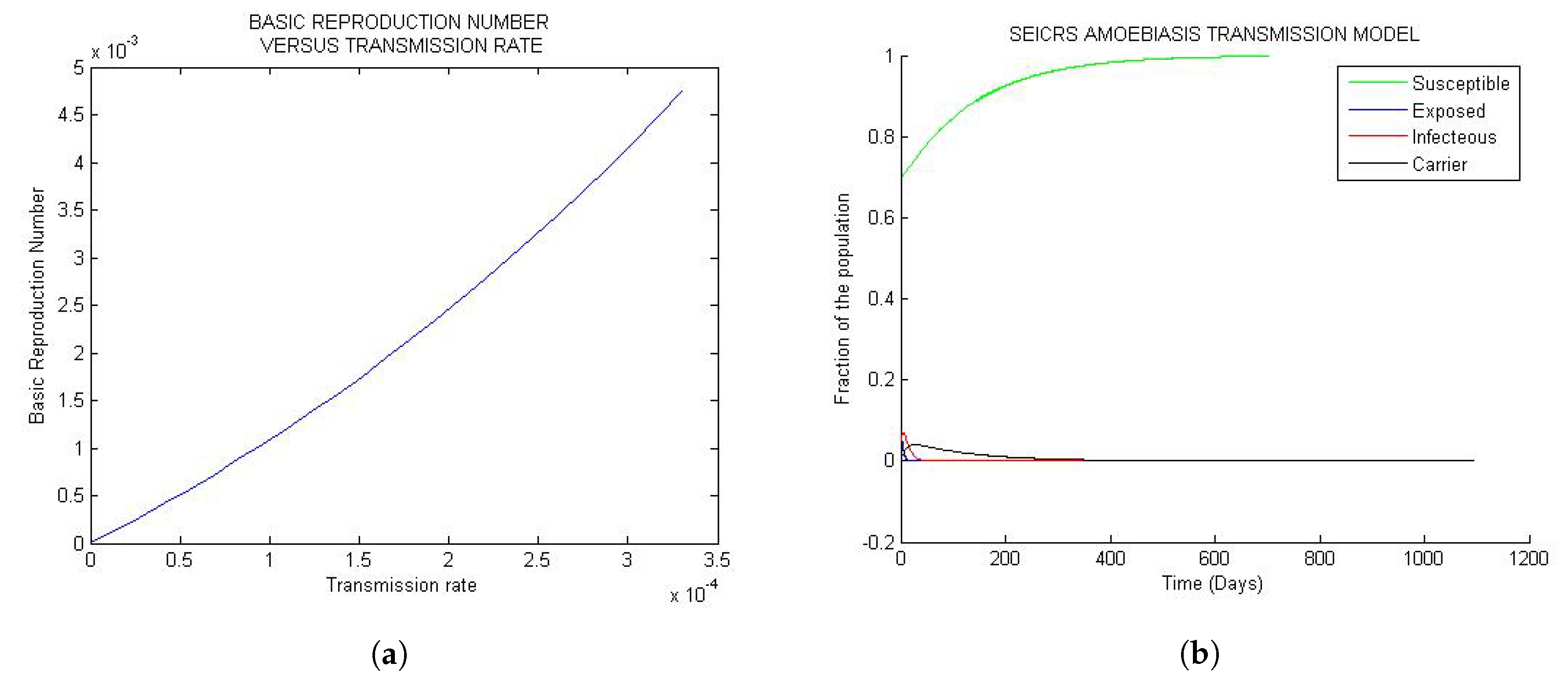
Figure 2.
General trend of the model for values of very close to one: (a) Curve of the versus ; (b) structure of the 25 solutions-curve.
Figure 2.
General trend of the model for values of very close to one: (a) Curve of the versus ; (b) structure of the 25 solutions-curve.

Figure 3.
General trend of the model when is greater than one: (a) Curve of the versus ; (b) 25 solution curves of the model.
Figure 3.
General trend of the model when is greater than one: (a) Curve of the versus ; (b) 25 solution curves of the model.

Figure 4.
Asymptotic stability of the steady states: (a) Asymptotic stability of DFE; (b) asymptotic stability of the endemic equilibrium.
Figure 4.
Asymptotic stability of the steady states: (a) Asymptotic stability of DFE; (b) asymptotic stability of the endemic equilibrium.


Table 1.
Table of parameters.
| Symbol | Description | Unit |
|---|---|---|
| Force of infection | ||
| Direct transmission rate | ||
| Transmission reducing factor | Dimensionless | |
| Average latency period | ||
| Average infectious period of acute infectiousness. | ||
| Average temporary immune period | ||
| Average infectious period of carrier | ||
| Population’s crude birth (per capita death) rate | ||
| Probability of an infectious to becomes carrier | Dimensionless |
Table 2.
Range of model parameters and sensitivity index of .
| Parameter | Unit | Range | Baseline | Sensitivity Index of |
|---|---|---|---|---|
| (time) | 0.6 | 1 | ||
| Dimensionless | 0.084 | 0.8905 | ||
| Dimensionless | 0.95 | 0.8905 | ||
| (time) | 6.8493 | −0.8307 | ||
| (time) | 0.1 | −0.1089 | ||
| (time) | 0.0714 | 0.0134 | ||
| (time) | −0.8283 | |||
| (time) | 0.0588 | — |
© 2017 by the authors. Licensee MDPI, Basel, Switzerland. This article is an open access article distributed under the terms and conditions of the Creative Commons Attribution (CC BY) license (http://creativecommons.org/licenses/by/4.0/).
Share and Cite
MDPI and ACS Style
Hategekimana, F.; Saha, S.; Chaturvedi, A. Dynamics of Amoebiasis Transmission: Stability and Sensitivity Analysis. Mathematics 2017, 5, 58. https://doi.org/10.3390/math5040058
AMA Style
Hategekimana F, Saha S, Chaturvedi A. Dynamics of Amoebiasis Transmission: Stability and Sensitivity Analysis. Mathematics. 2017; 5(4):58. https://doi.org/10.3390/math5040058
Chicago/Turabian StyleHategekimana, Fidele, Snehanshu Saha, and Anita Chaturvedi. 2017. "Dynamics of Amoebiasis Transmission: Stability and Sensitivity Analysis" Mathematics 5, no. 4: 58. https://doi.org/10.3390/math5040058
Note that from the first issue of 2016, this journal uses article numbers instead of page numbers. See further details here.