Extending the Characteristic Polynomial for Characterization of C20 Fullerene Congeners


1
Doctoral School of Chemistry, Babes-Bolyai University, 400028 Cluj, Romania
2
Department of Physics and Chemistry, Technical University of Cluj-Napoca, 400641 Cluj, Romania
*
Author to whom correspondence should be addressed.
Mathematics 2017, 5(4), 84; https://doi.org/10.3390/math5040084
Submission received: 28 November 2017
/
Revised: 28 November 2017
/
Accepted: 13 December 2017
/
Published: 19 December 2017
(This article belongs to the Special Issue Applied and Computational Statistics)
Abstract
:The characteristic polynomial (ChP) has found its use in the characterization of chemical compounds since Hückel’s method of molecular orbitals. In order to discriminate the atoms of different elements and different bonds, an extension of the classical definition is required. The extending characteristic polynomial (EChP) family of structural descriptors is introduced in this article. Distinguishable atoms and bonds in the context of chemical structures are considered in the creation of the family of descriptors. The extension finds its uses in problems requiring discrimination among same-patterned graph representations of molecules as well as in problems involving relations between the structure and the properties of chemical compounds. The ability of the EChP to explain two properties, namely, area and volume, is analyzed on a sample of C20 fullerene congeners. The results have shown that the EChP-selected descriptors well explain the properties.
Keywords:
characteristic polynomial (ChP); molecular descriptors; fullerene congeners; C20 fullerene; structure–property relationshipsPACS:
02.10.Ox; 02.50.Sk; 02.50.TtMSC:
05C31; 12E10; 60E10; 55R40; 47N601. Introduction
The term ‘secular function’ has been used for what is now called a characteristic polynomial (ChP, in some of the literature, the term secular function is still used). The ChP was used to calculate secular perturbations (on a time scale of a century, i.e., slow compared with annual motion) of planetary orbits [1]. The first use of the ChP (|λ∙Id−Ad|, where Id is the identity matrix, and Ad is the adjacency matrix) in relation with chemical structure appeared after the discovery of wave-based treatment at the microscopic level [2]. The Hückel’s method of molecular orbitals is actually the first extension of the ChP definition. He uses the ‘secular determinant’—the determinant of a matrix which is decomposed as |E∙Id−Ad|, standing with the energy of the system (E instead of λ)—to approximate treatment of π electron systems in organic molecules [2].
The second extension of the ChP was found by Hartree [3,4] and Fock [5,6] by going in a different direction with the approximation of the wavefunction treatment. They actually found the same older eigenvector–eigenvalue problem (§20 in [7]; T1 in [8]) in Slater’s treatment [9,10] of molecular orbitals. More generally (and older), the eigen-problem (finding of eigenvalues and eigenvectors) is involved in any Hessian [11] matrix [A] ([Ad] → [A], where Ad is the adjacency matrix). The Laplacian polynomial is a polynomial connected with the ChP (in Table 1). This uses a modified form (the Laplacian matrix, [La]) of the adjacency matrix ([Ad]), [La] = [Dg] − [Ad], where [Dg] simply counts on the main diagonal the number of the atom’s bonds (the rest of its elements are null; for convenience with the graph-theory-related concept, it was denoted [Dg], from vertex degree). The ChP is related also to the matching polynomial [12], degenerating to the same expression for forests (disjoint union of trees). Adapting [13] for molecules, a k-matching in a molecule is a matching with exactly k bonds between different atoms; see §3.1 & §3.3 in [14] for details. Each set containing a single edge is also an independent edge set; the empty set should be treated as an independent edge set with zero edges—this set is unique due to the constraint of connecting different atoms, where the matching may involve no more than [n/2] bonds, where n is the number of atoms. It is possible to count the k-matches [15], but, nevertheless, it is a hard problem [16], as well as to express the derived Z-counting polynomial [17] and matching polynomial—both are defined using m(k) as the k-matching number of the selected molecule, as shown in Table 1 (where n is the number of atoms).
A topological description of a molecule requires the storing of the bonds (as adjacencies) between the atoms and the atoms themselves (as identities). If this problem is simplified at maximum, by disregarding the atom and bond types, then the molecule is seen as an undirected and unweighted graph. The graph structure can be translated into the informational space by numbering the atoms. Unfortunately, this procedure also induces an isomorphism—the isomorphism of numbering, which may collapse into a nondeterministic polynomial time to be solved—see [18]. This is a reason for the desire of graph invariants, e.g., which do not depend on the numbering made on the graph.
Once the atoms (or the vertices) are numbered, the information can be simply stored as lists of vertices (V) and edges (E), and the graph structure of the molecule is associated with the pair G = (V, E). An equivalent representation is obtained using matrices. The adjacencies ([Ad]) are simply stored with 0 when no bond connects the atoms and 1 when a bond connecting the atoms exists. The identity matrix ([Id]) identifies the atoms by placing 1 on the main diagonal and 0 otherwise.
The ChP is the natural construction of a polynomial (in λ) in which the eigenvalues of [Ad] are the roots of the ChP as follows:
λ is an eigenvalue of [Ad] → there exists eigenvector [v] ≠ 0 such that λ∙[v] = [Ad] × [v].
As a consequence:
(λ∙[Id] − [Ad])∙[v] = 0; since [v] ≠ 0 → λ∙[Id] − [Ad] is singular → |λ∙[Id] − [Ad]| = 0.
Finally,
ChP ← |λ∙[Id] − [Ad]|.
ChP is a polynomial (in λ) of degree n, where n is the number of atoms. The ChP finds its uses in the topological theory of aromaticity [19,20], structure-resonance theory [21], quantum chemistry [22], and counts of random walks [23], as well as in eigenvector–eigenvalue problems [24].
This definition allows extensions. A natural extension is to store in the identity matrix ([Id]) non-unity instead of unity values ([Id]i,j = 1 → [Id]i,j ≠ 1) accounting for the atom types, as well as to store in the adjacency matrix ([Ad]) non-unity instead of unity values accounting for the bond types ([Ad]i,j = 1 → [Ad]i,i ≠ 1. This extension was subjected to study in the context of deriving structural descriptors useful for structure–property relationships.
2. Materials and Methods
2.1. Graphs, Matrices, and the Characteristic Polynomial
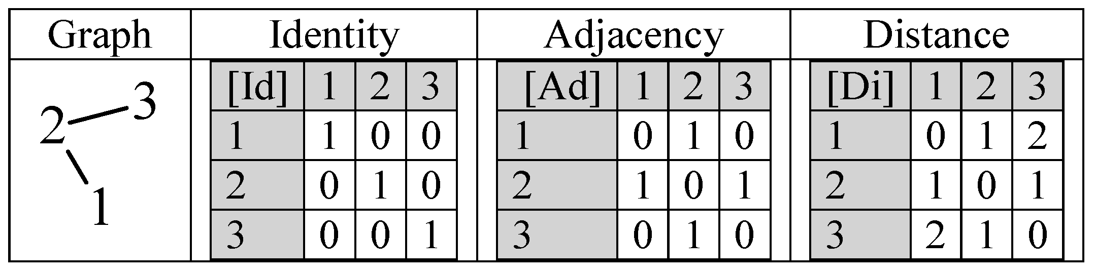
The topology of a graph structure could be expressed as matrices, and, in this regard, three of them are more frequently used: identity, adjacency (vertex–vertex, edge–edge, and vertex–edge), and distance matrices can be built (Table 2).
The matrices reflect in a 1:1 fashion the graph if the full graph is stored (each vertex pair stored twice, in both ways). The matrices of vertex adjacency ([Ad]) and of edge adjacency are square and the double enumeration of the edges is reflected in symmetry relative to the main diagonal (see Figure 1).
ChP is the natural construction of a polynomial in which the eigenvalues of the [Ad] are the roots of the ChP. ChP is a polynomial in λ of degree n, where n is the number of atoms. A natural extension is to store in [Id] (instead of unity) non-unity values accounting for the atom types, as well as to store in [Ad] (instead of unity) non-unity values accounting for the bond types.
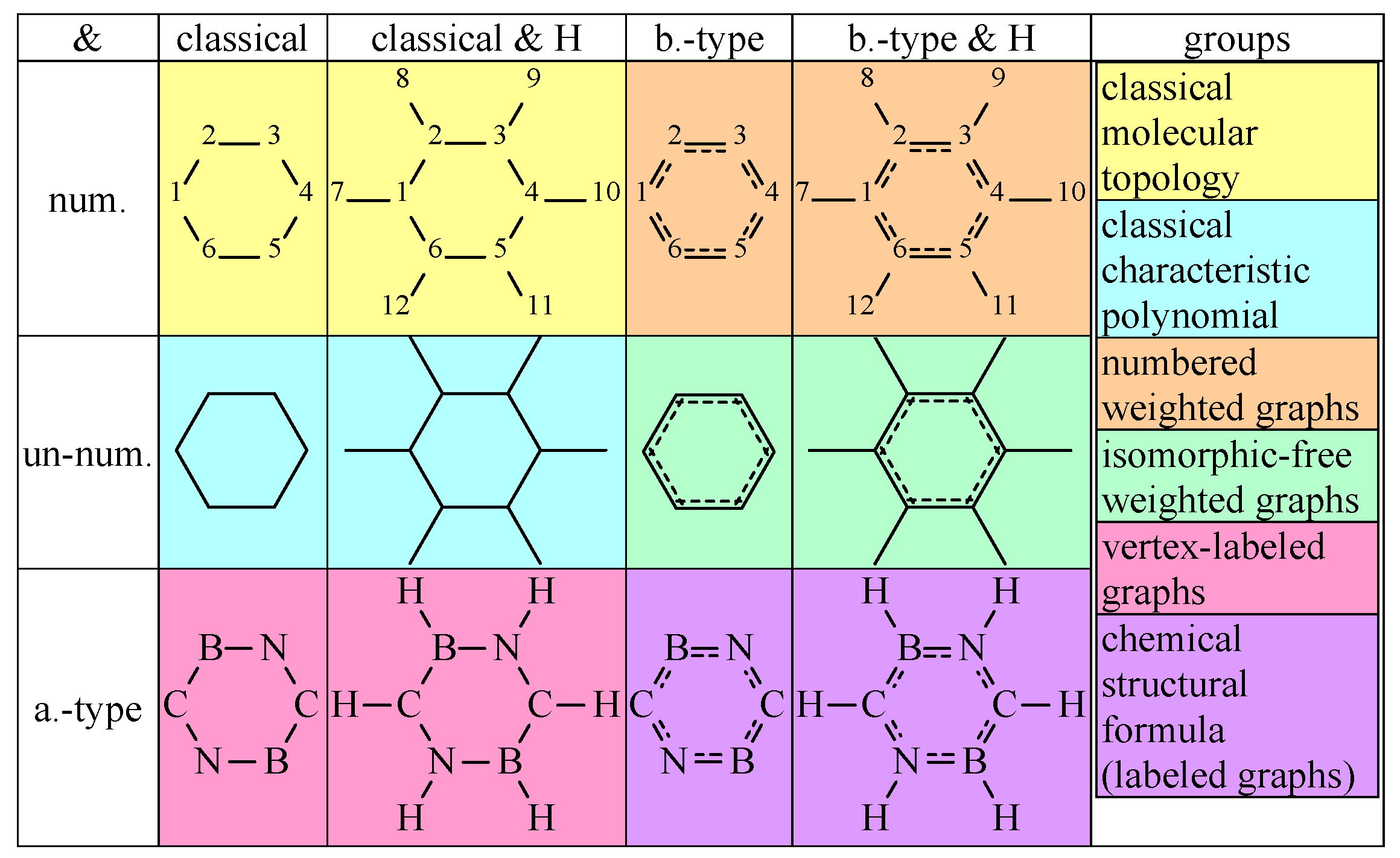
An extremely important problem in chemistry is to uniquely identify a chemical compound. If the visual identification (looking at the structure) seems simple, for compounds of large size, this alternative is no longer viable. The data related to the structure of the compounds stored into the informational space may provide the answer to this problem. Nevertheless, together with the storing of the structure of the compound another issue is raised—namely, the arbitrary numbering of the atoms (Figure 2).
For a chemical structure with N atoms stored as a (classical molecular) graph, there exist exactly N! possibilities for numbering the atoms. Unfortunately, storing the graphs as lists of edges and (eventually) vertices does not provide a direct tool to check this arbitrary differentiation due to the numbering. The same situation applies to the adjacency matrices. Therefore, seeking for graph invariants is perfectly justified: an invariant (graph invariant) does not depend on numbering. The adjacency matrix is not a graph invariant and, therefore, it is necessary to go further than the adjacencies.
Important classes of graph invariants are the graph polynomials. To this category belongs the ChP—a graph invariant encoding important properties of the graph. On the other hand, unfortunately, ChP does not represent a bijective image of the graph, as there exist different graphs with the same ChP (i.e., cospectral graphs—the smallest cospectral graphs occurs for 5 vertices [25]). In order to count the cospectral graphs, one should compare A000088 and A082104 [26,27]. The ideal situation is that the invariant should be uniquely assigned to each structure, but this kind of invariant is difficult to find. A procedure to generate a non-degenerate invariant proposed by IUPAC is the international chemical identifier (InChI), which converts the chemical structure to a table of connectivity expressed as a unique and predictable series of characters [28].
Despite this inconvenience (not representing a bijective image of the graph) due to its link with the partition of the energy [2], the ChP seems to be one of the best alternatives for quantifying the information from the chemical structure.
Previously, researchers have shown the performance of estimation and/or prediction of the ChP on nonane isomers [29,30,31] as well as in the case of carbon nanostructures [32,33]. Furthermore, an online environment has been developed to assist researchers in the calculation of polynomials based on different approaches; this includes the ChP [34].
2.2. Characteristic Polynomial Extension
When doing calculations on molecular graphs, it is important to consider that, with the increase in the simplification in the graph representation (such as neglecting the type of the atom, bond orders, geometry in the favor of topology), the degeneration of the whole pool of possible calculations increases and there are more molecules with the same representation. This is favorable for the problems seeking similarities but is clearly unfavorable for the problems seeking dissimilarities.
A necessary step to accomplish better coverage of similarity vs dissimilarity dualism is to build and use a family of molecular descriptors, large enough to be able to provide answers for all. In the natural way, such a family should possess a ‘genetic code’—namely, a series of variables from which to (re)produce a (one by one) molecular descriptor, all descriptors being therefore obtained in the same way. It is expected that all individuals of the family are independent of the numbering of the atoms in the molecule (should be molecular invariants).
The construction of such a family needs to consider the following:
- Molecules carry both topological and geometrical features (see Figure 3);
- Atom and bond types are essential factors in the expression of the measurable properties;
- Atom and/or bond numbering induces an undesired isomorphism;
- Geometry and bond types induce other kinds of isomorphism.
The representation of a molecule could be done using identity and adjacency (Figure 4).
The distinct identities from Figure 4 are given using a, b, and c as variables in the case of adjacency and using d, e, and f as variables in the case of identity. This formalism allows the introduction of a natural extension of the ChP from graphs to molecules. There is no determinism in selecting the values of a–f. However,
- If a = b = c = d = e = f = 1 then ChPE ← ChP as in classical molecular topology.
- If a = b = c = 1.5−1, then [A] accounts for the (inverse of the) bond order.
- If a = 1.35−1, b = 1.448−1, and c = 1.493−1 then [A] accounts for the (inverse of the) geometrical distance (in Å).
- If d = 12/294, e = 14/294, and f = 10.8/294, then [I] accounts for atomic mass relative to Uuo, the last element from the 7th period of the system of elements.
- If d = 2267/ρref, e = 1026/ρref, and f = 2460/ρref, then [I] accounts for the solid state relative density (in m3/kg); ρref can be fixed to 30,000.
- If d = 2.55/4.00, e = 3.04/4.00, and f = 2.04/4.00, then [I] accounts for electronegativity relative to Fluorine when the Pauling scale is used.
- If d = 1086.2/1312, e = 1402.3/1312, and f = 800.6/1312, then [I] accounts for the first potential of ionization relative to the potential of ionization for Hydrogen.
- If d = 3820/3820, e = 63/3820, and f = 2573/3820, then [I] accounts for melting point relative to the diamond allotrope of Carbon (in K).
- If d = 1/4, e = 1/4, and f = 1/4, then [I] accounts for the number of hydrogen atoms attached relative to the score of CH4.
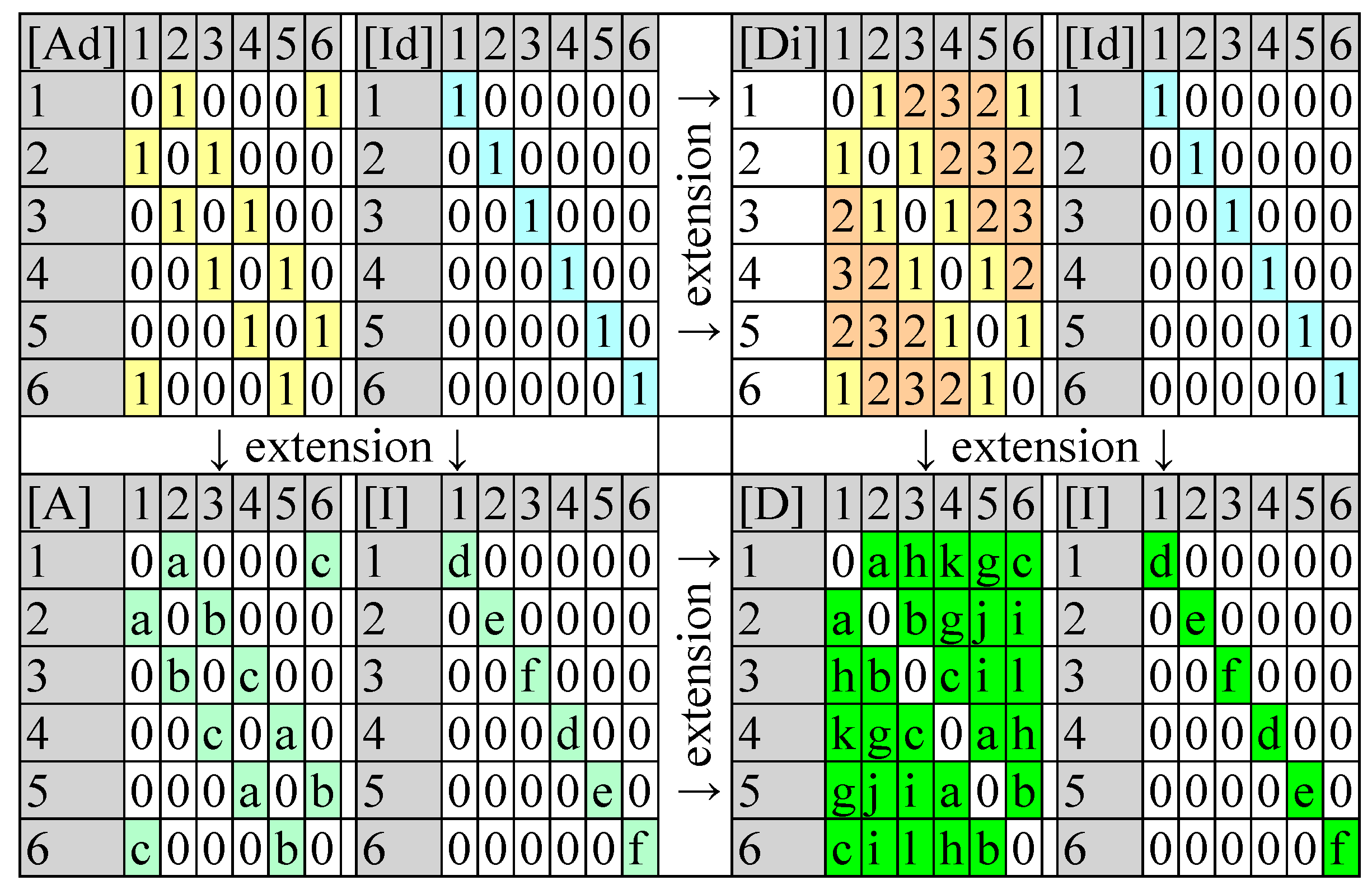
The full extension could include also the distance matrix (Figure 5).
The extended ChP has the following formula:
where [C] is either [A] or [D], the identities (a, b, and c from [I]) and the connectivity (d, e, f, g, h, i, j, k, and l from [C]).
ChP ← |λ × [I] − [C]|
The single-value entries (0 and 1 ≠ 0 for the classical definition of the ChP) can be upgraded to multi-value (any value), accounting for different atoms and bonds. Obviously, the classical ChP is found when a = b = c = d = e = f = 1 and g = h = i = j = k = l = 0.
Figure 6 shows the ChP extension differently accounting the identities from atomic properties ([I] ← AP ∈ {A, B, C, D, E, F, G, H, I, J, K, L}) and connectivity properties ([C] ← CP ∈ {t, g, c, b, T, G, C, B,}).
The extending characteristic polynomial (EChP) is designed for estimation/prediction of molecular properties, so a software implementation was done. EChP(λ, IP, CP) diverges as ChP(λ) does (to ∞) quickly with the increase of λ > 1. Thus, the [−1, 1] range → ‘2001′ grid is useful for evaluation. A linearization (LL) is required and was implemented since biological properties are expressed in log scale. The evaluation is performed at every point (out of 2001), requiring O(n3) operations (where n is the number of atoms).
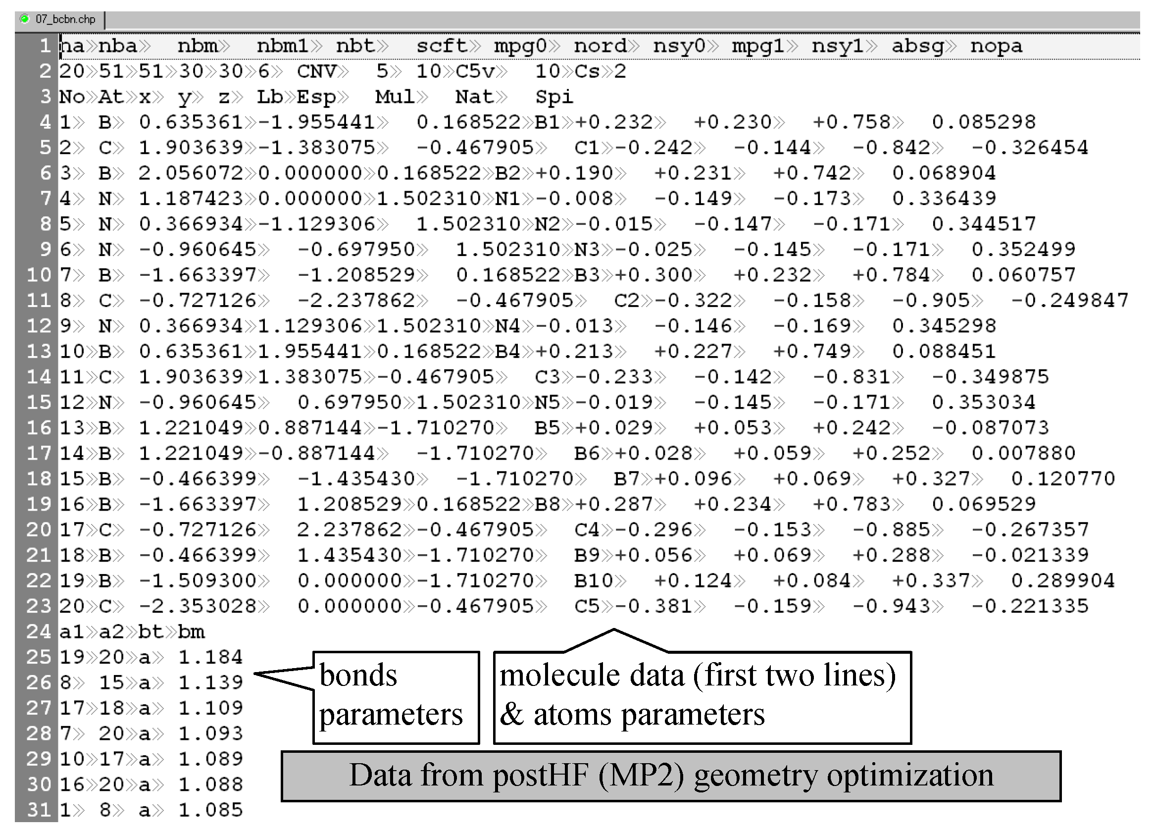
EChP is a family with 96 (nI*nC) polynomial formulas and 288 (*nL) linearized ones, leading to a total of 576,288 individuals. The FreePascal software was used for implementation since it is very fast and allows a parallelized version to be used with multi-CPUs (chp17chp.pas) [35]. The program requires input files in the ‘chp’ format (such as chfp_17_q.asc, see Figure 7), and uses a filtering (PHP) program (→chfp_17_t.asc) as well as a molecular property file (such as chfp_17 [prop].txt). The filtering program was designed to look for degenerations and to reduce the pool of descriptors by eliminating the degenerated ones.
The family of EChP descriptors was then used with a series of chemical compounds to obtain associations between the structure and properties as regression equations.
2.3. Numerical Case Study
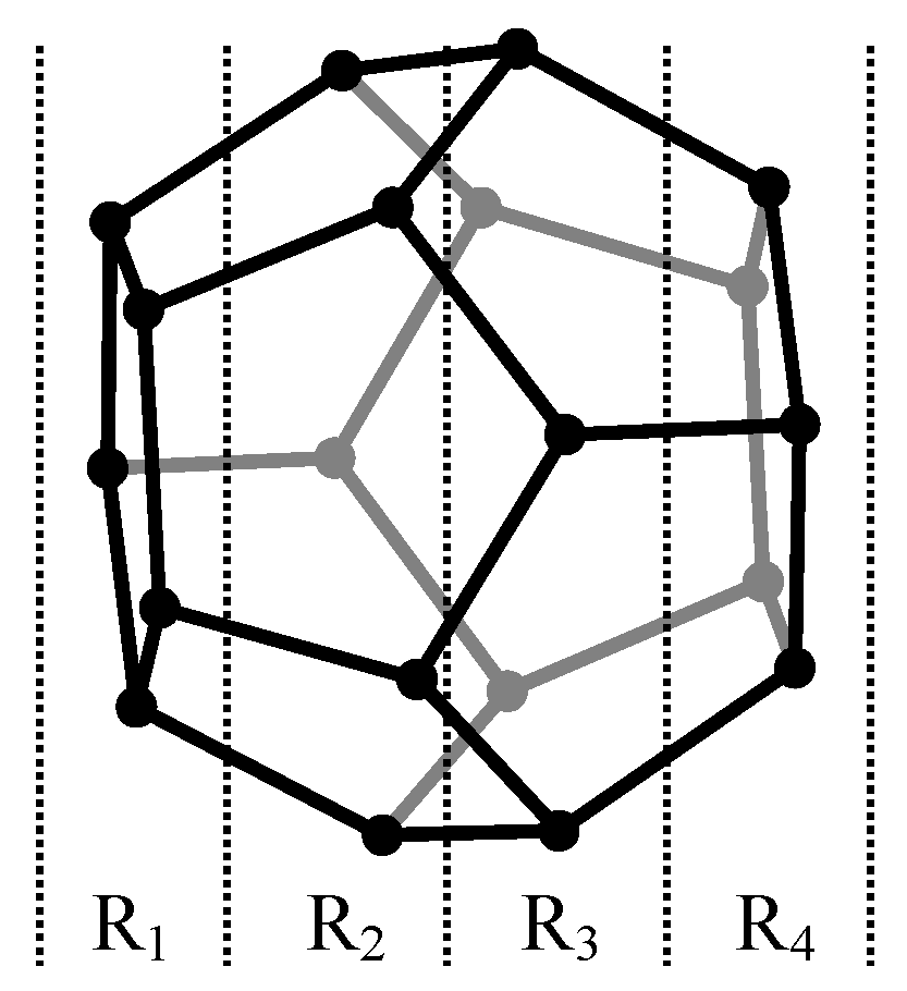
The case study was conducted on C20 fullerene congeners with Boron, Carbon, or Nitrogen atoms on each layer (Figure 8). A sample of 45 distinct compounds was obtained. The generic name of the files was stored as dd_R1R2R3R4, where dd is the number of the compound in the set and R1–R4 are the atoms on layers 1–4 (e.g., 02_bbbn.chp is the second compound in the sample and has boron of the first three layers and nitrogen on the last layer).
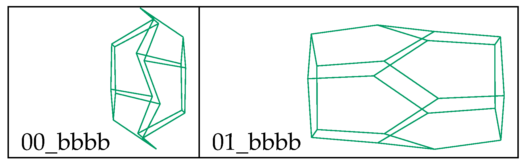
The geometries were built at the Hartree-Fock (HF) [3,4,5,6] 6-31 G [36] level of theory and calculated properties (namely, area and volume) were extracted from these calculations. Two different structures proved stable for bbbb (see Figure 9) and both were included in the analysis, resulting in a sample of 46 compounds.
The values of the calculated properties are given in Table 3.
Normal distribution of the data is one assumption that needs to be assessed before any linear regression analysis. Six different tests were used (AD = Anderson-Darling, KS = Kolmogorov-Smirnov, CM = Cramér-von Mises, KV = Kuiper V, WU = Watson U2, H1 = Shannon’s entropy [37]) [38] and the decision was made based on the combined test proposed by Fisher [39]. The distribution of the investigated properties proved to be not significantly different from the expected normal distribution (see Table 4, all p-values > 0.05).
Where for a series of cumulative distribution function values ((fi)1≤i≤n):
| Statistic | Formula |
| AD | |
| KS | |
| CM | |
| KV | |
| WU | |
| H1 | |
| FCS | ln(pAD·pKS·pCM·pKV·pWU·pH1) |
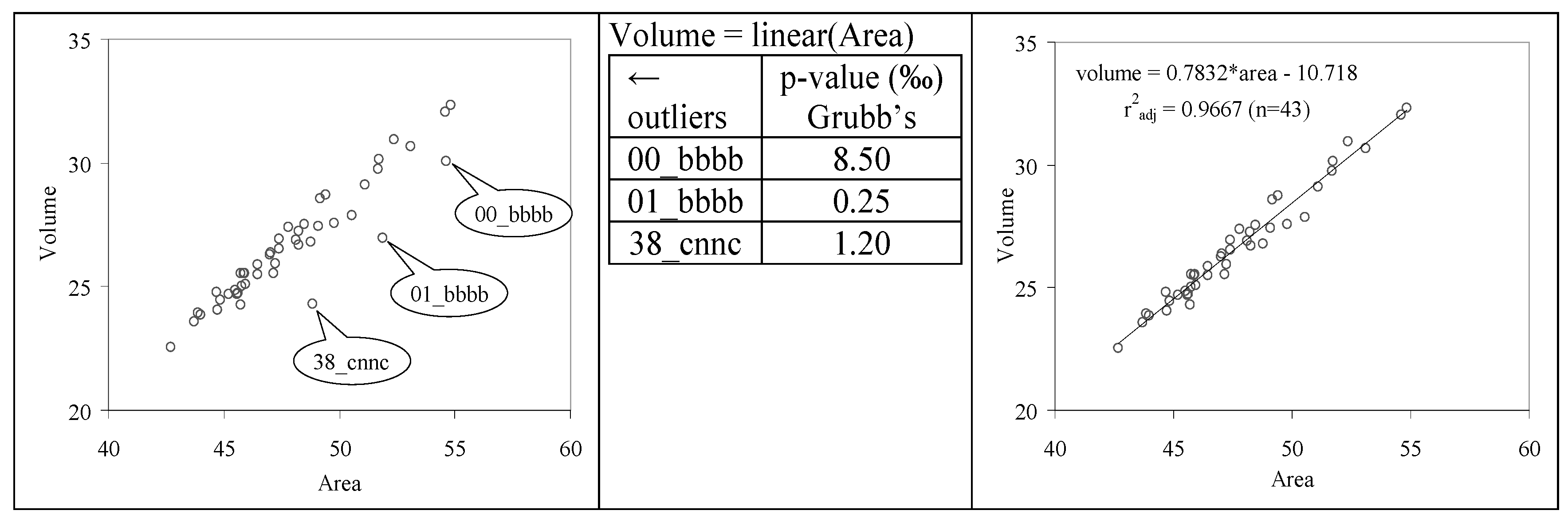
The absences of the outliers have also been investigated using Grubb’s test [40] for the association between volume (vol) and area on the sample of investigated C20 congeners. The analysis identified three compounds as outliers, their exclusion leading to a performing linear association (Figure 10).
The values of the EChP descriptors were generated for all molecules in the dataset and were used as input data for searching linear regression models able to explain the investigated properties (area and volume). Three different approaches were used, searching for additive, multiplicative, or full linear dependence (see Table 5).
The selection of the performing models was done using the adjusted determination coefficient (r2adj = r2 − (1 − r2)*kD*(n − kC)−1, where n is the number of compounds in the model). The difference between models with the same properties was tested using the studentized version of the Fisher Z transformation [41,42].
The best-performing models identified for the investigated properties are presented in Table 6 while the characteristics of the models are given in Table 7.
The relationship between volume and area is translated in the identification of the same EChP descriptors as the explanatory variable (two descriptors for additive models and one descriptor for multiplicative and respective full model, see Table 6). All models had a capacity of explanation higher than 85%, with the worst performance obtained by multiplicative models and similar performances (without significant difference) obtained by additive and full models (see Table 8).
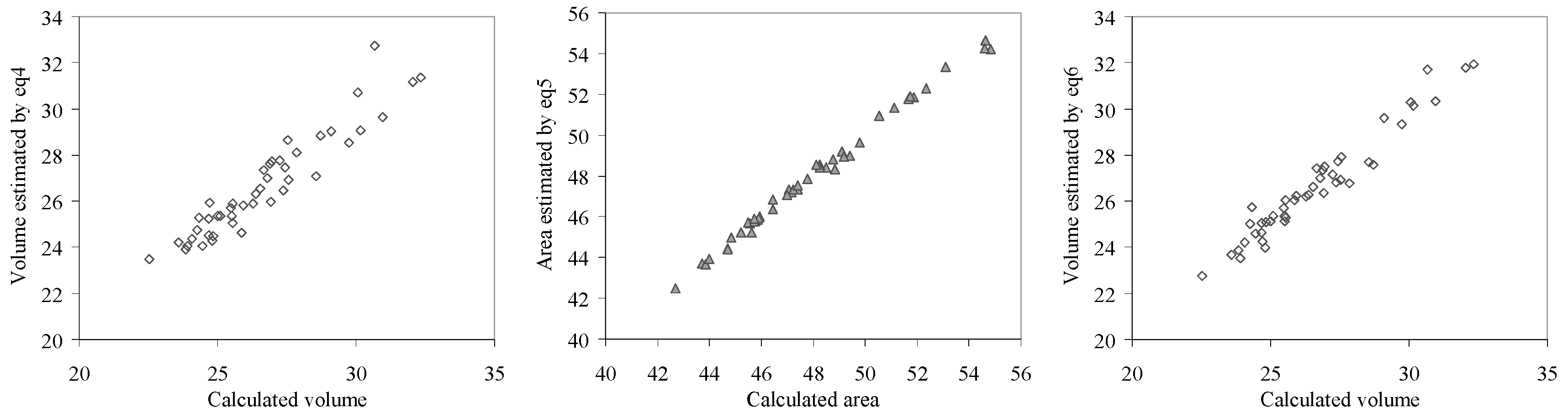
Graphical representations of calculated and estimated area and respective volume by the investigated effects are given in Figure 11 (eq1– eq3) and Figure 12 (eq4– eq6).
The model comparison strongly suggests that the best performing models are the additive or the full model for both investigated properties. However, since 03_bbcn is an outlier for the area on the additive model, we can say that choosing the full model will give a correct estimation.
It is important that the performing models identified using the EChP descriptors—the full model—select the same polynomial for both descriptors when both area and volume (”CG” in LCG+0.236, LCG+0.276, and LCG−0.908) are investigated. It should be noted that one descriptor is common for the estimation of the area and of the volume (LCG−0.908) for the C20 fullerene congeners. This fact, in conjunction with the higher correlation between volume and area (r2adj ≈ 0.97), the presence of outliers in one additive model, and the significant higher performance by full models in estimation sustained by goodness-of-fit and the graphical representation of calculated versus estimated, suggests that the best models are those with full effects.
3. Conclusions and Further Work
EChP proved useful for estimation of the investigated molecular properties. Both properties of C20 congeners—volume and area—are explained by a common descriptor (LCG−0.908 (or vice versa)).
EChP is a natural extension of the ChP. The scales of the atomic properties were more or less arbitrary selected and will be further investigated to find the optimal solution. Furthermore, the reversed distance seemed to be the best alternative but further analysis must be conducted to demonstrate this observation.
Author Contributions
Dan-Marian Joiţa made the molecules and supervised the molecular geometry optimization (energy minimization). Lorentz Jäntschi supervised the whole study and wrote the paper.
Conflicts of Interest
The authors declare no conflict of interest.
References
- Lagrange, J.-L. Sur L’équation Séculaire de la Lune; Mémoires de l’Acadéémie Royale des Science: Paris, France, 1773. [Google Scholar]
- Huckel, E. Quantentheoretische Beiträge zum Benzolproblem. Z. Phys. 1931, 70, 204–286. [Google Scholar] [CrossRef]
- Hartree, D.R. The Wave Mechanics of an Atom with a Non-Coulomb Central Field. Part I. Theory and Methods. Math. Proc. Camb. Philos. Soc. 1928, 24, 89–110. [Google Scholar] [CrossRef]
- Hartree, D.R. The Wave Mechanics of an Atom with a Non-Coulomb Central Field. Part II. Some Results and Discussion. Math. Proc. Camb. Philos. Soc. 1928, 24, 111–132. [Google Scholar] [CrossRef]
- Fock, V.A. Näherungsmethode zur Lösung des quantenmechanischen Mehrkörperproblems. Z. Phys. 1930, 61, 26–148. [Google Scholar] [CrossRef]
- Fock, V.A. “Selfconsistent field” mit Austausch für Natrium. Z. Phys. 1930, 62, 795–805. [Google Scholar] [CrossRef]
- Laplace, P.S. Recherches sur le Calcul Intégral et sur le Système du Monde; Mémoires 1’Académie des Sciences: Paris, France, 1776; Volume 2, pp. 47–179. [Google Scholar]
- Cauchy, A. Sur l’équation à l’aide de laquelle on détermine les inégalités séculaires des mouvements des planets. Exerc. Math. 1829, 4, 140–160. [Google Scholar]
- Slater, J.C. The Theory of Complex Spectra. Phys. Rev. 1929, 34, 1293–1295. [Google Scholar] [CrossRef]
- Hartree, D.R.; Hartree, W. Self-Consistent Field, with Exchange, for Beryllium. Proc. R. Soc. A Math. Phys. Eng. Sci. 1935, 50, 9–33. [Google Scholar] [CrossRef]
- Sylvester, J.J. On the theory connected with Newton’s rule for the discovery of imaginary roots of equations. Messenger Math. 1880, 9, 71–84. [Google Scholar]
- Godsil, C.D.; Gutman, I. On the theory of the matching polynomial. J. Graph Theory 1981, 5, 137–144. [Google Scholar] [CrossRef]
- Godsil, C.D. Algebraic Matching Theory. Electron. J. Comb. 1995, 2, #R8. [Google Scholar]
- Diudea, M.V.; Gutman, I.; Jäntschi, L. Molecular Topology; Nova Science: New York, NY, USA, 2001. [Google Scholar]
- Ramaraj, R.; Balasubramanian, K. Computer generation of matching polynimials of chemical graphs and lattices. J. Comput. Chem. 1985, 6, 122–141. [Google Scholar] [CrossRef]
- Curticapean, R. Counting Matchings of Size k Is # W[1]-Hard. In Proceedings of the 40th International Conference on Automata, Languages, and Programming, ICALP’13, Riga, Latvia, 8–12 July 2013; Volume 7965, pp. 352–363. [Google Scholar]
- Hosoya, H. Topological Index. A Newly Proposed Quantity Characterizing the Topological Nature of Structural Isomers of Saturated Hydrocarbons. Bull. Chem. Soc. Jpn. 1971, 44, 2332–2339. [Google Scholar] [CrossRef]
- Schöning, U. Graph isomorphism is in the low hierarchy. J. Comput. Syst. Sci. 1987, 37, 312–323. [Google Scholar] [CrossRef]
- King, R.B. Applications of graph theory and topology for the study of aromaticity in inorganic compounds. J. Chem. Inf. Model. 1992, 32, 42–47. [Google Scholar] [CrossRef]
- Santos, J.C.; Andres, J.; Aizman, A.; Fuentealba, P. An Aromaticity Scale Based on the Topological Analysis of the Electron Localization Function Including σ and π Contributions. J. Chem. Theory Comput. 2005, 1, 83–86. [Google Scholar] [CrossRef] [PubMed]
- Herndon, W.C. Structure-resonance theory for pericyclic transition states. J. Chem. Educ. 1981, 58, 371. [Google Scholar] [CrossRef]
- Bruderer, M.; Contreras-Pulido, L.D.; Thaller, M.; Sironi, L.; Obreschkow, D.; Plenio, M.B. Inverse counting statistics for stochastic and open quantum systems: The characteristic polynomial approach. New J. Phys. 2014, 16, 033030. [Google Scholar] [CrossRef]
- Arguin, L.-P.; Belius, D.; Bourgade, P. Maximum of the Characteristic Polynomial of Random Unitary Matrices. Commun. Math. Phys. 2017, 349, 703–751. [Google Scholar] [CrossRef]
- Da Lita Silva, J. On the characteristic polynomial, eigenvectors and determinant of heptadiagonal matrices. Linear Multilinear Algebra 2017, 65, 1852–1866. [Google Scholar] [CrossRef]
- Collatz, L.; Sinogowitz, U. Spektren Endlicher Grafen. Abh. Math. Semin. Univ. Hambg. 1957, 21, 63–77. [Google Scholar] [CrossRef]
- Sloane, N.J.A. Number of Graphs on n Unlabeled Nodes; A000088; On-Line Encyclopedia of Integer Sequences (OEIS): Highland Park, NJ, USA, 1996. [Google Scholar]
- Weisstein, W.E. Number of Unique Characteristic Polynomials among All Simple Undirected Graphs on n Nodes; A082104; On-Line Encyclopedia of Integer Sequences (OEIS): Highland Park, NJ, USA, 2003. [Google Scholar]
- McNaught, A. The IUPAC international chemical identifier. Chem. Int. 2006, 28, 12–15. [Google Scholar]
- Jäntschi, L.; Bolboacă, S.D.; Furdui, C.M. Characteristic and counting polynomials: Modelling nonane isomers properties. Mol. Simul. 2009, 35, 220–227. [Google Scholar] [CrossRef]
- Bolboacă, S.D.; Jäntschi, L. How good can the characteristic polynomial be for correlations? Int. J. Mol. Sci. 2007, 8, 335–345. [Google Scholar] [CrossRef]
- Jäntschi, L. Characteristic and Counting Polynomials of Nonane Isomers; Academic Direct Publishing House: Cluj-Napoca, Romania, 2007; ISBN 978-973-86211-3-8. [Google Scholar]
- Bolboacă, S.D.; Jäntschi, L. Characteristic Polynomial in Assessment of Carbon-Nano Structures. In Sustainable Nanosystems Development, Properties, and Applications; Putz, M.V., Mirica, M.C., Eds.; IGI Global: Hershey, PA, USA, 2017; pp. 122–147. ISBN 9781522504924. [Google Scholar]
- Bolboacă, S.D.; Jäntschi, L. Counting Distance and Szeged (on Distance) Polynomials in Dodecahedron Nano-assemblies. In Distance, Symmetry, and Topology in Carbon Nanomaterials; Ashrafi, A.R., Diudea, M.V., Eds.; Springer International Publishing: Cham, Switzerland, 2016; pp. 391–408. ISBN 978-3-319-31582-9. [Google Scholar]
- Jäntschi, L. Online Calculation of Graph Polynomials Such as Counting Polynomial and Characteristic Polynomial. 2006. Available online: http://l.academicdirect.org/Fundamentals/Graphs/polynomials/ (accessed on 21 January 2017).
- Gabor, B.M.; Vreman, P.P. Free Pascal: Open Source Compiler for Pascal and Object Pascal. 1988 (and to Date). Available online: http://freepascal.org (accessed on 21 January 2017).
- Hehre, W.J.; Ditchfield, R.; Pople, J.A. Self-consistent molecular orbital methods. XII. Further extensions of Gaussian-type basis sets for use in molecular orbital studies of organic molecules. J. Chem. Phys. 1972, 56, 2257–2261. [Google Scholar] [CrossRef]
- Jäntschi, L.; Bolboacă, S.D. Performances of Shannon’s Entropy Statistic in Assessment of Distribution of Data. Ovidius Univ. Ann. Chem. 2017, 28, 30–42. [Google Scholar] [CrossRef]
- Jäntschi, L. Tests. Available online: http://l.academicdirect.ro/Statistics/tests/ (accessed on 1 March 2017).
- Fisher, R.A. Questions and answers #14. Am. Stat. 1948, 2, 30–31. [Google Scholar]
- Bolboacă, S.D.; Jäntschi, L. Distribution Fitting 3. Analysis under Normality Assumptions. Bull. Univ. Agric. Sci. Vet. Med. Cluj-Napoca. Hortic. 2009, 66, 698–705. [Google Scholar]
- Student. The probable error of a mean. Biometrika 1908, 6, 1–25. [Google Scholar] [CrossRef]
- Welch, B.L. The generalization of student’s problem when several different population varlances are involved. Biometrika 1947, 34, 28–35. [Google Scholar] [CrossRef] [PubMed]
Figure 1.
Encoded identities [I], adjacencies [A] and distances [D]—an example.

Figure 2.
Graphs vs molecules—an example.

Figure 3.
Molecular geometry—an example.
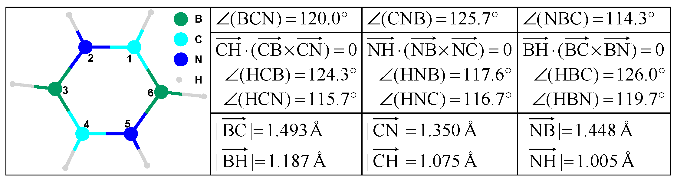
Figure 4.
Molecular geometry translated into adjacency and identity—an example.
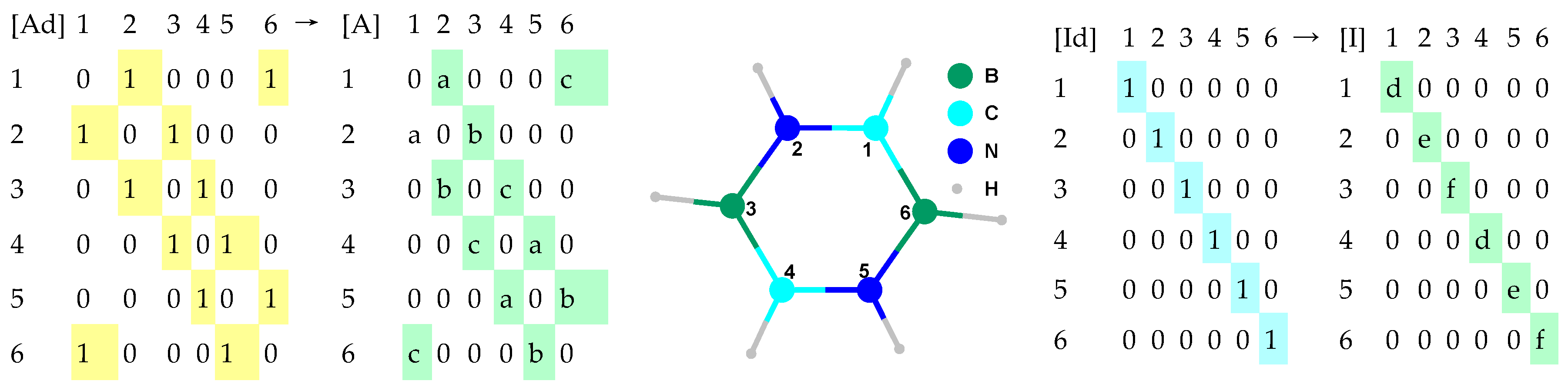
Figure 5.
Molecular geometry translated into adjacency, identity, and distance—an example.

Figure 6.
Extended characteristic polynomial—EChP.
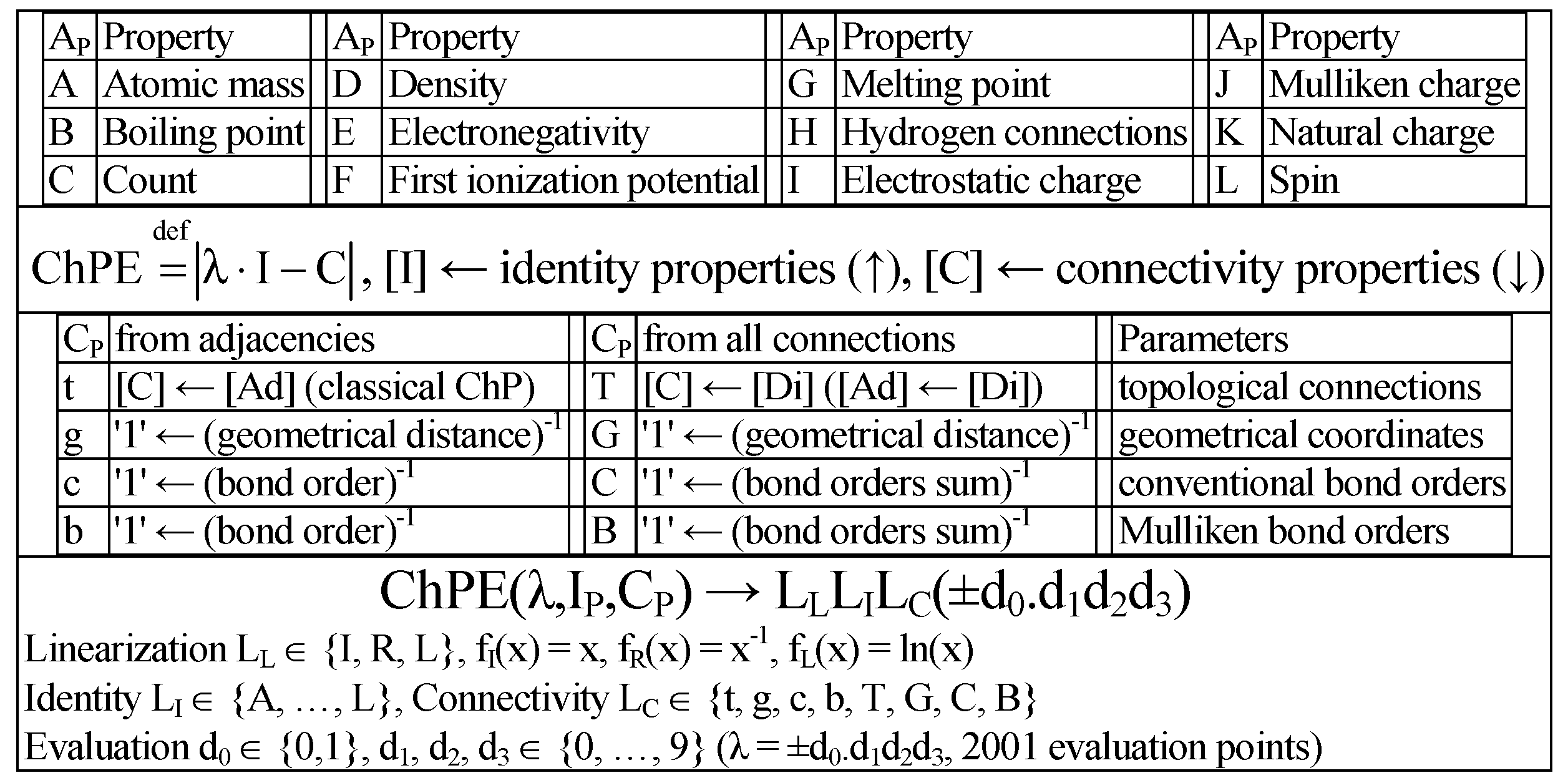
Figure 7.
EChP program: ‘chp’ input files, as an example.

Figure 8.
C20 fullerene congeners (R is the symbol of the atom on the layer).

Figure 9.
bbbb C20 stable fullerenes.

Figure 10.
Volume as linear function of area.

Figure 11.
Graphical representation of eq1–eq3 model performances.
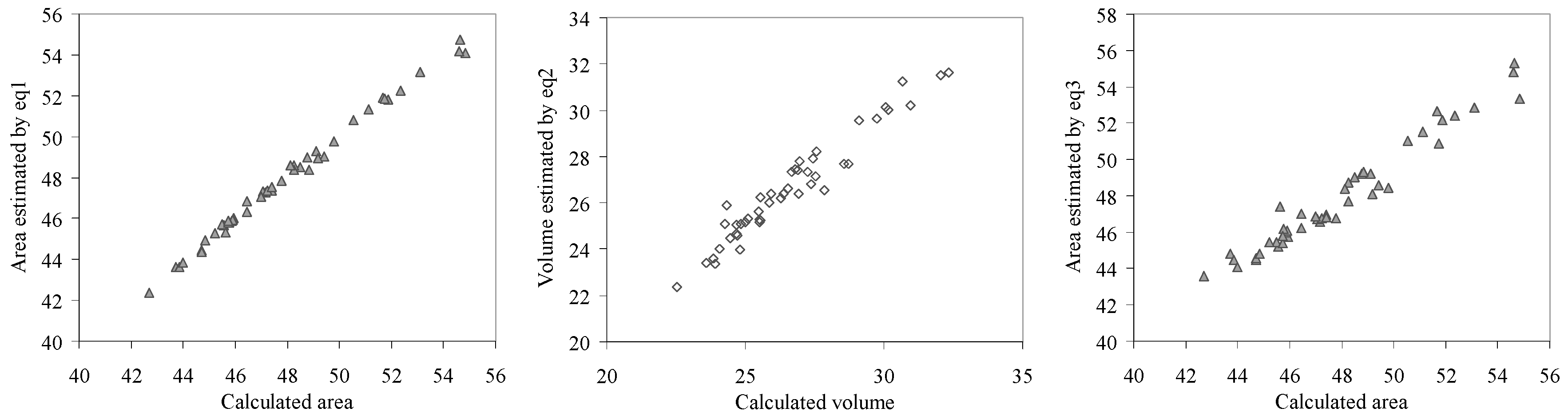
Figure 12.
Graphical representation of eq4– eq6 model performances.


Table 1.
Characteristic polynomial (ChP), Laplacian polynomial (LaP), Z-counting, and Matching Polynomials.
Table 1.
Characteristic polynomial (ChP), Laplacian polynomial (LaP), Z-counting, and Matching Polynomials.
| Name | Formula |
|---|---|
| ChP | |λ∙[Id] − [Ad]| |
| LaP | |λ∙[Id] − [Dg] + [Ad]| |
| Z-counting | Σk≥0 m(k)∙λk |
| Matching | Σk≥0 (−1)k∙m(k)∙λn−2k |
Table 2.
Classical molecular graphs.
| Definition | V: Finite Set | E ⊆ V × V | G = G(V,E) |
|---|---|---|---|
| Name (concept) | V: vertices (atoms) | E: edges (bonds) | G: graph (molecule) |
| Cardinality | |V| = n | |E| = m | ∀n, V ↔ {1, …, n} |
| Example | G = “A-B-C” | V = {1,2,3} | E = {(1,2), (2,3)} |
Table 3.
C20 congeners: values of investigated properties.
| Mol | Area | Volume | Mol | Area | Volume | Mol | Area | Volume |
|---|---|---|---|---|---|---|---|---|
| 00_bbbb | 54.641 | 30.063 | 16_cbbb | 50.537 | 27.863 | 31_ccnc | 42.689 | 22.542 |
| 01_bbbb | 51.863 | 26.948 | 17_cbbc | 51.114 | 29.107 | 32_ccnn | 43.987 | 23.862 |
| 02_bbbn | 54.848 | 32.333 | 18_cbbn | 49.097 | 27.424 | 33_cnbb | 49.186 | 28.569 |
| 03_bbcn | 48.481 | 27.524 | 19_cbcb | 51.733 | 30.156 | 34_cnbn | 44.694 | 24.794 |
| 04_bbnb | 53.093 | 30.658 | 20_cbcn | 47.401 | 26.543 | 35_cncb | 46.994 | 26.275 |
| 05_bbnn | 49.797 | 27.573 | 21_cbnb | 48.262 | 26.68 | 36_cncn | 44.723 | 24.062 |
| 06_bcbb | 54.597 | 32.043 | 22_cbnc | 45.944 | 25.109 | 37_cnnb | 45.76 | 24.995 |
| 07_bcbn | 49.415 | 28.726 | 23_cbnn | 45.578 | 24.689 | 38_cnnc | 48.834 | 24.315 |
| 08_bccb | 51.676 | 29.739 | 24_ccbb | 52.365 | 30.954 | 39_cnnn | 45.508 | 24.847 |
| 09_bccn | 47.392 | 26.933 | 25_ccbc | 45.618 | 24.718 | 40_nbbn | 48.119 | 26.881 |
| 10_bcnb | 48.782 | 26.786 | 26_ccbn | 45.857 | 25.514 | 41_nbnn | 45.726 | 24.275 |
| 11_bcnn | 47.15 | 25.543 | 27_cccb | 46.446 | 25.49 | 42_ncbn | 45.735 | 25.533 |
| 12_bnbn | 47.791 | 27.383 | 28_cccc | 43.707 | 23.584 | 43_nccn | 45.211 | 24.676 |
| 13_bncn | 47.048 | 26.368 | 29_cccn | 43.86 | 23.926 | 44_ncnn | 44.848 | 24.445 |
| 14_bnnb | 48.244 | 27.25 | 30_ccnb | 45.901 | 25.525 | 45_nnnn | 46.463 | 25.872 |
| 15_bnnn | 47.226 | 25.93 | - | - | - | - | - | - |
Table 4.
C20 congeners: values of investigated properties. AD = Anderson–Darling; KS = Kolmogorov–Smirnov; CM = Cramér–von Mises; KV = Kuiper V; WU = Watson U2; H1 = Shannon’s entropy.
Table 4.
C20 congeners: values of investigated properties. AD = Anderson–Darling; KS = Kolmogorov–Smirnov; CM = Cramér–von Mises; KV = Kuiper V; WU = Watson U2; H1 = Shannon’s entropy.
| Prop. | Title | AD | KS | CM | KV | WU | H1 | FCS(6) |
|---|---|---|---|---|---|---|---|---|
| area | stat | 0.826 | 0.758 | 0.131 | 1.213 | 0.110 | 22.83 | 3.660 |
| p | 0.462 | 0.423 | 0.548 | 0.552 | 0.770 | 0.565 | 0.723 | |
| volume | stat | 0.845 | 0.791 | 0.133 | 1.272 | 0.108 | 22.95 | 3.503 |
| p | 0.445 | 0.477 | 0.552 | 0.633 | 0.765 | 0.525 | 0.744 |
Table 5.
Approaches in bivariate (kD = 2) regression analysis.
| Y ~ Ŷ = a0 + a1*ChPE1 + a2*ChPE2 + a3*ChPE1*ChPE2 | ||
|---|---|---|
| Effect | Coefficient Constraints | kC |
| Additive (“+”) | a0 = 0, a1 ≠ 0, a2 ≠ 0, a3 = 0 | 2 (a1, a2) |
| a0 ≠ 0, a1 ≠ 0, a2 ≠ 0, a3 = 0 | 3 (a0, a1, a2) | |
| Multiplicative (“*”) | a0 = 0, a1 = 0, a2 = 0, a3 ≠ 0 | 1 (a3) |
| a0 ≠ 0, a1 = 0, a2 = 0, a3 ≠ 0 | 2 (a0, a3) | |
| Full | a0 = 0, a1 ≠ 0, a2 ≠ 0, a3 ≠ 0 | 3 (a1, a2, a3) |
| a0 ≠ 0, a1 ≠ 0, a2 ≠ 0, a3 ≠ 0 | 4 (a0, a1, a2, a3) | |
Table 6.
ChPE models.
| Eff | P | Model | eq |
|---|---|---|---|
| “+” | A | 35.8±0.3 − 8.2±0.1 * LCG+0.238 + 1.4±0.3 * LCG−0.896 | 1 a |
| V | 21.6±2.0 − 7.4±0.7 * LCG+0.238 + 1.7±0.3 * LCG−0.896 | 2 | |
| “*” | A | 34.0±0.9 + 0.16±0.01 * LEG+0.436 * LFG−0.952 | 3 |
| V | 17.6±1.0 + 0.101±0.011*LEG+0.436 * LCG−0.384 | 4 | |
| Full | A | 50.4±0.5 − 6.36±0.06 * LCG+0.276 + 2.3±0.5 * LCG-0.908 + 0.13±0.06 * LCG+0.276 * LCG−0.908 | 5 |
| V | 64±17 − 2.5±1.9 * LCG+0.236 + 4.5±1.2 * LCG-0.908 + 0.35±0.14 * LCG+0.236 * LCG−0.908 | 6 |
Eff = Effect; “+” = additive model; “*” = multiplicative model; P = property: A = Area, V = Volume. a 03_bbcn excluded outlier.
Table 7.
Model characteristics.
| Eff | P | eq | r2adj | se | F (p-Value) |
|---|---|---|---|---|---|
| “+” | A | 1 | 0.9934 | 0.2487 | 3386 (5.01 × 10−48) |
| V | 2 | 0.9385 | 0.5767 | 344 (3.41 × 10⁻²⁷) | |
| “*” | A | 3 | 0.9462 | 0.6575 | 931 (3.06 × 10⁻³¹) |
| V | 4 | 0.8894 | 0.7651 | 372 (4.37 × 10⁻²³) | |
| Full | A | 5 | 0.9940 | 0.2406 | 2413 (5.04 × 10−47) |
| V | 6 | 0.9462 | 0.5458 | 258 (4.37 × 10⁻²⁷) |
Eff = Effect; “+” = additive model; “*” = multiplicative model; P = property: A = Area, V = Volume, r2adj = adjusted determination coefficient; se = standard error of estimate, F (p-value) = Fisher’s statistic (associated significance).
Table 8.
Fisher’s Z model comparisons: results.
| Prop. | Parameter | “*” vs “+” | “*” vs Full | “+” vs Full |
|---|---|---|---|---|
| Area | Stat | 4.61 | 4.82 | 0.21 |
| p-value | <0.0001 | <0.0001 | 0.4176 | |
| Volume | Stat | 1.42 | 1.74 | 0.32 |
| p-value | 0.0791 | 0.0425 | 0.3752 |
© 2017 by the authors. Licensee MDPI, Basel, Switzerland. This article is an open access article distributed under the terms and conditions of the Creative Commons Attribution (CC BY) license (http://creativecommons.org/licenses/by/4.0/).
Share and Cite
MDPI and ACS Style
Joiţa, D.-M.; Jäntschi, L. Extending the Characteristic Polynomial for Characterization of C20 Fullerene Congeners. Mathematics 2017, 5, 84. https://doi.org/10.3390/math5040084
AMA Style
Joiţa D-M, Jäntschi L. Extending the Characteristic Polynomial for Characterization of C20 Fullerene Congeners. Mathematics. 2017; 5(4):84. https://doi.org/10.3390/math5040084
Chicago/Turabian StyleJoiţa, Dan-Marian, and Lorentz Jäntschi. 2017. "Extending the Characteristic Polynomial for Characterization of C20 Fullerene Congeners" Mathematics 5, no. 4: 84. https://doi.org/10.3390/math5040084
Note that from the first issue of 2016, this journal uses article numbers instead of page numbers. See further details here.