Global Dynamics of Certain Mix Monotone Difference Equation


1
Department of Mathematics, University of Sarajevo, 71000 Sarajevo, Bosnia and Herzegovina
2
Department of Mathematics, University of Tuzla, 75000 Tuzla, Bosnia and Herzegovina
*
Author to whom correspondence should be addressed.
Mathematics 2018, 6(1), 10; https://doi.org/10.3390/math6010010
Submission received: 7 December 2017
/
Revised: 3 January 2018
/
Accepted: 7 January 2018
/
Published: 12 January 2018
(This article belongs to the Special Issue Advances in Differential and Difference Equations with Applications)
Abstract
:We investigate global dynamics of the following second order rational difference equation where the parameters are positive real numbers and initial conditions and are arbitrary positive real numbers. The map associated to the right-hand side of this equation is always decreasing in the second variable and can be either increasing or decreasing in the first variable depending on the corresponding parametric space. In most cases, we prove that local asymptotic stability of the unique equilibrium point implies global asymptotic stability.
Keywords:
difference equations; equilibrium; period-two solutions; period-four solutions; global stability; monotonicityMSC:
39A10; 39A20; 39A23; 39A301. Introduction and Preliminaries
In this paper, we investigate the local and global character of the equilibrium point of the following second order rational difference equation
where the parameters are nonnegative real numbers and initial conditions and are arbitrary nonnegative real numbers, such that , .
Equation (1) is the special case of a general second order quadratic rational difference equation of the form
with nonnegative parameters and nonegative initial conditions such that , and , . Several global asymptotic results for some special cases of Equation (2) were obtained in [1,2,3,4,5,6,7,8,9,10,11].
One interesting special case by (2) is the following rational difference equation studied in [12]:
which represents discretization of the differential equation model in biochemical networks, see [13]. Notice that Equation (3) is an example of a rational difference equation, such that associated map is always strictly decreasing with respect to the second variable, and changes its monotonicity with respect to the first variable, i.e., can be increasing or decreasing depending on corresponding parametric space. Also, we see that Equation (3) is the special case of the linear rational difference equation
(which was investigated in detail in [12]) with well known and complicated dynamics, such as Lynes’ equation (see [14]).
There are not many papers that study in detail dynamics of the second order rational difference equations with quadratic terms such that associated map changes its monotonicity with respect to its variables. However, in [15] the behavior of the following rational difference equation has been investigated in great detail
In both equations, (3) and (5), Theorems 1 and 2 were used in order to obtain the convergence results. In most cases of this paper we use the same results. However, in order to investigate the behaviour of the following four subsequences , , , that appears under the condition where we cannot use this method, because the associated map in this case does not have the same monotonicity with respect to its variables in invariant interval. More precisely, the corresponding map changes its monotonicity in invariant interval with respect to the first variable. Instead of that, we use the brute-force method to show that each subsequence converges to the unique equilibrium point.
In the case when associated map of Equation (1) changes its monotonicity from “decreasing-decreasing” into “increasing-decreasing”, the problem of determining invariant interval appears. In all cases, we determine invariant interval and prove that the positive equilibrium of Equation (1), which is always locally asymptotically stable, is globally asymptotically stable for all values of the parameters, except in the case when (see Theorems 7–10).
The problem of determining invariant intervals in the case when the associated map changes its monotonicity with respect to its variables has been considered in [16,17]. Also, see [18,19,20].
Now, we state several well-known results.
Theorem 1.
[14] [Theorem 2.22] Let be an interval, and suppose that is a continuous function. Consider the difference equation
Assume that f satisfies the following two conditions:
a. is nondecreasing in for each , and is nonincreasing in for each ;
b. All solutions of the system
satisfy .
Theorem 2.
[12] [Theorem 1.4.7] Let be an interval, and suppose that is a continuous function satisfying the following properties:
a. is nonincreasing in each of its arguments;
b. If is a solution of the system
then .
Theorem 3.
- 1.
- ;
- 2.
- is nonincreasing in u and v respectively;
- 3.
- is nondecreasing in x;
- 4.
- Equation (6) has a unique positive equilibrium .
Then, every positive solution of Equation (6) which is bounded from above and from below by positive constants converges to .
Theorem 4.
[12] [Theorem 1.7.2] Assume that and that is decreasing in both arguments.
Theorem 5.
[12] [Theorem 1.7.4] Assume that is such that: is increasing in x for each fixed y, and is decreasing in y for each fixed x.
2. Linearized Stability
In this section, we prove that Equation (1) has a unique equilibrium point which is always locally asymptotically stable.
The equilibrium point of Equation (1) satisfies
Theorem 6.
Proof.
The real function associated to Equation (1) is given by
We have that the function is always decreasing with respect to the second variable and can be either decreasing or increasing with respect to the first variable, depending on the sign of nominator, that is depending on corresponding parametric space. Now, we check the conditions of Theorem 1.1.1, see [12]. The condition becomes
The second inequality is equivalent to , which is always true. The first inequality becomes
Now, we have
which is always true.
Also, we have
which is always true. □
Lemma 1.
Every solution of Equation (1) is bounded.
Proof.
From Equation (1), we have
which completes the proof. □
Lemma 2.
Equation (1) does not posses a minimal period-two solution.
Proof.
Period-two solution satisfies the following system of algebraic equations
By replacing the function we have
By subtracting these two equations, we obtain
If , then there does not exist a minimal period-two solution. However, if , we have
3. Global Attractivity Results
In this section, we prove several global attractivity results in the corresponding parametric space.
We notice that the sign of the partial derivative with respect to the first variable at the equilibrium point depends on the sign of the .
, In this case, the function f is increasing in the first variable and decreasing in the second variable.
Lemma 3.
If or or , then the system of algebraic equations
has a unique solution .
Proof.
If , then system (13) has a unique solution .
Suppose that and . Then
Now, we see that Equation (17) has no positive solutions if This means that system (13) has a unique solution in this case.
It is easy to see that when , which means that system (13) has a unique solution in this case. Similarly, if , then .
Finally, if , then system (13) has more than one positive solution. □
Theorem 7.
Assume that one of the following conditions hold:
- (1)
- (2)
Proof.
In this case (see the proof of Lemma 1) the invariant interval (and an attracting interval) of Equation (1) is
Since , then f is increasing in the first variable and decreasing in the second variable and we can apply Theorem 1. Also, we know that the equilibrium is locally asymptotically stable, and consequently the proof will be completed by using Lemma 3 and Theorem 1. □
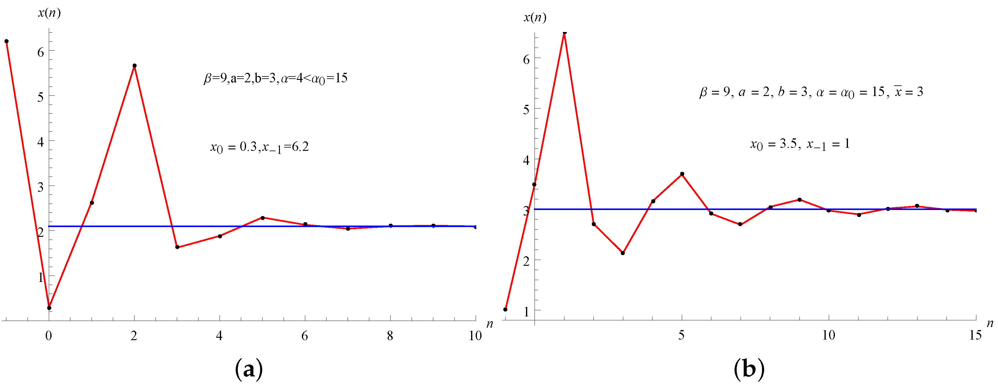
For some numerical values of parameters we give visual evidence for Theorem 7. (See Figure 1a).
, Lemma 1 implies that
Now, we have
Since
we have to consider the following three cases:
- (i)
- (ii)
- (iii)
For the case of we have the following result about global behavior of solutions of Equation (1).
Theorem 8.
Assume that one of the following conditions hold:
- (1)
- (2)
Proof.
Since , we have that , i.e., from which
In this case we have
which implies that the interval is an invariant interval. Indeed, since the function is continuous, then attains its extreme points at the end of closed interval or at the stationary point. Straightforward calculations show that all values
are in
Set
We know that On the other hand, we have that
which implies .
Also, we know that , which implies that f is increasing in the first variable and decreasing in the second variable. Since Equation (1) has the unique equilibrium point in invariant interval , we can apply Theorem 1. Also, we know that the equilibrium is locally asymptotically stable, and consequently the proof will be completed by using Lemma 3 and Theorem 1. □
For some numerical values of parameters we give visual evidence for Theorem 8. (See Figure 1b).
For the case of the following result holds.
Theorem 9.
Proof.
Since , then , that is , from which .
First, we prove that the invariant interval is given by . Since the function is continuous, then this function attains its extreme points at the end of closed interval or at the stationary point. Straightforward calculations show that
are in .
Now, we prove that the equilibrium point is in interval . Set
We know that On the other hand, we have
which shows that .
Since the function is decreasing in both variables, and Equation (1) has the unique equilibrium point in invariant interval , we can apply Theorem 2. System of algebraic equations
becomes
It is easy to see that this system has a unique solution , which completes the proof. □
For some numerical values of parameters we give visual evidence for Theorem 9. (See Figure 2a).
Remark 1.
Notice that we can prove Theorem 9 by using Theorem 3. In this case, we have
which means that every solution of Equation (1) is bounded from above and from below by positive constants.
Since
and f clearly satisfies the conditions 1. and 2. of Theorem 3. Now, by using Theorem 3, we have that every solution of Equation (1) converges to .
Now, consider the case .
Lemma 4.
Assume that , that is , where . Then, Equation (1) does not posses a minimal period-four solution.
Proof.
Suppose the opposite, i.e., Equaiton (1) has a minimal period-four solution: , that is the following equalities hold
By eliminating z and t we obtain
where
Theorem 10.
Proof.
After straightforward calculations, we obtain
From (19) we have
On the other hand,
if and only if
which is true.
Therefore, for , we have that
and we see that and are always on the same side of the equilibrium point . Namely, if , then
and so, if , then
Therefore, every sequence , , , is monotone and bounded. This implies that each of the sequences is convergent. Since, by Lemma 4, Equation (1) has no minimal period-four solutions, we have that
which implies that the equilibrium is an attractor. It means that is globally asymptotically stable. □
For some numerical values of parameters we give visual evidence for Theorem 10. (See Figure 2b)
Remark 2.
Notice that in the case when these four subsequences exist, there is an invariant interval of this form , but we can not use any of Theorems 1 and 2 because the map associated with Equation (1) changes its monotonicity with respect to the first variable in this invariant interval.
Remark 3.
Also, based on our numerical simulations, we give the following conjecture.
Author Contributions
All three authors have significant contribution to this paper and the final form of this paper is approved by all three authors.
Conflicts of Interest
The authors declare no conflict of interest.
References
- Bektešević, J.; Hadžiabdić, V.; Kalabušić, S.; Mehuljić, M. Global Asymptotic Behavior of Some Quadratic Rational Second-Order Difference Equations. Int. J. Differ. Equ. 2017, 12, 169–183. [Google Scholar]
- Garić-Demirović, M.; Kulenović, M.R.S.; Nurkanović, M. Global Dynamics of Certain Homogeneous Second-Order Quadratic Fractional Difference Equations. Sci. World J. 2013, 2013, 10. [Google Scholar] [CrossRef] [PubMed]
- Garić-Demirović, M.; Kulenović, M.R.S.; Nurkanović, M. Basins of Attraction of Certain Homogeneous Second Order Quadratic Fractional Difference Equation. J. Concr. Appl. Math. 2015, 13, 35–50. [Google Scholar]
- Garić-Demirović, M.; Nurkanović, M.; Nurkanović, Z. Stability, Periodicity and Neimark–Sacker Bifurcation of Certain Homogeneous Fractional Difference Equations. Int. J. Differ. Equ. 2017, 12, 27–53. [Google Scholar]
- Hrustić, S.J.; Kulenović, M.R.S.; Nurkanović, M. Global Dynamics and Bifurcations of Certain Seond Order Rational Difference Equation with Quadratic Terms. Qual. Theory Dyn. Syst. 2016, 15, 283. [Google Scholar] [CrossRef]
- Jašarević-Hrustić, S.; Nurkanović, Z.; Kulenović, M.R.S.; Pilav, E. Birkhoff normal forms, KAM theory and symmetries for certain second order rational difference equation with quadratic term. Int. J. Differ. Equ. 2015, 10, 181–199. [Google Scholar]
- Kent, C.M.; Sedaghat, H. Global attractivity in a quadratic-linear rational difference equation with delay. J. Differ. Equ. Appl. 2009, 15, 913–925. [Google Scholar] [CrossRef]
- Kent, C.M.; Sedaghat, H. Global attractivity in a rational delay difference equation with quadratic terms. J. Differ. Equ. Appl. 2011, 17, 457–466. [Google Scholar] [CrossRef]
- Kulenović, M.R.S.; Moranjkić, S.; Nurkanović, Z. Naimark-Sacker Bifurcation of Second Order Rational Difference Equation with Quadratic Terms. J. Nonlinear Sci. Appl. 2017, 10, 3477–3489. [Google Scholar] [CrossRef]
- Moranjkić, S.; Nurkanović, Z. Local and Global Dynamics of Certain Second-Order Rational Difference Equations Containing Quadratic Terms. Adv. Dyn. Syst. Appl. 2017, 12, 123–157. [Google Scholar]
- Sedaghat, H. Global behaviours of rational difference equations of orders two and three with quadratic terms. J. Differ. Equ. Appl. 2009, 15, 215–224. [Google Scholar] [CrossRef]
- Kulenović, M.R.S.; Ladas, G. Dynamics of Second Order Rational Difference Equations with Open Problems and Conjectures; Chapman and Hall/CRC: Boca Raton, FL, USA; London, UK, 2001. [Google Scholar]
- Enciso, E.G.; Sontag, E.D. Global attractivity, I/O monotone small-gain theorems, and biological delay systems. Discrete Contin. Dyn. Syst. 2006, 14, 549–578. [Google Scholar]
- Kulenović, M.R.S.; Merino, O. Discrete Dynamical Systems and Difference Equations with Mathematica; Chapman and Hall/CRC Press: Boca Raton, FL, USA, 2002. [Google Scholar]
- Kostrov, Y.; Kudlak, Z. On a Second-Order Rational Difference Equation with a Quadratic Term. Int. J. Differ. Equ. 2016, 11, 179–202. [Google Scholar]
- Kulenović, M.R.S.; Nurkanović, M. Asymptotic behavior of a two dimensional linear fractional system of difference equations. Radovi Matematički 2002, 11, 59–78. [Google Scholar]
- Kulenović, M.R.S.; Nurkanović, M. Asymptotic Behavior of a Linear Fractional System of Difference Equations. J. Inequal. Appl. 2005, 127–143. [Google Scholar] [CrossRef]
- Burgić, D.; Kulenović, M.R.S.; Nurkanović, M. Global Dynamics of a Rational System of Difference Equations in the plane. Commun. Appl. Nonlinear Anal. 2008, 15, 71–84. [Google Scholar]
- Moranjkić, S.; Nurkanović, Z. Basins of attraction of certain rational anti-competitive system of difference equations in the plane. Adv. Differ. Equ. 2012, 2012, 153. [Google Scholar] [CrossRef]
- Smith, H.L. Non-monotone systems decomposable into monotone systems with negative feedback. J. Math. Biol. 2006, 53, 747–758. [Google Scholar] [CrossRef] [PubMed]
- Drymonis, E.; Ladas, G. On the global character of the rational system . Sarajevo J. Math. 2012, 8, 293–309. [Google Scholar] [CrossRef]
Figure 1.
Numerical simulation of stability for: (a) ; (b) and .
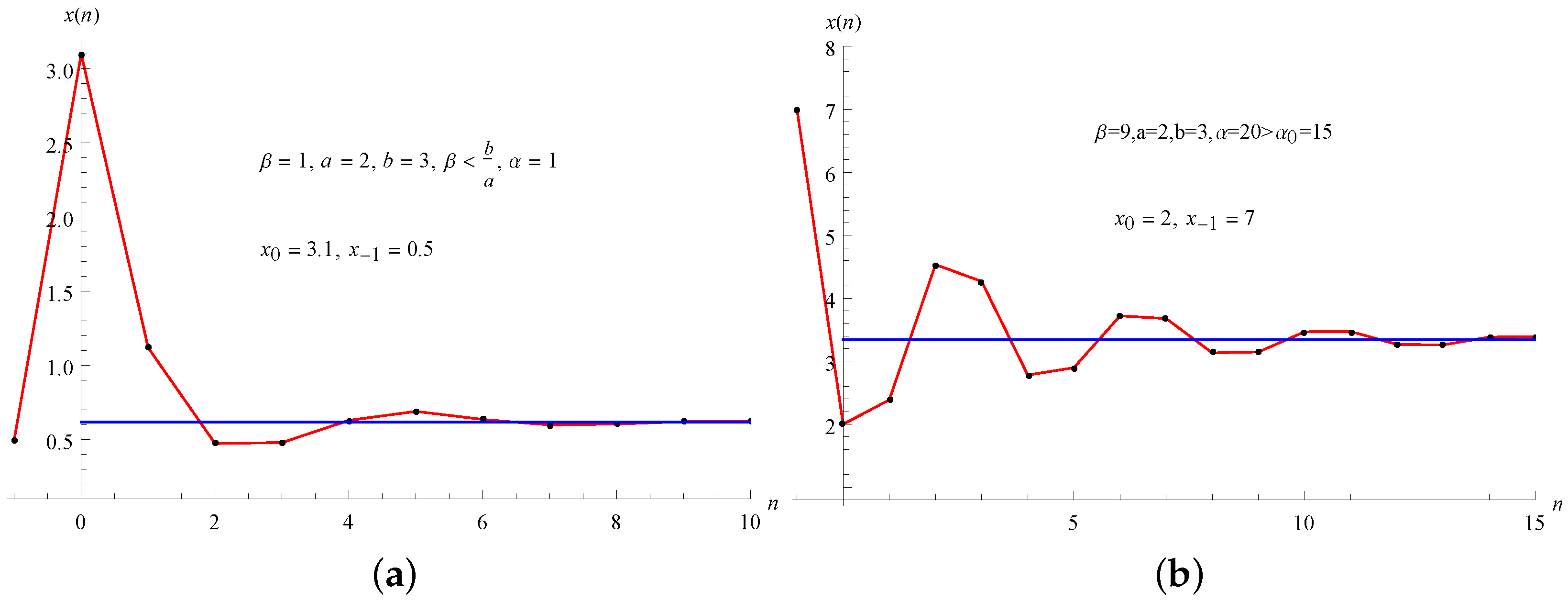
Figure 2.
Numerical simulation of stability for (a) ; (b) .

© 2018 by the authors. Licensee MDPI, Basel, Switzerland. This article is an open access article distributed under the terms and conditions of the Creative Commons Attribution (CC BY) license (http://creativecommons.org/licenses/by/4.0/).
Share and Cite
MDPI and ACS Style
Kalabušić, S.; Nurkanović, M.; Nurkanović, Z. Global Dynamics of Certain Mix Monotone Difference Equation. Mathematics 2018, 6, 10. https://doi.org/10.3390/math6010010
AMA Style
Kalabušić S, Nurkanović M, Nurkanović Z. Global Dynamics of Certain Mix Monotone Difference Equation. Mathematics. 2018; 6(1):10. https://doi.org/10.3390/math6010010
Chicago/Turabian StyleKalabušić, Senada, Mehmed Nurkanović, and Zehra Nurkanović. 2018. "Global Dynamics of Certain Mix Monotone Difference Equation" Mathematics 6, no. 1: 10. https://doi.org/10.3390/math6010010
Note that from the first issue of 2016, this journal uses article numbers instead of page numbers. See further details here.