Notions of Rough Neutrosophic Digraphs


1
Department of Mathematics, University of the Punjab, New Campus, Lahore 54590, Pakistan
2
Department of Mathematics & Science, University of New Mexico, 705 Gurley Ave., Gallup, NM 87301, USA
*
Author to whom correspondence should be addressed.
Mathematics 2018, 6(2), 18; https://doi.org/10.3390/math6020018
Submission received: 7 December 2017
/
Revised: 19 January 2018
/
Accepted: 23 January 2018
/
Published: 29 January 2018
Abstract
:Graph theory has numerous applications in various disciplines, including computer networks, neural networks, expert systems, cluster analysis, and image capturing. Rough neutrosophic set (NS) theory is a hybrid tool for handling uncertain information that exists in real life. In this research paper, we apply the concept of rough NS theory to graphs and present a new kind of graph structure, rough neutrosophic digraphs. We present certain operations, including lexicographic products, strong products, rejection and tensor products on rough neutrosophic digraphs. We investigate some of their properties. We also present an application of a rough neutrosophic digraph in decision-making.
1. Introduction
There are many real-life problems that are beyond a single expert. These are because of the need to involve a wide domain of knowledge. As a generalization of the intuitionistic fuzzy set, a neutrosophic set (NS) has been introduced by Smarandache [1]. This is a useful tool to deal with uncertainty in several social and natural aspects. Neutrosophy provides a foundation for a whole family of new mathematical theories with the generalization of both classical and fuzzy counterparts. In a NS, an element has three associated defining functions, the truth membership function (), the indeterminate membership function () and the false membership function (), defined on a universe of discourse X. These three functions are completely independent. To apply NSs in real-life problems more conveniently, Smarandache [2] and Wang et al. [3] defined single-valued NSs. Ye [4] studied the correlation coefficient and improved the correlation coefficient of NSs, as well as determined that in NSs the cosine similarity measure is a special case of the correlation coefficient.
Rough set theory was proposed by Pawlak [5] in 1982. Rough set theory is useful to study the intelligence systems containing incomplete, uncertain or inexact information. The lower and upper approximation operators of rough sets are used for managing hidden information in a system. Therefore, many hybrid models have been built, such as soft rough sets, rough fuzzy sets, fuzzy rough sets, soft fuzzy rough sets, neutrosophic rough sets, and rough NSs for handling uncertainty and incomplete information effectively. Dubois and Prade [6] introduced the notions of rough fuzzy sets and fuzzy rough sets. Liu and Chen [7] have studied different decision-making methods. Broumi et al. [8] introduced the concept of rough NSs. Yang et al. [9] proposed single-valued neutrosophic rough sets by combining single-valued NSs and rough sets, and they established an algorithm for decision-making problems based on single-valued neutrosophic rough sets on two universes. Mordeson and Peng [10] presented operations on fuzzy graphs. Akram et al. [11,12,13,14] considered several new concepts of neutrosophic graphs with applications. Zafer and Akram [15] dealt with rough fuzzy digraphs with applications. Recently, Sayed et al. [16] considered rough neutrosophic digraphs. They discussed some fundamental properties of rough neutrosophic digraphs. In this research paper, we investigate further new operations, including lexicographic products, strong products, rejection and tensor products on rough neutrosophic digraphs. We investigate some of their properties. We also consider an application of a rough neutrosophic digraph in decision-making.
2. Rough Neutrosophic Digraphs
For other notations, terminologies and applications not mentioned in the paper, the readers are referred to [17,18,19,20,21].
Definition 1.
[3] Let Z be a nonempty universe. A NS N on Z is defined as follows:
where the functions :Z→ represent the degree of membership, the degree of indeterminacy and the degree of falsity.
Definition 2.
[5] Let Z be a nonempty universe and R be an equivalence relation on Z. A pair is called an approximation space. Let be a subset of Z; the lower and upper approximations of in the approximation space denoted by and are defined as follows:
where denotes the equivalence class of R containing x. A pair is called a rough set.
Definition 3.
[8] Let Z be a nonempty universe and R be an equivalence relation on Z. Let N be a NS on Z. The lower and upper approximations of N in the approximation space , denoted by and , respectively, are defined as follows:
where
A pair is called a rough NS.
Definition 4.
A rough neutrosophic digraph on a nonempty set is an 4-ordered tuple such that the following hold:
- (a)
- R is an equivalence relation on ;
- (b)
- S is an equivalence relation on ;
- (c)
- is a rough NS on ;
- (d)
- is a rough neutrosophic relation on ;
- (e)
- is a rough neutrosophic digraph where and are lower and upper approximate neutrosophic digraphs of G such that
and
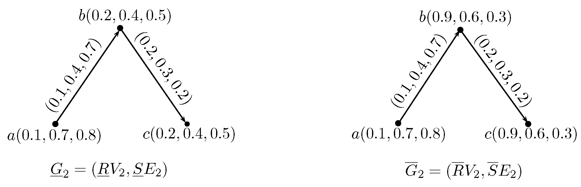
Example 1.
Let be a set and R be an equivalence relation on defined as follows:
Let be a NS on . The lower and upper approximations of are given by
Let and S be an equivalence relation on , defined as follows:
Let be a NS on and be a rough neutrosophic relation, where and are given as follows:
Thus, and are neutrosophic digraphs as shown in Figure 1.
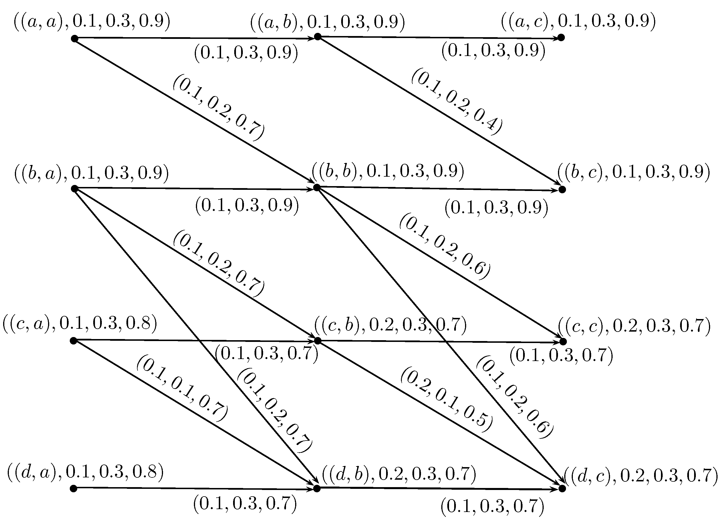
Example 2.
Let be a crisp set and R be an equivalence relation on defined as follows:
Let be a NS on and be a rough NS, where and are given as follows:
Let and S be an equivalence relation on defined as follows:
Let be a NS on ; then by definition we have
Thus, and are neutrosophic digraphs as shown in Figure 2.
Definition 5.
Let and be two rough neutrosophic digraphs on a set . Then the lexicographic product of and is a rough neutrosophic digraph , where and are neutrosophic digraphs, respectively, such that
Example 3.
Theorem 1.
The lexicographic product of two rough neutrosophic digraphs is a rough neutrosophic digraph.
Proof.
Let and be two rough neutrosophic digraphs. Let be the lexicographic product of and , where and . To prove that is a rough neutrosophic digraph, it is enough to show that and are neutrosophic relations on and , respectively. First, we show that is a neutrosophic relation on .
If , then
If , then
Thus, from the above, it is clear that is a neutrosophic relation on .
Similarly, we can show that is a neutrosophic relation on . Hence, is a rough neutrosophic digraph. ☐
Definition 6.
The strong product of two rough neutrosophic digraphs and is a rough neutrosophic digraph , where and are neutrosophic digraphs, respectively, such that
Example 4.
Theorem 2.
The strong product of two rough neutrosophic digraphs is a rough neutrosophic digraph.
Proof.
Let and be two rough neutrosophic digraphs. Let be the strong product of and , where and . To prove that is a rough neutrosophic digraph, it is enough to show that and are neutrosophic relations on and , respectively. First, we show that is a neutrosophic relation on .
If , then
If , then
If , then
Thus, from the above, it is clear that is a neutrosophic relation on .
Similarly, we can show that is a neutrosophic relation on . Hence, is a rough neutrosophic digraph. ☐
Definition 7.
Let and be two rough neutrosophic digraphs on a set . Then the rejection of and is a rough neutrosophic digraph , where and are neutrosophic digraphs, respectively, such that
Example 5.
Theorem 3.
The rejection of two rough neutrosophic digraphs is a rough neutrosophic digraph.
Proof.
Let and be two rough neutrosophic digraphs. Let be the rejection of and , where and . To prove that is a rough neutrosophic digraph, it is enough to show that and are neutrosophic relations on and , respectively. First, we show that is a neutrosophic relation on .
If , then
If , then
If , then
Thus, from the above, it is clear that is a neutrosophic relation on .
Similarly, we can show that is a neutrosophic relation on . Hence, is a rough neutrosophic digraph. ☐
Definition 8.
The tensor product of two rough neutrosophic digraphs and is a rough neutrosophic digraph , where and are neutrosophic digraphs, respectively, such that
Example 6.
Theorem 4.
The tensor product of two rough neutrosophic digraphs is a rough neutrosophic digraph.
Proof.
Let and be two rough neutrosophic digraphs. Let be the tensor product of and , where and . To prove that is a rough neutrosophic digraph, it is enough to show that and are neutrosophic relations on and , respectively. First, we show that is a neutrosophic relation on .
If , then
Thus, from the above, it is clear that is a neutrosophic relation on .
Similarly, we can show that is a neutrosophic relation on . Hence, is a rough neutrosophic digraph. ☐
Remark 1.
Hybrid-model rough neutrosophic digraphs are generalization of fuzzy digraphs and can be used to represent the relations and flows between data. Rough neutrosophic digraphs can be incrementally modified by deleting or adding elements, or they can be built by combining multiple rough neutrosophic digraphs using rough neutrosophic operations. Our proposed operations are methods of construction of new rough neutrosophic digraphs from old digraphs. By introducing the rough neutrosophic digraph theory, we have proposed a novel decision-making method based on rough neutrosophic information. It provides a new viewpoint for rough neutrosophic information. The given decision-making method can be used to evaluate upper and lower approximations to develop deep considerations of the problem.
3. Application
In this application, we use the concept of a rough neutrosophic digraph for decision-making in real-life problems. To obtain the optimal decision, we use the following formula:
where
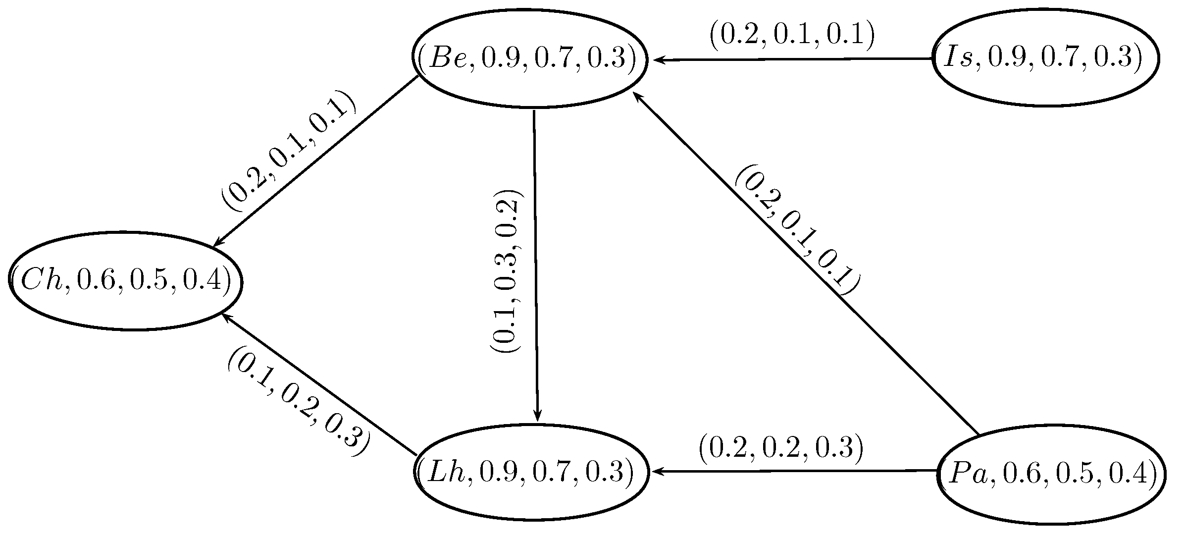
Flight planning is the process of producing a flight plan to describe a proposed aeroplane fight. Flight plans generally include basic information such as departure and arrival points, estimated time en route, and alternate airports in case of bad weather. The presented application provides alternate airports for a plane in the case of bad weather.
We suppose = {Chicago(CHI),Beijing(BJ),Lahore(LHR),Paris(PAR),Istanbul(IST)} is the set of cities under consideration and R is an equivalence relation on , where equivalence classes represent cities having the same characteristics.
We assume that a flight of Pakistan International Airways (PIA) travels to these cities. In the case of bad weather, the flight will be directed to the city with the best weather condition among the cities under consideration.
Let be a NS on that describes the characteristic of each city, and be a rough NS, where and are lower and upper approximations of V, respectively, as follows:
Let be a subset of and S be an equivalence relation on defined as follows:
where S represents the equivalence classes of “weather between different cities”. For example, the relationships (BJ,CHI),(IST,BJ) and (PAR,BJ) belong to the same equivalence class. This means that the weather between Beijing and Chicago is the same as the weather between Paris and Beijing.
Let be a NS on that describes the comparison of weathers of the cities under consideration. Let be a rough NS, where and are lower and upper approximations of E, respectively, as follows:
To find the city with the best weather condition, we use the formula that we mentioned in Equation (1).
Our decision is if , where . By direct calculations, we have
Hence the weather conditions between Istanbul and Beijing are good; can use this path in the case of a weather emergency.
We present an Algorithm 1 for the above-mentioned application. The presented algorithm can be applied to avoid lengthy calculations when dealing with a large number of objects.
| Algorithm 1: |
|
4. Conclusions
The NS model is suitable for modeling problems with uncertainty, indeterminacy and inconsistent information in which human knowledge is necessary and human evaluation is needed. Various sources of uncertainty can make it a challenge to make a reliable decision. The NS model and rough set model are used to handle uncertainty, combining these two models with another remarkable model of soft sets, giving more precise results for decision-making problems. In this paper, we have presented certain operations, including Lexicographic products and tensor products on rough neutrosophic digraphs. This research work can be extended to (1) rough bipolar neutrosophic soft graphs, (2) bipolar neutrosophic soft rough graphs, (3) interval-valued bipolar neutrosophic rough graphs, and (4) neutrosophic soft rough graphs.
Acknowledgments
The authors are very thankful to the editor and referees for their valuable comments and suggestions for improving the paper.
Author Contributions
Nabeela Ishfaq and Sidra Sayed conceived and designed the experiments; Muhammad Akram performed the experiments; Florentin Smarandache contributed reagents/materials/analysis tools.
Conflicts of Interest
The authors declare that they have no conflict of interest regarding the publication of the research article.
References
- Smarandache, F. A Unifying Field in Logics. Neutrosophy: Neutrosophic Probability, Set and Logic; America Research Press: Rehoboth, NM, USA, 1999. [Google Scholar]
- Smarandache, F. Neutrosophy: Neutrosophic Probability, Set and Logic; America Research Press: Rehoboth, NM, USA, 1998. [Google Scholar]
- Wang, H.; Smarandache, F.; Zhang, Y.; Sunderraman, R. Single-valued neutrosophic sets. Rev. Air Force Acad. 2010, 4, 410–413. [Google Scholar]
- Ye, J. Multicriteria decision-making method using the correlation coefficient under single-valued neutrosophic environment. Int. J. Gen. Syst. 2013, 42, 386–394. [Google Scholar] [CrossRef]
- Pawlak, Z. Rough sets. Int. J. Comput. Inf. Sci. 1982, 5, 341–356. [Google Scholar] [CrossRef]
- Dubois, D.; Prade, H. Rough fuzzy sets and fuzzy rough sets. Int. J. Gen. Syst. 1990, 17, 191–209. [Google Scholar] [CrossRef]
- Liu, P.; Chen, S.M. Group decision making based on Heronian aggregation operators of intuitionistic fuzzy numbers. IEEE Trans. Cybern. 2017, 47, 2514–2530. [Google Scholar] [CrossRef] [PubMed]
- Broumi, S.; Smarandache, F.; Dhar, M. Rough neutrosophic sets. Neutrosophic Sets Syst. 2014, 3, 62–67. [Google Scholar]
- Yang, H.L.; Zhang, C.L.; Guo, Z.L.; Liu, Y.L.; Liao, X. A hybrid model of single valued neutrosophic sets and rough sets: Single valued neutrosophic rough set model. Soft Comput. 2017. [Google Scholar] [CrossRef]
- Mordeson, J.N.; Peng, C.S. Operations on fuzzy graphs. Inf. Sci. 1994, 79, 159–170. [Google Scholar] [CrossRef]
- Akram, M.; Shahzadi, S. Neutrosophic soft graphs with application. J. Intell. Fuzzy Syst. 2017, 32, 841–858. [Google Scholar] [CrossRef]
- Akram, M.; Sarwar, M. Novel multiple criteria decision making methods based on bipolar neutrosophic sets and bipolar neutrosophic graphs. Ital. J. Pure Appl. Math. 2017, 38, 368–389. [Google Scholar]
- Akram, M.; Siddique, S. Neutrosophic competition graphs with applications. J. Intell. Fuzzy Syst. 2017, 33, 921–935. [Google Scholar] [CrossRef]
- Akram, M.; Sitara, M. Interval-valued neutrosophic graph structures. Punjab Univ. J. Math. 2018, 50, 113–137. [Google Scholar]
- Zafer, F.; Akram, M. A novel decision-making method based on rough fuzzy information. Int. J. Fuzzy Syst. 2017, 1–15. [Google Scholar] [CrossRef]
- Sayed, S.; Ishfaq, N.; Akram, M.; Smarandach, F. Rough neutrosophic digraphs with application. Axioms 2018, 7, 5. [Google Scholar] [CrossRef]
- Banerjee, M.; Pal, S.K. Roughness of a fuzzy set. Inf. Sci. 1996, 93, 235–246. [Google Scholar] [CrossRef]
- Bao, Y.L.; Yang, H.L. On single valued neutrosophic refined rough set model and its application. J. Intell. Fuzzy Syst. 2017, 33, 1235–1248. [Google Scholar] [CrossRef]
- Ye, J. Improved correlation coefficients of single valued neutrosophic sets and interval neutrosophic sets for multiple attribute decision making. J. Intell. Fuzzy Syst. 2014, 27, 2453–2462. [Google Scholar]
- Zadeh, L.A. Fuzzy sets. Inf. Control 1965, 8, 338–353. [Google Scholar] [CrossRef]
- Zhang, X.; Dai, J.; Yu, Y. On the union and intersection operations of rough sets based on various approximation spaces. Inf. Sci. 2015, 292, 214–229. [Google Scholar] [CrossRef]
Figure 1.
Rough neutrosophic digraph .
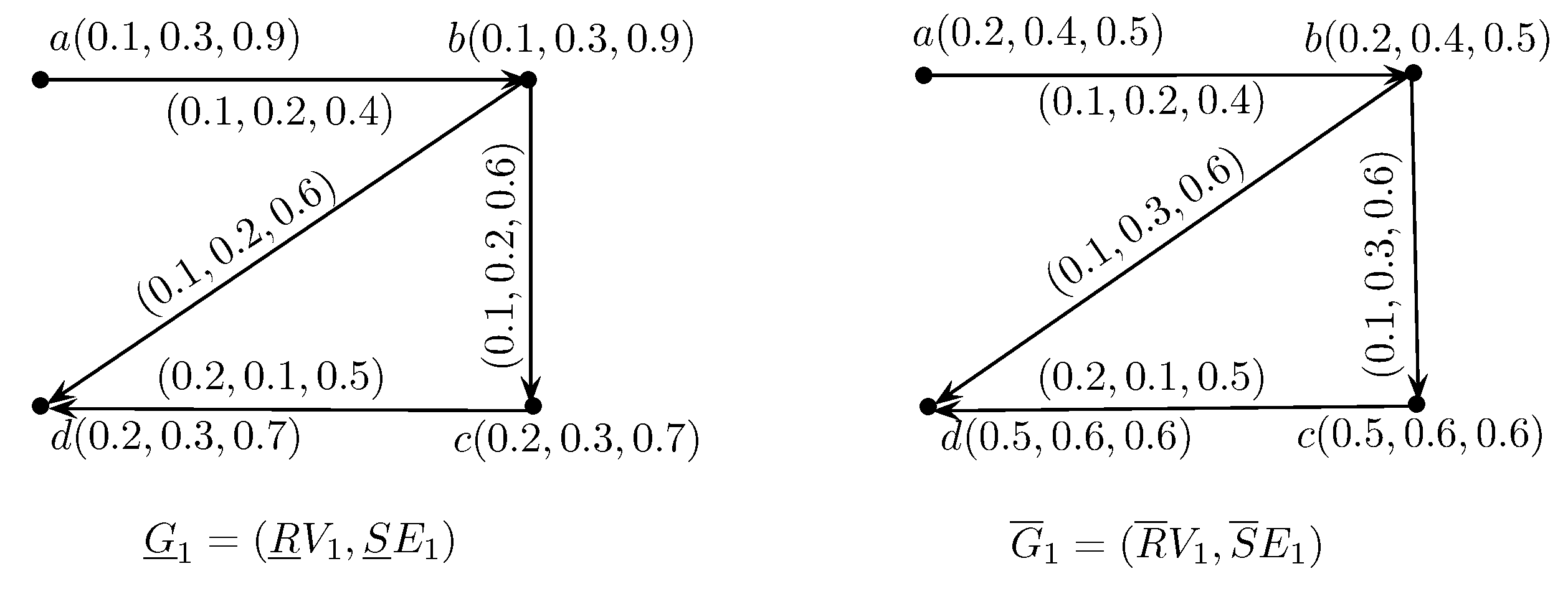
Figure 2.
Rough neutrosophic digraph .

Figure 3.
Neutrosophic digraph .

Figure 4.
Neutrosophic digraph .
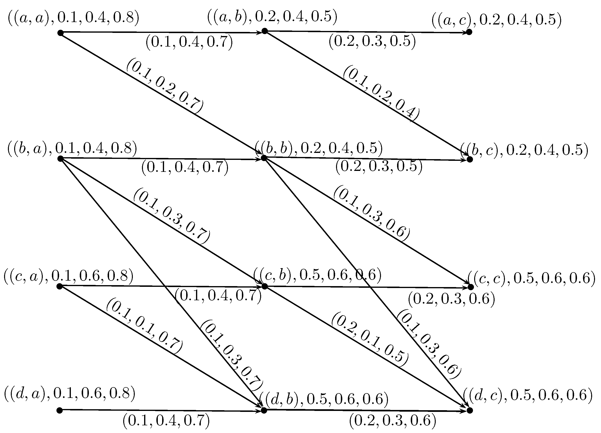
Figure 5.
Neutrosophic digraph .
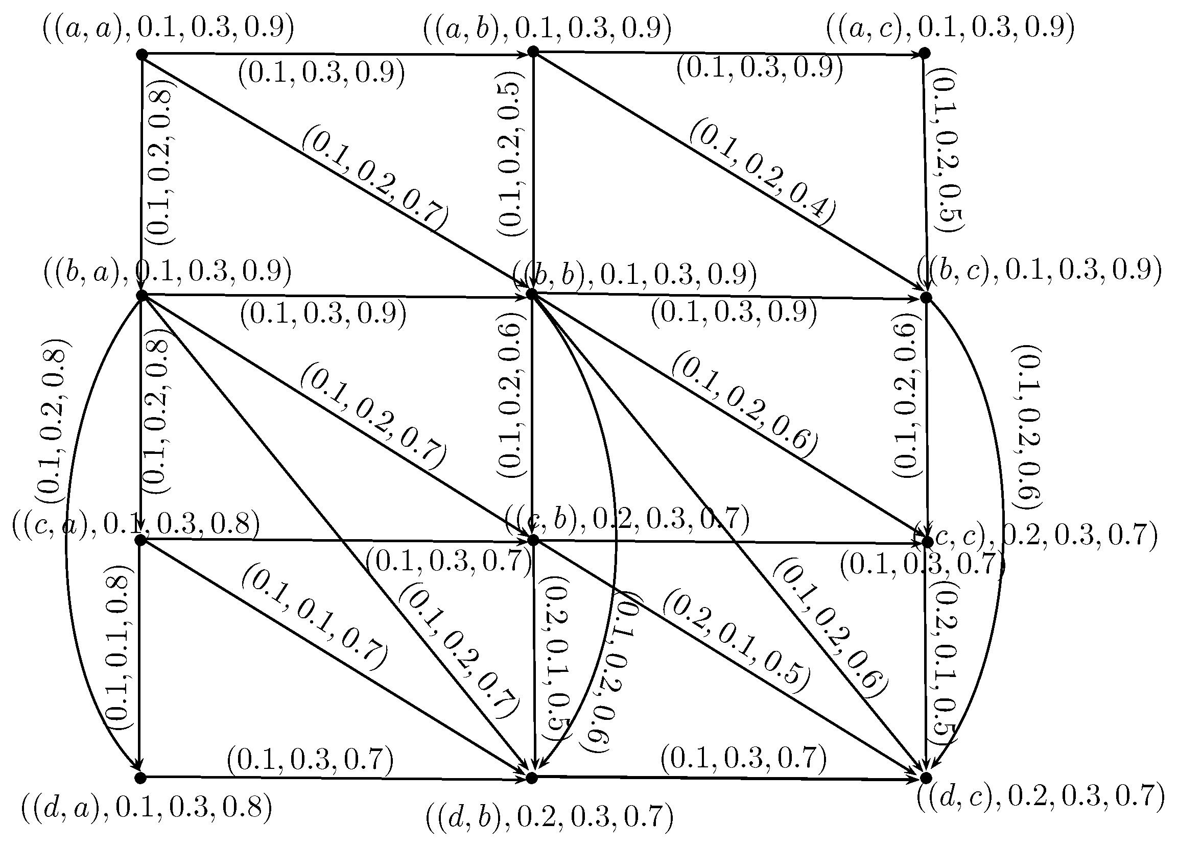
Figure 6.
Neutrosophic digraph .
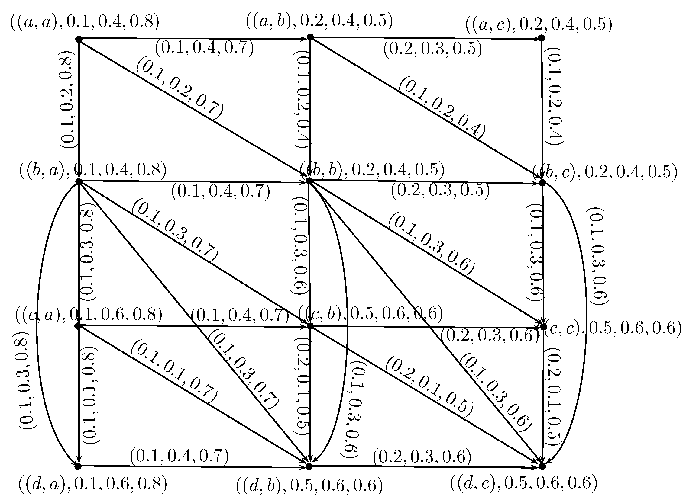
Figure 7.
Rough neutrosophic digraph .
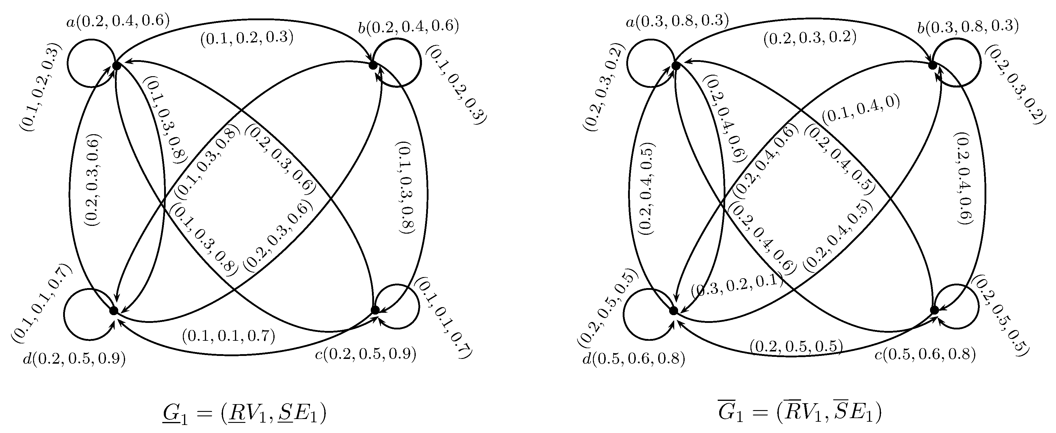
Figure 8.
Rough neutrosophic digraph .
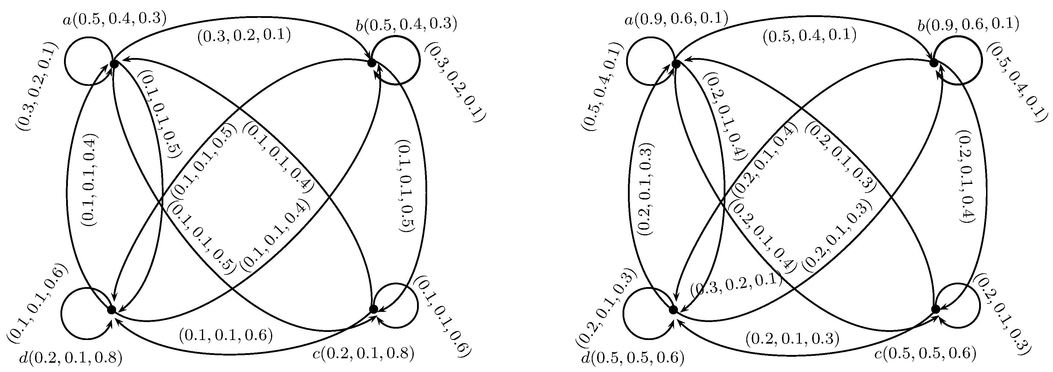
Figure 9.
Neutrosophic digraph .

Figure 10.
Neutrosophic digraph .
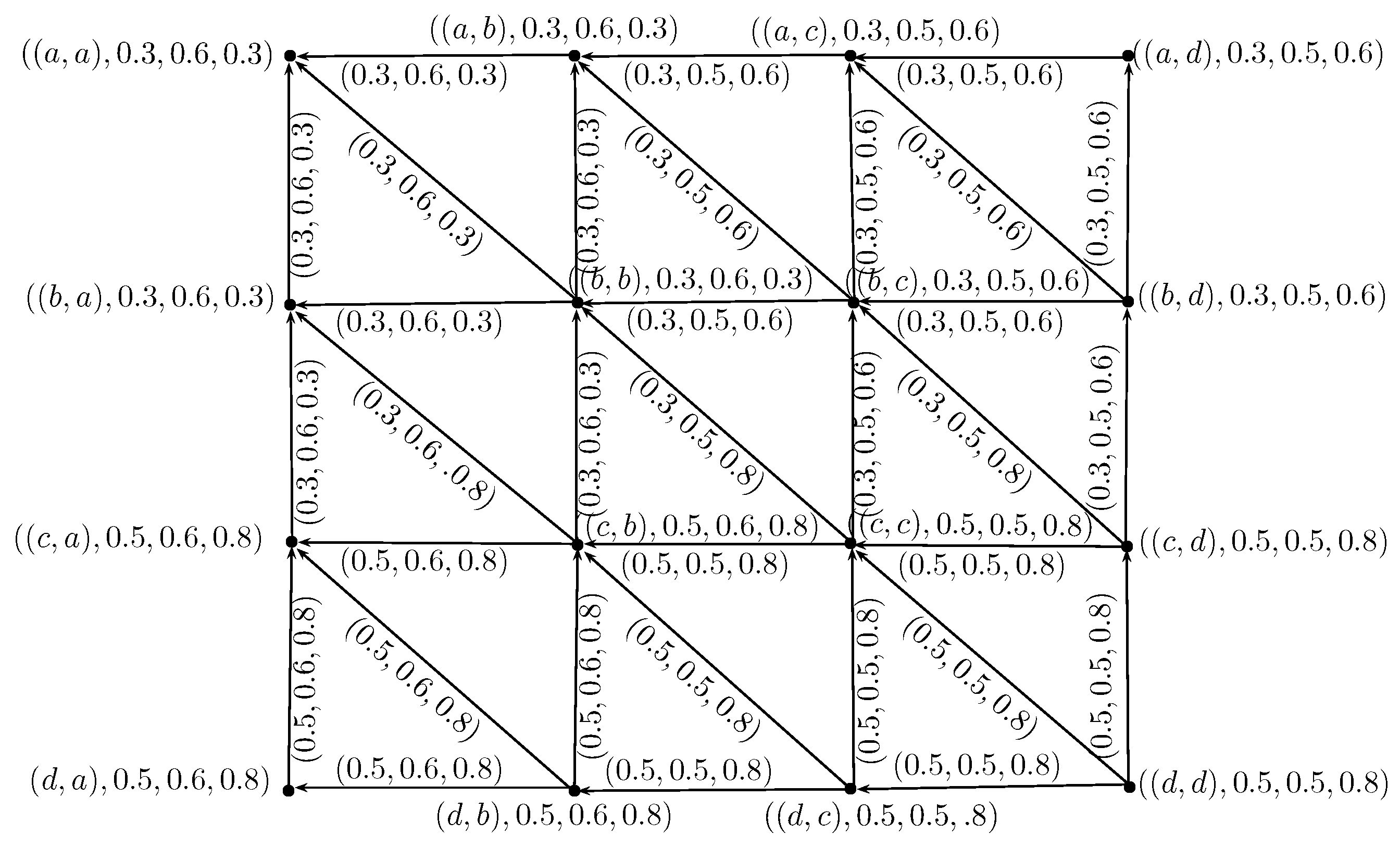
Figure 11.
Rough neutrosophic digraph .
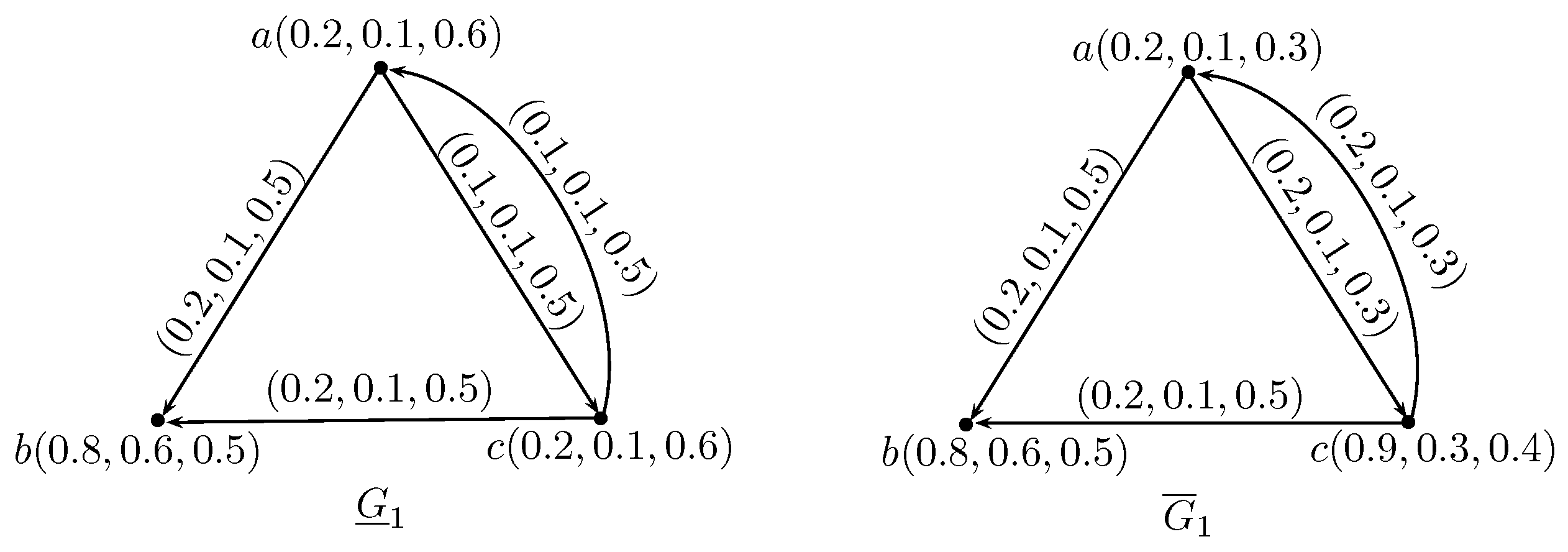
Figure 12.
Rough neutrosophic digraph .

Figure 13.
Neutrosophic digraph .
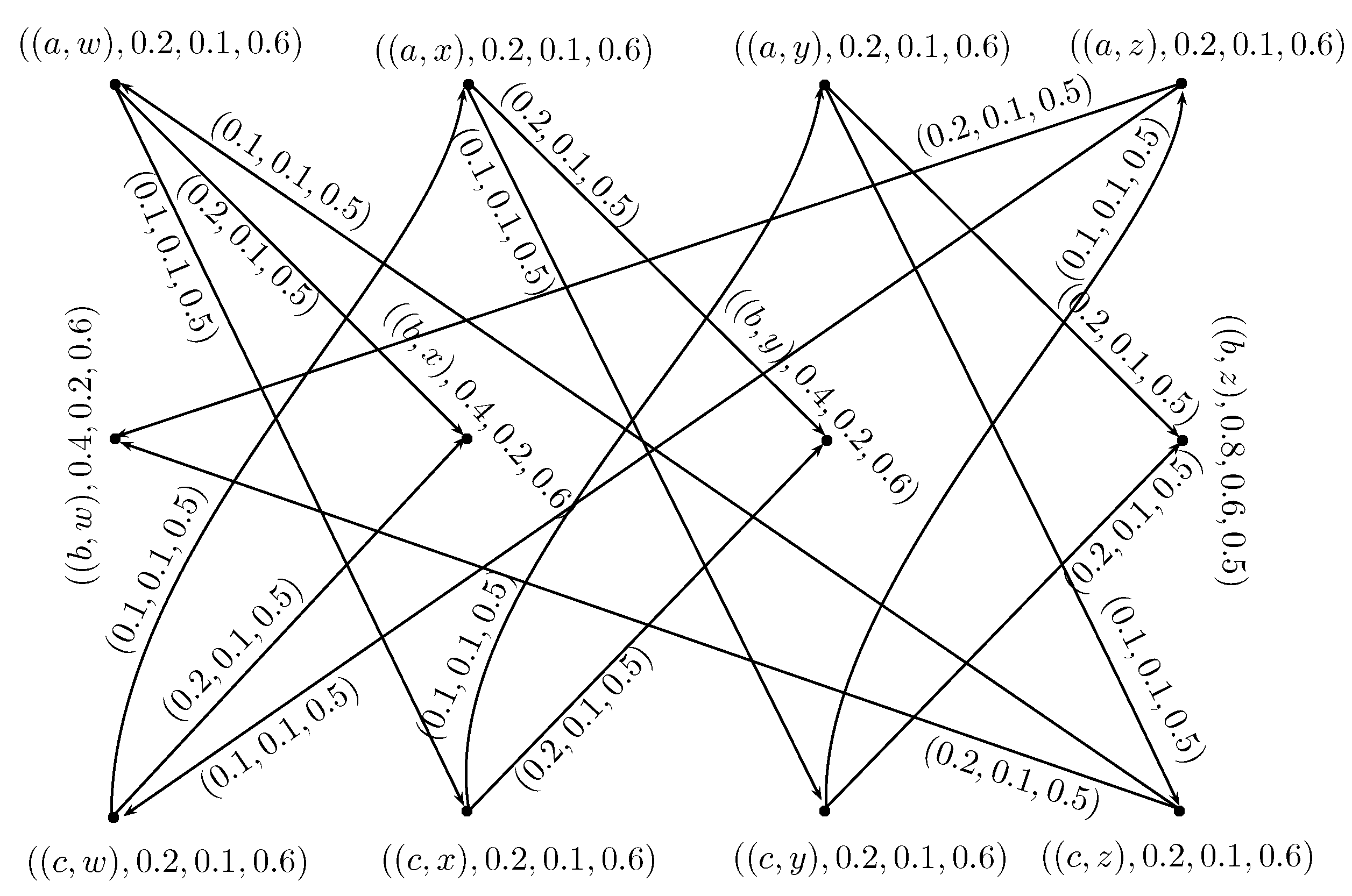
Figure 14.
Neutrosophic digraph .
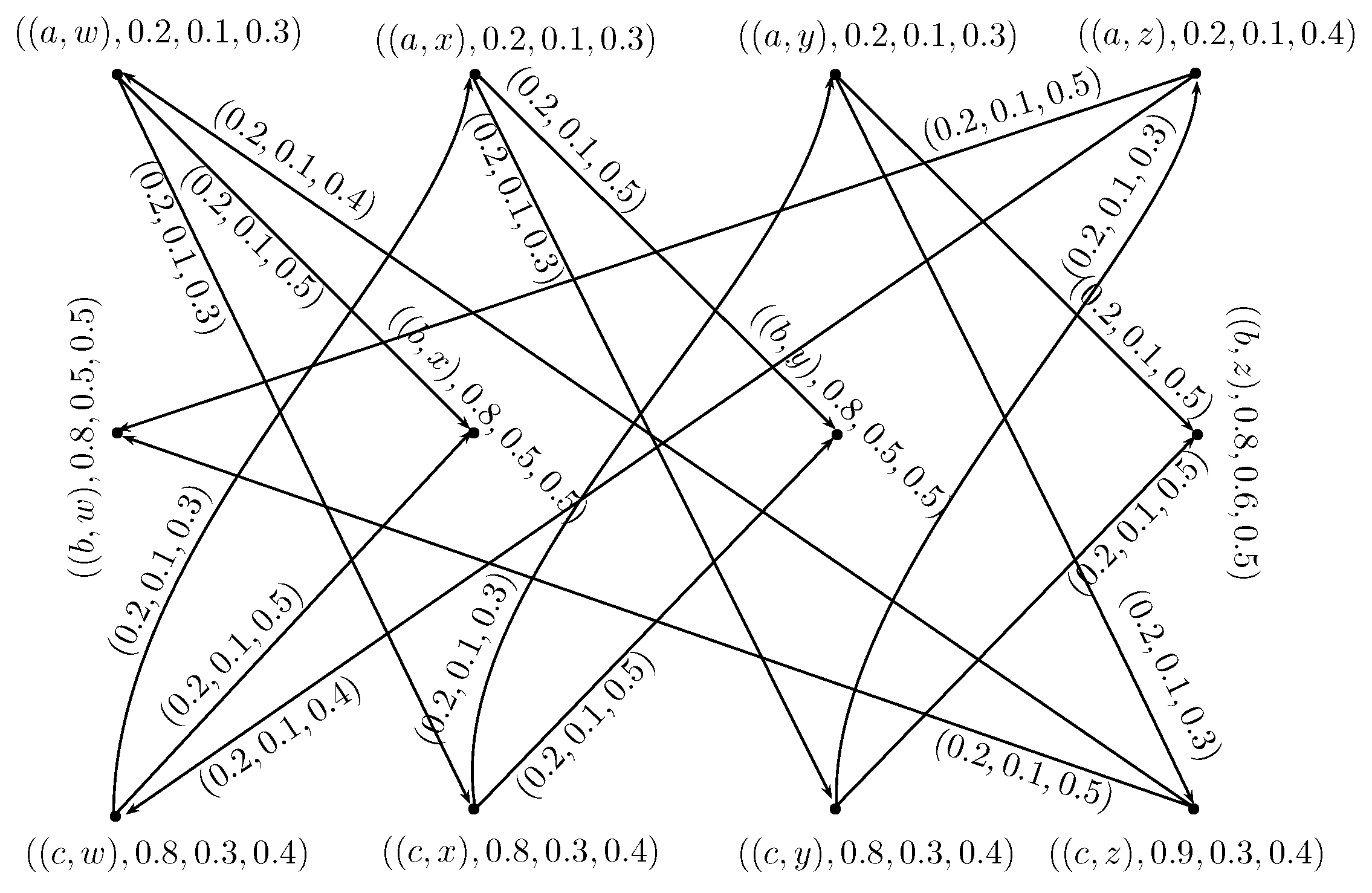
Figure 15.
Neutrosophic digraph .

Figure 16.
Neutrosophic digraph .

© 2018 by the authors. Licensee MDPI, Basel, Switzerland. This article is an open access article distributed under the terms and conditions of the Creative Commons Attribution (CC BY) license (http://creativecommons.org/licenses/by/4.0/).
Share and Cite
MDPI and ACS Style
Ishfaq, N.; Sayed, S.; Akram, M.; Smarandache, F. Notions of Rough Neutrosophic Digraphs. Mathematics 2018, 6, 18. https://doi.org/10.3390/math6020018
AMA Style
Ishfaq N, Sayed S, Akram M, Smarandache F. Notions of Rough Neutrosophic Digraphs. Mathematics. 2018; 6(2):18. https://doi.org/10.3390/math6020018
Chicago/Turabian StyleIshfaq, Nabeela, Sidra Sayed, Muhammad Akram, and Florentin Smarandache. 2018. "Notions of Rough Neutrosophic Digraphs" Mathematics 6, no. 2: 18. https://doi.org/10.3390/math6020018
Note that from the first issue of 2016, this journal uses article numbers instead of page numbers. See further details here.