Advanced Expected Tail Loss Measurement and Quantification for the Moroccan All Shares Index Portfolio

Abstract

In this paper, we have analyzed and tested the Expected Tail Loss (ETL) approach for the Value at Risk (VaR) on the Moroccan stock market portfolio. We have compared the results with the general approaches for the standard VaR, which has been the most suitable method for Moroccan stock investors up to now. These methods calculate the maximum loss that a portfolio is likely to experience over a given time span. Our work advances those modeling methods with supplementation by inputs from the ETL approach for application to the Moroccan stock market portfolio—the Moroccan All Shares Index (MASI). We calculate these indicators using several methods, according to an easy and fast implementation with a high-level probability and with accommodation for extreme risks; this is in order to numerically simulate and study their behavior to better understand investment opportunities and, thus, form a clear view of the Moroccan financial landscape.

1. Introduction

Extended financial risk management is the immediate solution to which researchers, economists, and financial managers have turned since the last crisis. During extreme events, they aim to better understand the financial market by minimizing the potential losses of portfolio assets. In order to improve current risk indicators, they have focused their work on studying the distribution tail of these losses.

The quantification of risk for good management was introduced by H. Markowitz [1] in his seminal article, through his famous Mean–Variance model based on the principle of diversification. With its assumption that the risk of a portfolio can be properly mitigated by volatility measured by the variance of its profitability, this model has often been the target of severe criticism.

Another model, the Sharp’s Capital Asset Pricing Model (CAPM) [2], also looked at the problem of risk quantification. As a monofactorial model, the CAPM, which presents its famous Beta coefficient as a portfolio risk measure, also shows certain shortcomings—in particular, the instability of this coefficient, and the almost absolute difficulties of verifying the hypotheses on which the model itself is based.

The weakness and inadequacies of these models, which are mainly related to the distribution of risk factors, the arrival and development of derivatives, the increase in volatility, and the complexity of financial markets, have prompted financial managers to implement a global and synthetic risk measure that can incorporate any nonlinearity into the distribution of returns on financial assets, while focusing on the potential value to be lost rather than on changes in the market value of financial assets.

Thus, Value at Risk (VaR) and Expected Tail Loss (ETL) are certainly the most commonly used risk measures in the financial industry to quantify the amount at risk in a portfolio [3]. Central to risk management, VaR is a very simple concept, which, for a given portfolio, a given time horizon, and a threshold p, gives the level of loss which should only be exceeded by (1 − p)%. It is a particular way to summarize and describe the magnitude of probable losses in a portfolio, making it useful for measuring and comparing the risks of different market portfolios and comparing the risk of the same portfolio at different times. Notwithstanding its qualities and ease of implementation, it has a number of shortcomings—in particular, those relating to the nonverification of the principle of diversification (subadditivity) and the nonconsideration of extreme events. These negative points are improved upon by the extension of the VaR: the ETL.

This work will focus on the analysis of indicators used to measure a financial instruments portfolio’s market risk. We will start by introducing risk measurement models. We introduce VaR and its extension, ETL.

We calculate these two indicators using several methods for a portfolio of equities (the representative portfolio of the Moroccan stock market, the Moroccan All Share Index (MASI) in order to numerically simulate these indicators and study their behavior to better understand investment opportunities and, thus, have a clear view of the Moroccan financial landscape.

The article will be organized in three sections. First, we will present the VaR model and three calculation approaches (historical, parametric, and Monte Carlo). Then we will present the ETL model as a complementary and alternative measure to VaR; ETL is also considered a more concise and efficient measure than VaR in terms of estimating extreme events. Finally, the main work will be the practical implementation of those methods on the MASI, followed by general conclusions of our work.

2. Value at Risk and Its Complements

VaR is a concept that has established itself as the benchmark measure of risk—market risk, to be precise. The VaR of a financial security is a number that is able to summarize the risk incurred in that security. This concept first emerged in the insurance industry. Bankers Trust imported it in the late 1980s into financial markets in the United States, but it was mainly JP Morgan Bank that popularized this concept in 1993 by means of its Risk Metrics system [4].

VaR is a financial asset’s probable loss amount, usually for a portfolio or portfolio set. It presents the loss that a portfolio will incur as a result of adverse changes in market prices.

Generally, it is defined as the maximum loss that with reasonably certainty will not be exceeded at a given probability if the current portfolio is maintained unchanged over a certain period of time [5]. For example, for a 95% probability and a 1 day time horizon, a VaR that displays 1 million MAD (Moroccan Dirham) means that the loss that the instrument may suffer will not exceed 1 million MAD on the next day in 95% of cases.

2.1. Value at Risk Parameters

VaR is based on three essential parameters for its modeling:

-

The level of confidence;

-

The horizon;

-

The distribution of risk factors.

The confidence level is an important variant in VaR modelling. It is often determined by an external regulator (as in the case of banks). Under the Basel Accord, banks use internal VaR models. The materiality level is set at 1%. In general, and in the absence of regulation, this parameter will depend on the investor’s attitude to risk. The higher the risk aversion, the smaller the alpha, and the higher the confidence level will be.

The horizon represents the period over which the instrument held will undergo market fluctuations and give rise to profit or loss. Generally, the choice of this parameter depends on both the liquidity of the market and the nature of the portfolio management; the horizon must correspond to the duration necessary to ensure the liquidity of the instrument, so its composition must be unchanged over this horizon.

Yield distribution is the most difficult parameter to determine. It is determined according to the risk factors on the fixed horizon. In most cases this distribution is assumed to be normal, but risk factors rarely verify this assumption. Empirically, two problems govern the financial time series: The first is the nonstationarity of the series. The second is the leptokurtic character of the distribution which corresponds to very thick tails compared with those considered by the reference law (normal law); this can result in the under- or overestimation of VaR and, thus, more risk assumed by the investor.

These parameters are essential for VaR estimation. This can lead to an under- or overestimation of the true value displayed by the VaR; the representativeness can be modeled as follows [6]:

VaR is defined as the loss in terms of the current value of the portfolio, which one is sure not to exceed with a predetermined probability due to market movements. Mathematically, VaR consists of finding the quintile $\mathsf{\alpha }$, denoted ${\mathrm{x}}_{\mathrm{t},\mathsf{\alpha }}$, of the distribution of risk factors. Thus, we can write [5]

$$\mathrm{P}\left({\mathrm{P}}_{\mathrm{t}+\mathrm{h}}-{\mathrm{P}}_{\mathrm{t}}<{\mathrm{x}}_{\mathrm{t},\mathsf{\alpha }}\right)=\mathsf{\alpha }$$

(1)

$${\mathrm{VaR}}_{\mathrm{t},\mathsf{\alpha }}=-{\mathrm{x}}_{\mathrm{t},\mathsf{\alpha }}$$

(2)

where ${\mathrm{P}}_{\mathrm{t}}$ is the price of the security at date t and $\mathsf{\alpha }$ is the confidence threshold.

A VaR estimated from the distribution of profits and losses (P&L) is expressed in a value (an amount x) which requires us to pay attention to the interpretation of the results because a $\mathrm{VaR}=100$ $\mathrm{MAD}$ for a $1000 \mathrm{MAD}$ value portfolio is not the same as a $\mathrm{VaR}=100$ for a $1 \mathrm{MMAD}$ value portfolio. For this reason, it is preferable to work with a yield distribution rather than P&L, since yields are measured in relative terms and can be comparable over long periods of time, especially since VaR can be presented as a percentage of the overall value of the portfolio. Thus, if we define a random variable X linked to portfolio returns on a given date, we will have

$${\mathrm{X}}_{\mathrm{t}}=\frac{{\mathrm{P}}_{\mathrm{t}+\mathrm{h}}-{\mathrm{P}}_{\mathrm{t}}}{{\mathrm{P}}_{\mathrm{t}}} .$$

(3)

Thus, the new VaR definition will be in terms of the percentage as

$$\mathrm{P}\left({\mathrm{X}}_{\mathrm{t}}<{\mathrm{x}}_{\mathrm{t},\mathsf{\alpha }}\right)=\mathrm{P}\left(\frac{{\mathrm{P}}_{\mathrm{t}+\mathrm{h}}-{\mathrm{P}}_{\mathrm{t}}}{{\mathrm{P}}_{\mathrm{t}}}<{\mathrm{x}}_{\mathrm{t},\mathsf{\alpha }}\right)=\mathsf{\alpha },$$

(4)

$${\mathrm{VaR}}_{\mathrm{t},\mathsf{\alpha }}=-{\mathrm{x}}_{\mathrm{t},\mathsf{\alpha }}.$$

(5)

As the value of the portfolio ${\mathrm{P}}_{\mathrm{t}}$ is known, the VaR amount can be obtained by multiplying the VaR by the percentage ${\mathrm{P}}_{\mathrm{t}}$:

$${\mathrm{VaR}}_{\mathrm{t},\mathsf{\alpha }}=-{\mathrm{x}}_{\mathrm{t},\mathsf{\alpha }}\ast {\mathrm{P}}_{\mathrm{t}}.$$

(6)

2.2. Risk Measurement Calculation Methods

VaR modeling is essentially based on three approaches: the historical method, parametric method, and the Monte Carlo simulation method. Each of these methods will be applied to the MASI portfolio.

2.2.1. Historical Value at Risk

Based essentially on the instrument risk factor variation history (prices, interest rates, etc.), the historical method (also called the nonparametric method) is the simplest and the most widely used. This is due to its ease of implementation based on the hypothesis of the stationarity of the various risk factors. The historical VaR model assumes that the distribution of historically simulated returns will be identical to the distribution of future returns [6].

The principle of the method is simple: based on a portfolio price history sample, risk factors are determined. As an example, for a stock portfolio, a historical yields sample is determined to identify the risk factors that are no more than the variation in the price of the securities making up the portfolio. Once this is done, the portfolio returns are sorted (in ascending order) and the fractile linked to the fixed probability is determined. If we consider a 95% confidence level and have a sample of 100 observations of historical performance, the VaR is the 50th largest loss. If the resulting number is not an integer, linear interpolation is used.

2.2.2. Parametric Value at Risk

The parametric method is based on a number of assumptions: the temporal independence of changes in the value of the portfolio, the normality, and the linearity of risk factors [3].

Assuming the normality of risk factors we have ${\mathrm{X}}_{\mathrm{t}}~\mathrm{N}\left(\mathsf{\mu },{\mathsf{\sigma }}^2\right)$ where ${\mathrm{X}}_{\mathrm{t}}$ is the portfolio yield at time t.

$$\mathrm{P}\left({\mathrm{X}}_{\mathrm{t}}<{\mathrm{x}}_{\mathrm{t},\mathsf{\alpha }}\right)=\mathsf{\alpha }$$

(7)

In order to extract the quantile related to our supposed normal distribution, we center and reduce:

$$\mathrm{P}\left(\frac{{\mathrm{X}}_{\mathrm{t}}-\mathsf{\mu }}{\mathsf{\sigma }}<\frac{{\mathrm{x}}_{\mathrm{t},\mathsf{\alpha }}-\mathsf{\mu }}{\mathsf{\sigma }}\right)=\mathrm{P}\left(\mathrm{Z}<\frac{{\mathrm{x}}_{\mathrm{t},\mathsf{\alpha }}-\mathsf{\mu }}{\mathsf{\sigma }}\right)=\mathsf{\alpha }$$

(8)

with $\mathrm{Z}~\mathrm{N}\left(0,1\right)$.

Furthermore, it is known that by definition that

$$\mathrm{P}\left(\mathrm{Z}<\mathsf{\Phi }\left(\mathsf{\alpha }\right)\right)=\mathsf{\alpha },$$

(9)

$$\mathrm{P}\left(\mathrm{Z}<\mathsf{\Phi }\left(\mathsf{\alpha }\right)\right)=\mathsf{\alpha },$$

(10)

$${\mathrm{x}}_{\mathrm{t},\mathsf{\alpha }}={\mathsf{\Phi }}^{-1}\left(\mathsf{\alpha }\right)\ast \mathsf{\sigma }+\mathsf{\mu }.$$

(11)

Or, according to Equation (2), we have

$${\mathrm{VaR}}_{\mathrm{t},\mathsf{\alpha }}=-{\mathrm{x}}_{\mathrm{t},\mathsf{\alpha }}.$$

(12)

Given that

$${\mathsf{\Phi }}^{-1}\left(\mathsf{\alpha }\right)=-{\mathsf{\Phi }}^{-1}\left(1-\mathsf{\alpha }\right)$$

where $\mathsf{\Phi }$ is the distribution function of the normal law, we have

$${\mathrm{VaR}}_{\mathrm{t},\mathsf{\alpha }}=-\left(-{\mathsf{\Phi }}^{-1}\left(1-\mathsf{\alpha }\right)\ast \mathsf{\sigma }+\mathsf{\mu }\right),$$

(13)

$${\mathrm{VaR}}_{\mathrm{t},\mathsf{\alpha }}={\mathsf{\Phi }}^{-1}\left(1-\mathsf{\alpha }\right)\ast \mathsf{\sigma }-\mathsf{\mu }.$$

(14)

Thus, for a series of yields ${\mathrm{R}}_{\mathrm{t}}$ with $t = 1,2,\dots n$, we obtain

$$\mathsf{\mu }=\mathrm{E}\left(\mathrm{R}\right) \mathrm{et} \mathsf{\sigma }=\mathsf{\sigma }\left(\mathrm{R}\right),$$

(15)

$$\mathrm{VaR}={\mathrm{Z}}_{1-\mathsf{\alpha }}\ast \mathsf{\sigma }\left(\mathrm{R}\right)-\mathrm{E}\left(\mathrm{R}\right).$$

(16)

Note, however, that for this method it is possible to distinguish between absolute VaR and relative VaR, as

$$\mathrm{Absolute}\mathrm{VaR}=\mathrm{Relative}\mathrm{VaR}-\mathrm{Expected}\mathrm{average}\mathrm{portfolio}\mathrm{yield}.$$

2.2.3. The Value at Risk Monte Carlo

Unlike the other two methods, which were based on historical data for the VaR calculation, the Monte Carlo method is based on the simulation principle. In this case, the quantile extraction will not be done based on the actual history of the risk factors, but on a simulated history using the Monte Carlo simulation method. This method is similar in fractile determination to the historical method.

The difference lies in the calculation basis. The first method is based on simulated data, while the latter method is based on real history. The Monte Carlo method is particularly suitable for optional instruments where the distribution law is difficult to model [3].

The Monte Carlo simulation principle can be summed up in four essential steps:

Step 1: Generation of random vectors resulting from the chosen law.

This step consists of generating k independent random variables that we will represent by the vector $\mathrm{Z}=\left(\mathrm{Z}1,\mathrm{Z}2,\dots ,\mathrm{Zk}\right)$. Each generated Z-line vector is called a simulated scenario.

Step 2: Decomposition of Cholesky.

Any symmetrical and defined positive D-matrix can be factorized as $\mathrm{D}={\mathrm{AA}}^{\mathrm{T}}$ where A is a square, lower-triangular matrix.

Matrix A is not unique. Thus, several factorizations of a given matrix D are possible. These factorizations are known as Cholesky factorizations. When D is a positive defined matrix, matrix A is unique.

The covariance–variance matrix $\mathrm{\Sigma }$ has the same properties as the matrix D. We then undergo a Cholesky decomposition in the form $\mathrm{\Sigma }={\mathrm{AA}}^{\mathrm{T}}$, with

$$A=\left(\begin{array}{ccc}{a}_{1,1}& a_{2,1}& \begin{array}{cc}\dots & a_{n,1}\end{array}\\ a_{2,1}& a_{2,2}& \begin{array}{cc}\dots & a_{2,n}\end{array}\\ \begin{array}{c}⋮\\ a_{n,1}\end{array}& \begin{array}{c}⋮\\ \dots \end{array}& \begin{array}{c}\begin{array}{cc}\ddots & ⋮\end{array}\\ \begin{array}{cc}\dots & a_{n,n}\end{array}\end{array}\end{array}\right).$$

(17)

The coefficients of matrix A are given by the following equations:

$$a_{ij}=\{\begin{array}{c} 0 for j<i\\ \sqrt{{\sigma }_{ii}-{\displaystyle {\displaystyle \sum }_{k=1}^{i-1}}{a}_{jk}^2} for j=i\\ \frac{1}{a_{ii}}{\sigma }_{ij}-{\displaystyle {\displaystyle \sum }_{k=1}^{i-1}}{a}_{ik}-a_{jk} for j>i\end{array}$$

(18)

where

• ${\sigma }_{ii}:$ Variance;
• ${\sigma }_{ij}:$ Covariance between the security i and the security j.

Step 3: Calculate the return scenarios.

Let $\mathrm{r}=({\mathrm{r}}_1,{\mathrm{r}}_2,\dots {\mathrm{r}}_{\mathrm{k}}$) be the vector of simulated returns over h days. Each simulated vector represents a scenario of returns. These scenarios are calculated as follows: We try to generate random vectors derived from the chosen law from the Z random vectors generated at the level of the first stage (simulated scenarios). This transformation is done as follows:

$$\mathrm{r}={\mathrm{AZ}}^{\mathrm{t}}+\mathsf{\mu }$$

(19)

where

• $\mathrm{A}:$ The Cholesky factorization matrix of the variance–covariance matrix $\mathrm{\Sigma }$;
• ${\mathrm{Z}}^{\mathrm{t}}:$ Transposed random vectors;
• $\mathsf{\mu }:$ Vector of simulated scenario averages.

Finally, the vector of returns r must be multiplied by the corresponding weights in order to obtain the history of the portfolio’s returns.

Step 4: Calculate the VaR.

From the calculated history, it is enough to take the order quantile $\mathsf{\alpha }$ of this distribution. This quantile corresponds to the VaR value at horizon $\mathrm{T}$ and the threshold $\mathsf{\alpha }\%$.

It can be concluded that the Monte Carlo method is similar to the historical simulation except that Monte Carlo VaR uses simulated factors.

2.3. Value at Risk Complementary Risk Measures

The properties to be verified for a consistent risk measure [5] are mainly monotony, translation invariance, homogeneity, and subadditivity.

In the case of VaR, the analysis of all these characteristics makes it possible to assert that it does not verify the axiom of subadditivity, which is a very important property on which the principle of diversification is based. The VaR of each individual security does not take into account the correlation effect between the securities, which is one of the most important principles for reducing risk.

2.3.1. Subadditivity Remedied by PVaR

The principle of diversification is one of the most important phenomena in modern finance. It allows risk reduction based on the correlation effect between securities. In principle, financial securities do not all move in the same direction at any given time; some of them move in a positive direction and others move in the opposite direction, which is why a portfolio composed of securities with different correlations allows for the easing of shocks linked to price fluctuations [7].

However, we are intrigued by a question: if the diversification principle cannot be applied to VaR, why would the investor adopt it as a substitute for other measures?

Based on Euler’s theorem, a decomposition method will be proposed for VaR in order to define the portion of the VaR of the portfolio allocated to each asset, so that the overall VaR of the portfolio will be less than or equal to the sum of the VaR of each security in the portfolio [8].

The VaR of each security in this case is called the Partial VaR, denoted PVaR. It is defined by the following formula:

$$\mathrm{PVaR}=\frac{\partial \mathrm{VaR}\left(\omega \right)}{\partial {\omega }_i}\ast {\omega }_i$$

(20)

where

• $\mathrm{VaR}\left(\omega \right):\mathrm{the}\mathrm{Global}\mathrm{portfolio}\mathrm{VaR};$
• ${\omega }_i:\mathrm{the}\mathrm{weight}\mathrm{of}\mathrm{security}\mathrm{i}\mathrm{making}\mathrm{up}\mathrm{the}\mathrm{portfolio}.$

VaR is then the sum of the N-many PVaRs.

Thus, we write

$${\mathrm{VaR}}_{\mathsf{\alpha }}={\displaystyle \sum }_{i=1}^N{\mathrm{PVaR}}_{\mathsf{\alpha }}.$$

(21)

Demonstration of the PVaR: To try to extract the formula of the PVaR, we will refer to Euler’s law (or Euler’s theorem).

Theorem 1.

A function of several variables f: ℝn → ℝm differentiable at any point is (positively) homogeneous of degree k if, and only if, the following equation, called the Euler identity, is verified:

$$\forall \left(x_1\dots \dots x_n\right)\in R^n,{\displaystyle \sum }_{i=1}^n{x}_i\frac{\partial f}{\partial x_i}\left(x\right)=kf\left(x\right).$$

(22)

This theorem will be applied to the VaR of a portfolio in order to obtain the PVaR of each security. We will begin by stating that the value of the portfolio is $kw$ where $k>0$ and $\omega$ is the weighting vector of the securities making up our portfolio.

Let $\omega =\left({\omega }_1,{\omega }_2,\dots \dots ,{\omega }_n\right)$ be the weighting vector of the assets making up the portfolio, and let $\sigma \left(\omega \right) \mathrm{and}\mathrm{VaR}\left(\omega \right)$, respectively, be the volatility and VaR of the portfolio, which depend on the weight of the securities. All weightings in the portfolio will be multiplied by the same ratio $k>0$; that is, the new vector considered will be $k\omega =\left(k{\omega }_1,k{\omega }_2,\dots \dots ,k{\omega }_n\right)$, and the standard deviation and VaR of the portfolio will, respectively, be $\sigma \left(k\omega \right)$ and $\mathrm{VaR}\left(k\omega \right)$. Since the standard deviation and VaR are two homogeneous risk measures, we can write

$$\sigma \left(k\omega \right)=k\sigma \left(\omega \right),$$

(23)

$$\mathrm{VaR}\left(k\omega \right)=k\mathrm{VaR}\left(w\right).$$

(24)

Thus, increasing the size of a portfolio by a positive k-factor simply multiplies the risk by the same k-factor.

Since the standard deviation and the VaR are two differentiable and homogeneous measures, we then proceed to the Euler theorem verification; for this, the two parts of each equation are differentiated beside k. This derivative provides an estimation of the effect of an increase in all the positions in our portfolio on the VaR and the standard deviation.

By deriving the left side of Equations (23) and (24), we get

$$\frac{\partial \left(\sigma \left(k\omega \right)\right)}{\partial \left(k\right)}=\sigma \left(\omega \right).$$

(25)

In the same way, for VaR we have

$$\frac{\partial \left(\mathrm{VaR}\left(k\omega \right)\right)}{\partial \left(k\right)}=\mathrm{VaR}\left(\omega \right).$$

(26)

To calculate the derivative on the left side of Equation (9), we will change the variable by putting $k\omega =y$:

$$\sigma \left(k\omega \right)=\sigma \left(y_1,y_2,y_3\dots \dots y_n\right)=\sigma \left(\omega \right)$$

(27)

where

• $y=\left(y_1,y_2\dots \dots \dots y_N\right);$
• $y_n=k{\omega }_n.$

This results in

$$\frac{\partial \mathrm{VaR}\left(y\right)}{\partial k}={\displaystyle \sum }_{i=1}^n\frac{\partial \mathrm{VaR}\left(y\right)}{\partial y_i}\ast \frac{\partial y_i}{\partial k}$$

(28)

This explains why the effect of an increase in k on VaR is determined by the effect of $y_i$ on VaR and the effect of k on $y_i$.

Thus, knowing that $\frac{\partial y_i}{\partial k}={\omega }_i$ and $\frac{\partial \mathrm{VaR}\left(y\right)}{\partial y_i}=\frac{\partial \mathrm{VaR}\left(\omega \right)}{\partial {\omega }_i}$ for every $i$ from 1 to N, Equation (28) becomes

$$\frac{\partial \mathrm{VaR}\left(y\right)}{\partial k}={\displaystyle \sum }_{i=1}^n\frac{\partial \mathrm{VaR}\left(y\right)}{\partial y_i}\ast {\omega }_i,$$

(29)

$$\mathrm{VaR}\left(\omega \right)={\displaystyle \sum }_{i=1}^n\frac{\partial \mathrm{VaR}\left(\omega \right)}{\partial {\omega }_i}\ast {\omega }_i.$$

(30)

Applying the same logic, we will proceed to the decomposition of the standard deviation, giving

$$\frac{\partial \sigma \left(y\right)}{\partial k}={\displaystyle \sum }_{i=1}^n\frac{\partial \sigma \left(\omega \right)}{\partial {\omega }_i}\ast {\omega }_i,$$

(31)

$$\sigma \left(\omega \right)={\displaystyle \sum }_{i=1}^n\frac{\partial \sigma \left(\omega \right)}{\partial {\omega }_i}\ast {\omega }_i.$$

(32)

Partial N-derivatives $\frac{\partial \sigma \left(\omega \right)}{\partial {\omega }_i}$ or $\frac{\partial \mathrm{VaR}\left(\omega \right)}{\partial {\omega }_i}$, respectively, can be interpreted as the effect of an increase of ${\omega }_i$ on the overall risk.

The N terms $\frac{\partial \sigma \left(\omega \right)}{\partial {\omega }_1}\ast {\omega }_1$, $\frac{\partial \mathrm{VaR}\left(\omega \right)}{\partial {\omega }_1}\ast {\omega }_1$, are referred to as the “Risk Contribution” of position i, and can be interpreted as a measure of the effect of changes in the percentages of weights ${\omega }_i$ in the portfolio. For example, the weight change ${\omega }_i$ to ${\omega }_i{}^{\ast }({\omega }_i<{\omega }_i{}^{\ast })$ is the percentage change of $\frac{({\omega }_i{}^{\ast }-{\omega }_i)}{{\omega }_i}$, which is the change in the standard deviation of the portfolio resulting from the weight change given by

$$\frac{\partial \sigma \left(\omega \right)}{\partial {\omega }_i}\ast ({\omega }_i{}^{\ast }-{\omega }_i)=\frac{\partial \sigma \left(\omega \right)}{\partial {\omega }_i}\ast {\omega }_i\ast \frac{({\omega }_i{}^{\ast }-{\omega }_i)}{{\omega }_i} .$$

(33)

A key element of the risk contribution relationship is that the sum of these N elements gives us an idea of the total risk. The calculation of the standard deviation derivative in relation to the N weight is

$$\frac{\partial \sigma \left(\omega \right)}{\partial {\omega }_i}=\frac{{\sum }_{i=1}^N{\omega }_{i}Cov\left(r_i,r_j\right)}{\sigma \left(\omega \right)}.$$

(34)

Demonstration of Equation (34): According to the diversification theory supported by Markowitz, the variance of a portfolio composed of three securities is as follows:

$${\sigma }_p^2={\omega }_1^2{\sigma }_1^2+{\omega }_2^2{\sigma }_2^2+{\omega }_3^2{\sigma }_3^2+2Cov\left(r_1,r_2\right){\omega }_1{\omega }_2+2Cov\left(r_A,r_C\right){\omega }_A{\omega }_C+2Cov\left(r_B,r_C\right){\omega }_B{\omega }_C,$$

(35)

$${\sigma }_p^2={\omega }_1^2{\sigma }_1^2+{\omega }_2^2{\sigma }_2^2+{\omega }_3^2{\sigma }_3^2+2Cov\left(r_1,r_2\right){\omega }_1{\omega }_2+2Cov\left(r_A,r_C\right){\omega }_A{\omega }_C+2Cov\left(r_B,r_C\right){\omega }_B{\omega }_C,$$

(36)

$${\sigma }_p=\sqrt{\left[{\omega }_A^2{\sigma }_A^2+{\omega }_B^2{\sigma }_B^2+{\omega }_C^2{\sigma }_C^2+2Cov\left(r_A,r_B\right){\omega }_A{\omega }_B+2Cov\left(r_A,r_C\right){\omega }_A{\omega }_C+2Cov\left(r_B,r_C\right){\omega }_B{\omega }_C\right]},$$

(37)

$${\sigma }_p={\left[{\omega }_A^2{\sigma }_A^2+{\omega }_B^2{\sigma }_B^2+{\omega }_C^2{\sigma }_C^2+2Cov\left(r_A,{\mathrm{r}}_B\right){\omega }_A{\omega }_B+2Cov\left(r_A,r_C\right){\omega }_A{\omega }_C+2Cov\left(r_B,r_C\right){\omega }_B{\omega }_C\right]}^{\raisebox{1ex}{$1$}\!\left/ \!\raisebox{-1ex}{$2$}\right.}.$$

(38)

The derivative of the standard deviation obtained in relation to the weight of each security is derived as follows:

$$\frac{\partial {\sigma }_p}{\partial {\omega }_A}=\frac{\left[2{\omega }_A{\sigma }_A^2+2Cov\left(r_A,r_B\right){\omega }_B+2Cov\left(r_A,r_C\right){\omega }_C\right]}{2\ast {\left[{\omega }_A^2{\sigma }_A^2+{\omega }_B^2{\sigma }_B^2+{\omega }_C^2{\sigma }_C^2+2Cov\left(r_A,r_B\right){\omega }_A{\omega }_B+2Cov\left(r_A,r_C\right){\omega }_A{\omega }_C+2Cov\left(r_B,r_C\right){\omega }_B{\omega }_C\right]}^{\raisebox{1ex}{$1$}\!\left/ \!\raisebox{-1ex}{$2$}\right.}}.$$

(39)

Then we have

$$\frac{\partial {\sigma }_p}{\partial {\omega }_A}\ast {\omega }_A=\frac{\left[2{\omega }_A{\sigma }_A^2+2Cov\left(r_A,r_B\right){\omega }_B+2Cov\left(r_A,r_C\right){\omega }_C\right]}{2{\sigma }_p}\ast {\omega }_A,$$

(40)

$$\frac{\partial {\sigma }_p}{\partial {\omega }_A}\ast {\omega }_A=\frac{\left[2{\omega }_A^2{\sigma }_A^2+2Cov\left(r_A,r_B\right){\omega }_A{\omega }_B+2Cov\left(r_A,r_C\right){\omega }_A{\omega }_C\right]}{2{\sigma }_p} .$$

(41)

We simplify by

$$\frac{\partial {\sigma }_p}{\partial {\omega }_A}\ast {\omega }_A=\frac{\left[{\omega }_A^2{\sigma }_A^2+2Cov\left(r_A,r_B\right){\omega }_A{\omega }_B+Cov\left(r_A,r_C\right){\omega }_A{\omega }_C\right]}{{\sigma }_p} .$$

(42)

The same procedure is applied for the derivative in relation to the weights as follows:

$$\frac{\partial {\sigma }_p}{\partial {\omega }_B}\ast {\omega }_B=\frac{\left[{\omega }_B^2{\sigma }_B^2+2Cov\left(r_B,r_A\right){\omega }_B{\omega }_A+Cov\left(r_B,r_C\right){\omega }_B{\omega }_C\right]}{{\sigma }_p} ,$$

(43)

$$\frac{\partial {\sigma }_p}{\partial {\omega }_C}\ast {\omega }_C=\frac{\left[{\omega }_C^2{\sigma }_C^2+2Cov\left(r_C,r_A\right){\omega }_C{\omega }_A+Cov\left(r_C,r_B\right){\omega }_C{\omega }_B\right]}{{\sigma }_p} .$$

(44)

Knowing that ${\sigma }_A^2=\mathrm{C}ov\left(r_A,r_A\right), {\sigma }_B^2=Cov\left(r_B,r_B\right), and {\sigma }_C^2=Cov\left(r_C,r_C\right)$, we can write

$$\frac{\partial {\sigma }_p}{\partial {\omega }_i}\ast {\omega }_i=\frac{{\sum }_{j=1}^n{\omega }_{i}Cov\left(r_i,r_j\right)}{{\sigma }_p}$$

(45)

where the numerator is the covariance between $r_i$ and portfolio returns $\sum _{i=1}^N{\omega }_j{r}_j$. Thus, the contribution of each asset by multiplying the two sides of Equation (1) by $\frac{{\omega }_i}{\sigma \left(\omega \right)}$ can be written as follows:

$$\frac{\partial \sigma \left(\omega \right)}{\partial {\omega }_i}\ast \frac{{\omega }_i}{\sigma \left(\omega \right)}=\frac{{\sum }_{i=1}^N{\omega }_{i}Cov\left(r_i,r_j\right)}{\sigma \left(\omega \right)}\ast \frac{{\omega }_i}{\sigma \left(\omega \right)} .$$

(46)

Knowing that $\beta =\frac{COV\left(R_p,R_m\right)}{Var\left(R_m\right)},$ we obtain

$$\frac{\partial \sigma \left(\omega \right)}{\partial {\omega }_i}\ast \frac{{\omega }_i}{\sigma \left(\omega \right)}= {\beta }_i\ast {\omega }_i.$$

(47)

In addition, we know that the sum of the weights ${\sum }_{i=1}^N{\omega }_i=1$, so by construction we obtain ${\sum }_{i=1}^N{\beta }_i\ast {\omega }_i=1$. This is exactly analogous to the result verified by Markowitz’s portfolio theory, which states that the market beta is equal to the weighted average of the betas of the securities that make up the market [9]. So, as VaR is a measure that aggregates several other risk measures in its calculation as the standard deviation, we can write

$$\mathrm{VaR}\left(\omega \right)=-\left[{\displaystyle \sum }_{i=1}^N{\omega }_{i}E\left[r_i\right]+k\ast \sigma \left(\omega \right)\right].$$

(48)

The partial derivative and the risk contribution of the N assets are as follows:

$$\frac{\partial \mathrm{VaR}\left(\omega \right)}{\partial {\omega }_i}= -E\left[r_i\right]+k\frac{\partial \sigma \left(\omega \right)}{\partial {\omega }_i} .$$

(49)

By multiplying both sides by ${\omega }_i$, we obtain

$$\frac{\partial \mathrm{VaR}\left(\omega \right)}{\partial {\omega }_i}\ast {\omega }_i= -E\left[r_i\right]\ast {\omega }_i+k\frac{\partial \sigma \left(\omega \right)}{\partial {\omega }_i}\ast {\omega }_i,$$

(50)

$$\frac{\partial \mathrm{VaR}\left(\omega \right)}{\partial {\omega }_i}\ast {\omega }_i= -E\left[r_i\right]\ast {\omega }_i+k\frac{{\sum }_{i=1}^N{\omega }_{i}Cov\left(r_i,r_j\right)}{\sigma \left(\omega \right)}.$$

(51)

2.3.2. The Expected Tail Loss

The VaR, like all models, cannot perform at 100%. It has a certain number of limitations, the most important [10] of which is its inability to estimate extreme values that have a very low probability of occurrence and which are rarely realized (stock market crashes, financial crisis, etc.). Although the percentage that VaR neglects in its calculation is very small (generally between 1% and 5% error), the number of bank splits and financial crises, and the accentuation of financial market fluctuations, have clearly demonstrated that these small percentages can hide major damage events, causing massive losses.

Considering the shortcomings of the VaR, it remains a less complete measure with regards to the quantification of risk in extreme cases since it does not verify the principle of diversification, and especially since it does not succeed in modeling the phenomena considered exceptional [10].

Thus, other alternative or even complementary measures to VaR have been developed to remedy the deficiencies presented by VaR. These measures include the ETL, also known as the Expected Shortfall or Conditional VaR [11], which is defined as the expectation of losses that exceed the VaR.

Let $X$ be a random variable representing the risk associated with a given portfolio, $F_X$ its distribution function, and $f_X$ its density function.

The VaR of a position calculated by the distribution function $F_X$ for a given probability is denoted $\mathrm{VaR}\left(F_X,p\right)$ and is calculated as follows:

$$\mathrm{VaR}\left(F_X,p\right)=-F_X^{-1}\left(1-p\right).$$

(52)

The Conditional VaR, denoted $ET{L}_{\alpha }\left(X\right)$, is a risk measure defined as follows:

$$ET{L}_{\alpha }\left(X,\alpha \right)=-E\left[X|X<-{\mathrm{VaR}}_{\alpha }\left(X\right)\right],$$

(53)

$$ET{L}_{\alpha }\left(X,\alpha \right)=-\frac{{\int }_{-\infty }^{-VaR}x{F}_X\left(x\right)dx}{F_X\left(-\mathrm{VaR}\left(X\right)\right)} .$$

(54)

This equation highlights the relationship between the frequency of losses beyond the VaR (in the denominator) and the size of VaR losses (numerator) by taking into account the first-order moment of the distribution of losses exceeding the VaR.

Like VaR, the ETL also has three approaches to its calculation: historical, parametric, and Monte Carlo [12].

3. Results of Loss Measurement and Quantification for the Moroccan All Shares Index Portfolio: Modeling by VaR and ETL

3.1. Modelling by VaR

3.1.1. Application of Historical VaR to the MASI Portfolio

The calculation of the historical VaR requires a return to the portfolio’s price history over a minimum horizon of 3 years.

The procedure is as follows: First, we calculate the daily value of the securities that make up our portfolio in Dirhams (MAD) or as a percentage change from 01/01/2015 to 30/06/2017; then, we determine the performance of our portfolio on each date by the sum of the products of the weightings of securities multiplied by the returns:

$$E\left(R_{p,t}\right)={\displaystyle \sum }_{i=1}^n{\omega }_{i,t}{R}_{i,t}$$

(55)

where

• i : the index of the securities making up the MASI,
• ${\omega }_i$ and $R_i$: the weight and return, respectively, on asset i at time t.

As a result of this procedure, we now have daily changes in the value of our portfolio between moments d and d − 1. These changes represent a history of losses or gains (P&L). These are given in

Table 1. Daily portfolio returns (dividend-free) between 1 January 2014 and 30 June 2017.

Date	Afric Industries	Afriquia GAZ	…	Alliances	Wafa Assurance	Portfolio Performance
2 January 2014	0.00%	−4.88%	…	−1.17%	0.00%	0.07%
3 January 2014	0.00%	0.00%	…	1.17%	0.00%	−0.07%
6 January 2014	0.00%	0.00%	…	−0.15%	0.00%	−0.04%
…	…	…	…	…	…	…
28 June 2017	0.00%	0.00%	…	0.00%	0.00%	0.13%
29 June 2017	0.00%	0.00%	…	−0.83%	0.59%	0.05%
30 June 2017	1.22%	0.00%	…	0.83%	0.00%	0.26%

Table produced on Excel using VBA by the authors.

.

Finally, and starting from a vector of variations composed of 870 observations and using the percentile function (matrix; α) available in EXCEL, we determine the historical VaR, which is none other than the quantile corresponding to the threshold of confidence set in advance.

For a total value of 113,010.73 MMAD, the VaR of our portfolio as at 30/06/2017 is shown in

Table 2. Calculation of the historical Value at Risk (VaR) for 30 June 2017.

VaR Parameters	Historical Value at Risk
	%	MAD
VaR (95%,1-day)	−0.89%	1,001,162,895.63 MAD
VaR (99%,1-day)	−1.41%	1,596,808,209.94 MAD
VaR (95%,10-days)	−2.80%	3,165,955,059.03 MAD
VaR (99%,10-days)	−4.47%	5,049,550,929.87 MAD

Table produced on Excel under VBA by the authors.

.

It has been reported that to obtain the VaR over 10 days it is sufficient to multiply the VaR at 1 day by the square root of 10, such as

$${\mathrm{VaR}}_{10;0.95}={\mathrm{VaR}}_{1;0.95}\ast \sqrt{10}.$$

Reading the results displayed in Table 2 indicates that we are up to 95% sure that the MASI portfolio’s loss will not exceed the amount displayed by the VaR ((${\mathrm{VaR}}_{0.95;1\mathrm{j}}1,001,162,895.63)$) on the next day, i.e., 0.875% of the total value of the portfolio. An increase in VaR is noted for a 99% confidence level, i.e., a ${\mathrm{VaR}}_{1;0.95}=1598.81 \mathrm{MMAD}$ for an investment day (increases to 1.33% of the portfolio value).

In the case of our MASI portfolio and for fund managers who want to predict the level of loss over a 10 day time horizon, the VaR level will rise to $-3165.96\mathrm{MMAD}$ (95% confidence) and $-5049.55\mathrm{MMAD}$ (99% confidence), representing a net depreciation of more than 2% compared with the VaR results over a 1 day time horizon.

3.1.2. Application of Parametric VaR to the MASI Portfolio

Calculation of the parametric VaR is based on the estimation of the variance–covariance matrix of returns and observed variations in risk factors. It also involves estimating the average vector of returns observed under the simplifying assumption of the normality of the risk factors in our portfolio.

Before proceeding with the calculation of the parametric VaR, one must first test the normal distribution of the portfolio’s returns. To do this, the Jarque–Bera test will be used to judge the normality of the distribution [13]. This test is defined by the sum of the coefficients of asymmetry and high squared flattening. The test is as follows:

Hypothesis Test:

• ${\mathrm{H}}_0:$ the Sample follows a normal law;
• ${\mathrm{H}}_1:$ the Sample doesn^′ t follow a normal law.

The Jarque et Bera statistic (JB):

$$JB= \frac{n}{6}\left[S^2+\frac{1}{4}{\left(K-3\right)}^2\right]~{\chi }^2$$

(56)

where

• n: number of observations;
• S: asymmetry coefficient;
• K: flattening coefficient.

The rule is to reject ${\mathrm{H}}_0$ if the JB statistic is greater than ${\mathsf{\chi }}_{2\mathrm{ddl}}^2$ at a 5% threshold where the value associated with the JB statistic is less than 0.05.

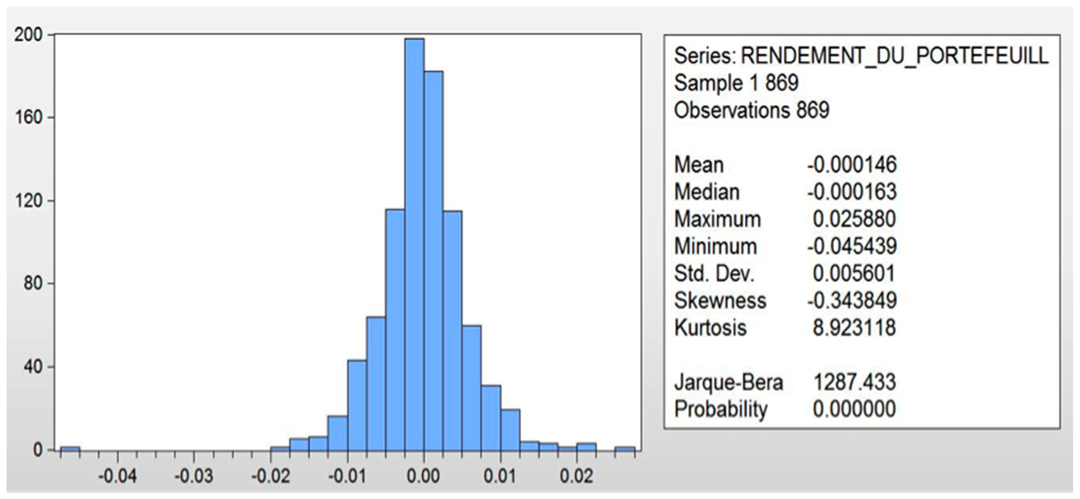
The test was carried out on Eviews with the following results.

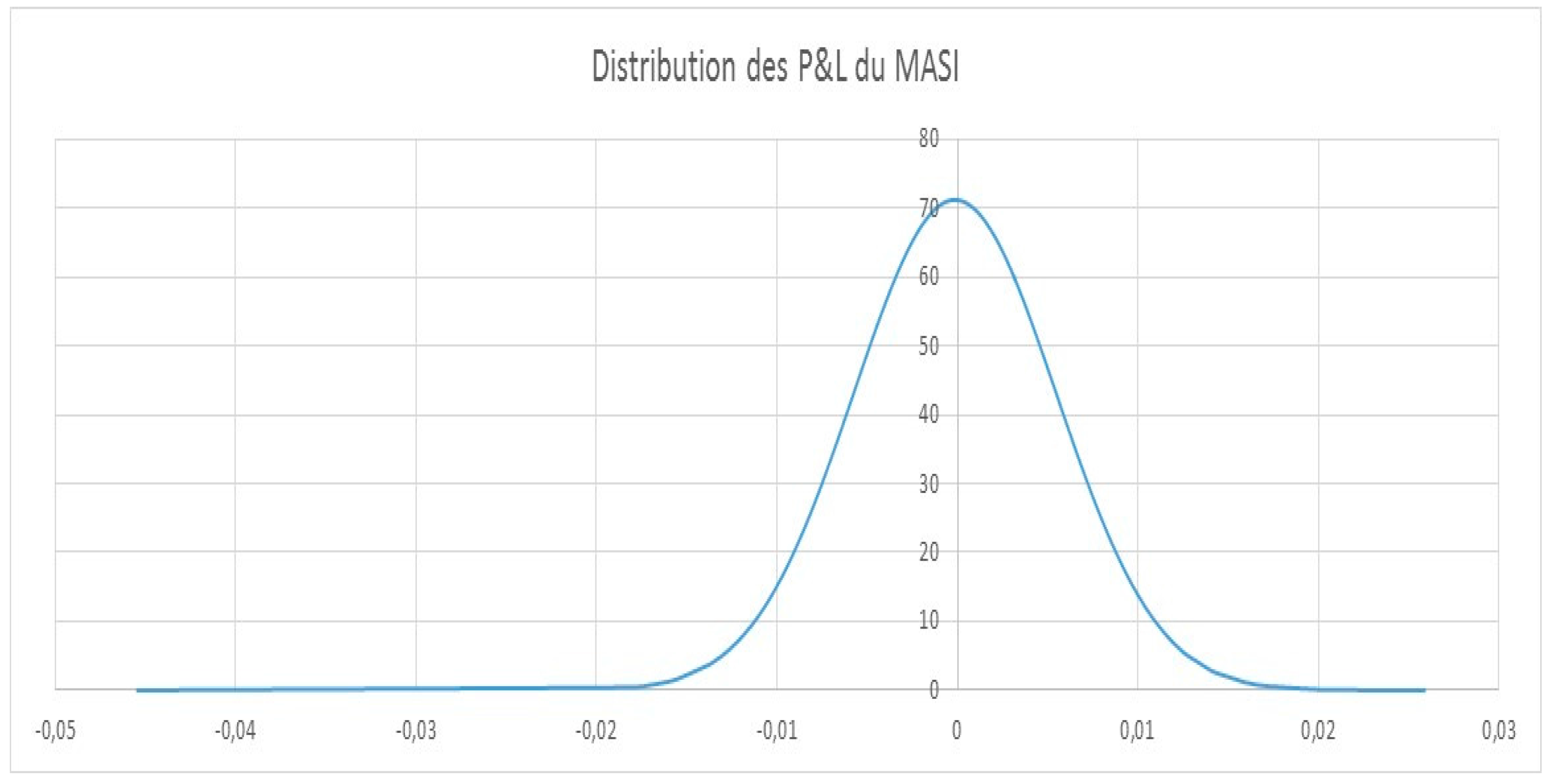
Referring to the Jarque–Bera statistics displayed in Figure 1, we can see that the p-value displayed is 0 < 0.05 where the confidence threshold is fixed. Thus, we reject the hypothesis $H_0$. Hence, the distribution is not normal (see in Figure 2).

Since the distribution is not normal, it would therefore be wrong to calculate the VaR based on this assumption because the amount that the VaR will display may be underestimated or overestimated depending on the characteristics of the distribution (Leptocurtic, platicurtic, etc.) [13]. However, in order to see the desired effect, it must be assumed that the distribution of risk factors in the portfolio follows a normal distribution pattern. We will calculate the VaR based on this hypothesis; then, we will propose an adjustment to extract the true quantile related to our distribution and recalculate the VaR.

Once these elements are available, and assuming a normal distribution, the parametric VaR is obtained from Equation (16).

The portfolio is made up of several assets; therefore,

$$\sigma \left(R\right)=\sqrt{{\omega }^t \Sigma \omega }$$

(57)

where

• $\Sigma :\mathrm{variance}–\mathrm{covariance}$ matrix;
• $\Omega :\mathrm{weight}\mathrm{vector}$;
• ${\omega }^t:\mathrm{the}\mathrm{transposition}\mathrm{of}\mathrm{the}\mathrm{weight}\mathrm{vector}$.

If we recall the distinction between absolute VaR and relative VaR, we obtain (see in

Table 3. Matrix Variance–Covariance of the securities making up the MASI portfolio.

Stocks	Afriquia GAZ	Afriqia Industrie	…	Alliance	Wafa Assur
Afriquia GAZ	0.0003123	0.0000004	…	0.0000110	0.0000153
Afriqia industrie	0.0000004	0.0002066	…	0.0000144	−0.0000151
…	…	…	…	…	…
Alliance	0.0000110	0.0000144	…	0.0002081	0.0000224
Wafa assur	0.0000153	−0.0000151	…	0.0000224	0.0004371

Table produced on Excel under VBA by the authors.

):

$$\mathrm{Absolute}\mathrm{VaR}=\mathrm{Relative}\mathrm{VaR}-\mathrm{Expected}\mathrm{average}\mathrm{portfolio}\mathrm{yield}.$$

The application of parametric VaR to the MASI portfolio gives the results shown in

Table 4. Parametric VaR calculation for 30 June 2017 (under assumption of normality).

VaR Parameters	Parametric Value at Risk
	Relative		Absolute
	%	MAD	%	MAD
VaR (95%,1-day)	−0.92%	−1,041,208,988.18 MAD	−0.91%	−1,024,691,792.13 MAD
VaR (99%,1-day)	−1.31%	−1,472,601,741.82 MAD	−1.29%	−1,456,084,545.77 MAD
VaR (95%,10-days)	−2.91%	−3,292,591,922.90 MAD	−2.87%	−3,240,359,962.80 MAD
VaR (99%,10-days)	−4.12%	−4,656,775,590.49 MAD	−4.07%	−4,604,543,630.40 MAD

Table produced on Excel under VBA by the authors.

.

Based on the assumption of normality, the VaR at the 95% threshold over 1 day displays ${\mathrm{VaR}}_{0.95;1}=1041.21\mathrm{MMAD}$. This means that we are 95% sure that the loss that our MASI portfolio will suffer will not exceed the amount the VaR will post on the next day—that is, 0.9213% of the total value of the portfolio, for a confidence level of 99%. The parametric VaR is 1472.60 MMAD.

As already noted in the calculation of the historical VaR, the change from a 1 day investment horizon to a 10 day investment horizon implies a clear increase in the amount to be lost on the MASI portfolio (3292.59 MMAD for 95% confidence and 4656.76 MMAD for a 99% confidence level).

3.1.3. Cornish–Fischer Expansion or Adjustment

Generally, to simplify calculations, the distribution of risk factors is assumed to be normal. However, this assumption is rarely actually verified; this can skew the estimation of the actual VaR value as mentioned above.

Indeed, there are adjustments that allow us to more closely approach the true value of VaR. Cornish–Fischer adjustment is the most common [14], and is an approximate relationship between the percentiles of a distribution and its moments (expectation, standard deviation, Skewness, and Kurtosis).

This approximation is based on the Taylor series and uses the moments of a distribution that deviates from normal to calculate its percentiles. The expansion of Cornish–Fisher is written as follows [14]:

$$W_{1-\alpha }= Z_{1-\alpha }-\left(\frac{1}{6}\right)\left(Z_{1-\alpha }^2-1\right)S+(\frac{1}{24})\left(Z_{1-\alpha }^3-3Z_{1-\alpha }\right)EKur-(\frac{1}{36})\left(2Z_{1-\alpha }^3-5Z_{1-\alpha }\right)S^2$$

(58)

where $Z_{1-\alpha }$ is the quantile of the normal law, $S$ is the asymmetry coefficient, and $\mathrm{EKUR}$ is the excess of kurtosis which is equal to the flattening coefficient −3.

Therefore, instead of relying on the quantile taken from the normal law, the latter will be replaced by the corrected quantile [15]. Equation (16) becomes

$$\mathrm{VaR}=W_{1-\alpha }\ast \sigma \left(R\right)-E\left(R\right).$$

(59)

Based on the distribution of returns of the MASI portfolio we found

• $S = -0.3438$ (asymmetry coefficient);
• $K = 8.92318$ (flattening coefficient).

The Cornish–Fisher fit shows that the quantile corrected to the 95% and 99% threshold, respectively, is equal to

$$W_{0.05}=- 1.6807{\mathrm{and}\mathrm{W}}_{0.01}=-3.22.$$

These adjustment results shown in

Table 5. Parametric VaR calculation for 30 June 2017.

VaR Parameters	Adjusted Parametric Value at Risk
	Relative		Absolute
	%	MAD	%	MAD
VaR (95%,1-day)	−0.94%	−1,063,909,251.02 MAD	−0.93%	−1,047,392,054.96 MAD
VaR (99%,1-day)	−1.81%	−2,043,346,992.54 MAD	−1.79%	−2,026,829,796.48 MAD
VaR (95%,10-days)	−2.98%	−3,364,376,456.94 MAD	−2.93%	−3,312,144,496.84 MAD
VaR (99%,10-days)	−5.72%	−6,461,630,546.48 MAD	−5.67%	−6,409,398,586.38 MAD

Table produced on Excel under VBA by the authors.

are clearly superior to the data from the normal law table ($Z_{0.05}=1.644$ and $Z_{0.01}= -2.33$).

According to the above calculations, the adjusted VaR is higher than that calculated based on the assumption of normality. Thus, in our case, the calculations have led to an underestimation of the amount of the potential loss under the assumption of normalcy.

3.1.4. Application of Monte Carlo VaR to the MASI Portfolio

The application of Monte Carlo VaR to the MASI portfolio gives the results shown in

Table 6. Monte Carlo VaR Calculation for 30 June 2017.

VaR Parameters	Monte Carlo Value at Risk
	%	MAD
VaR (95%,1-day)	−1.04%	1,178,476.625.61 MAD
VaR (99%,1-day)	−1.48%	1,669,542,616.39 MAD
VaR (95%,10-days)	−3.30%	3,726,670,306.19 MAD
VaR (99%,10-days)	−4.67%	5,279,557,318.51 MAD

Table produced on Excel under VBA by the authors.

.

Table 6 shows the maximum loss calculations that can be made if we keep our MASI portfolio unchanged. For a duration of 1 day, the maximum loss is 1602.58 MMAD with a probability of 95% (for the 99% confidence level, the maximum loss is 1987.81 MMAD).

On the other hand, for 10 days, there is only a 1% chance that our loss exceeds 6286.01 MMAD and only a 5% chance that the loss exceeds 5067.81 MMAD.

In conclusion, the VaR calculation reveals that it is of paramount importance in judging the levels of risk to be faced on the Casablanca financial market. However, this risk measure does not provide any information on the severity of the loss, nor does it provide information on the extent of extreme losses beyond the VaR.

It is also important to note that the amounts of losses estimated by the various VaR methods are still to be discussed according to the level of risk aversion and the quality of fund managers (speculator; long-term investor termites, capital risk; private individual), and again, according to the levels of returns to be obtained on the financial market [16].

3.1.5. Application of PVaR to the MASI Portfolio

A decomposition of VaR, showing the securities [17] that contribute most to the loss, is given in

Table 7. Lists of the 12 stocks contributing most significantly to the loss.

Stocks	PVaR Contribution
Attijariwafa bank	−0.271%
Itissalat al maghrib	−0.241%
Lafarge ciments	−0.180%
Cosumar	−0.130%
Holcim maroc	−0.070%
Bmce bank	−0.070%
BCP	−0.060%
Douja prom addoha	−0.050%
Ciments du maroc	−0.050%
Wafa assurance	−0.040%
CGI	−0.020%
Managem	−0.020%

Table produced on Excel under VBA by the authors.

.

The sum of the calculated PVaR gives

$${\displaystyle \sum }_{i=1}^{75}{\mathrm{PVaR}}_{95\%}=-1,040,010,819.04\mathrm{MAD},$$

and the calculated VaR gives

$${\mathrm{VaR}}_{0.95}=-1,024,691,792.18\mathrm{MAD}.$$

The difference in the sum of the PVaR and the calculated VaR gives the following result:

$$\mathrm{Ecart}\left({\mathrm{VaR}}_{0.95},{\displaystyle \sum }_{i=1}^{74}{\mathrm{PVaR}}_{95\%}\right)=-2,064,702,611.16\mathrm{MAD}.$$

However, the ratio between the sum of the PVaR and the VaR gives

$$\frac{{\mathrm{VaR}}_{0.95}}{{\sum }_{i=1}^{74}{\mathrm{PVaR}}_{95\%}}=99\%.$$

The objective of the PVaR calculation is to check whether the sum of the VaR of each security in the portfolio—taken independently—is greater than the overall VaR of the portfolio (diversification principle) [18]. That is a difference of 119,817 MMAD for our case study. The explanation for this difference is due to the reduction in the loss due to the intra-portfolio correlation (clearing) effect.

The VaR assessment of the loss based on the contributions of each value in the MASI portfolio is mainly due to two factors.

The weighting element in capitalization is dominated by the telecom sector (IAM), banks (AATTIJARI, BCP), and the cement industry (LAFARGE, CIMENT of Morocco, and HOLCIM). These securities make up the bulk of the MASI portfolio; hence, any bearish movement in these securities will contribute to VaR loss.

The volatility element concerns mainly ADDOHA, CGI, and MANAGEM stocks, which are the most volatile stocks on the market. The two real estate sector values (ADDOHA and CGI) stem essentially from a market effect underpinned by an abundance of economic information, and very volatile demand. This results in probabilities of losses and gains exceeding the loss recorded by VaR calculations. In the case of MANAGEM, this is a highly volatile value due to its sector of activity, which is based on mining operations.

3.2. Modelling by ETL

3.2.1. Application of Historical ETL to the MASI Portfolio

Along with VaR, the historical ETL method is the easiest to use, since it is based on the assumption that the various risk factors are stationary.

The ETL threshold $\alpha$ is defined as a measure of the mean of the most important losses from those given by $\mathrm{VaR}\left(\alpha \right).$ Thus, the direct methodology of the historical ETL calculation with an $a=\alpha \%$ confidence level assumes that we have a sample of profits/losses $X_1\dots X_n$, which is sorted in ascending order $X_{\left[1\right]}<X_{\left[2\right]}<\dots <X_{\left[N\right]}$. The mathematical formulation of the historical ETL is denoted as follows:

$$ET{L}_{\alpha }\left(X\right)=\frac{1}{\left[N.\alpha \right]}{\displaystyle \sum }_{i=1}^{\left[N.\alpha \right]}{X}_{\left[i\right]}.$$

(60)

The results of the application of historical ETL to the MASI portfolio are shown in

Table 8. Calculation of the historical Expected Tail Loss (ETL) for 30 June 2017.

VaR Parameters	Monte Carlo Value at Risk
	%	MAD
VaR (95%,1-day)	−1.2282%	−1,388,012,915.66 MAD
VaR (99%,1-day)	−1.9215%	−2,171,479,166.29 MAD
VaR (95%,10-days)	−3.8840%	−4,389,282,235.23 MAD
VaR (99%,10-days)	−6.0763%	−6,866,820,057.09 MAD

Table produced on Excel under VBA by the authors.

.

Compared with the results given by the historical VaR, the historical ETL shows us a quantification of the amounts to be lost that are more important, which explains why the expected loss provided is higher than that given by the VaR. This increase in losses is caused by the occurrence of extreme events. In the case of our MASI portfolio, the above results show a portfolio value depreciation of more than 1.23% at the 95% threshold over a 1 day horizon and 1.92% for a 99% confidence level. However, for an investment horizon of 10 days, the amounts to be lost are more colossal, given as a percentage of the depreciations: 3.88% for a confidence level of 95%, and 6.08% for 99% of confidence.

3.2.2. Application of Parametric ETL to the MASI Portfolio

The parametric ETL method is based on the assumption that the distribution of underlying market factors is normal. However, although this hypothesis has the advantage of considerably simplifying the ETL estimate, it nevertheless has the disadvantage of not being very empirically realistic.

Thus, it is possible to obtain the parametric ETL by the following formula:

$$ETL\left(X,\alpha \right)=E\left[-X|-X\ge VAR\left(X,\alpha \right)\right],$$

(61)

$$ETL\left(X,\alpha \right)=\frac{{\sigma }_x}{\alpha \sqrt{2\pi }}e\frac{-q_{\alpha }^2}{2}.$$

(62)

The results of the application of this method to the MASI portfolio are shown in

Table 9. Calculation of the parametric ETL for 28 June 2017.

VaR Parameters	Monte Carlo Value at Risk
	%	MAD
VaR (95%,1-day)	−1.16%	−1,305,718,077.30 MAD
VaR (99%,1-day)	−1.49%	−1,687,107,567.62 MAD
VaR (95%,10-days)	−3.65%	−4,129,043,106.32 MAD
VaR (99%,10-days)	−4.72%	−5,335,102,571.39 MAD

Table produced on Excel under VBA by the authors.

.

In the same configuration of calculations and results obtained for the historical ETL, the losses to be faced in our MASI portfolio are consistent with the principle that the ETL is superior to VaR. Thus, the devaluation of the MASI portfolio is further driven by extreme events with a 99% confidence level and a 1 day investment horizon that clearly depreciates by 1.49% of the total value of the portfolio.

3.2.3. Application of Monte Carlo ETL to the MASI Portfolio

As far as the Monte Carlo method is concerned, the principle remains the same as the historical ETL. However, the Monte Carlo method is based on upstream-generated simulations to calculate the Monte Carlo VaR. The ETL corresponding to a chosen probability level must then be extracted. This is done, in fact, by the same formula as for the historical ETL, i.e., by calculating the average of the estimated losses knowing that these losses exceed the maximum loss, which is the VaR.

$$ET{L}_{\alpha }\left(X\right)=\frac{1}{\left[N.\alpha \right]}{\displaystyle \sum }_{i=1}^{\left[N.\alpha \right]}{X}_{\left[i\right]}$$

(63)

Applying this method (ETL Monte Carlo) to the MASI portfolio gives us the results shown in

Table 10. Calculation of the Monte Carlo ETL for 30 June 2017.

VaR Parameters	Monte Carlo Value at Risk
	%	MAD
VaR (95%,1-day)	−1.23277%	1,393,158,385.82 MAD
VaR (99%,1-day)	−1.47733%	1,669,542,616.39 MAD
VaR (95%,10-days)	−3.89835%	4,405,553,640.55 MAD
VaR (99%,10-days)	−4.67170%	5,279,557,318.51 MAD

Table produced on Excel under VBA by the authors.

.

According to the Monte Carlo ETL calculation method for a 1 day investment horizon and a ceiling threshold of 5%, the extreme parts of the distribution of risk factors show a maximum loss of 1393.159 MMAD, i.e., a devaluation of 1.233% of our MASI portfolio. This maximum loss is revised upwards (in absolute terms) for a narrower confidence level (1669.543 MMAD loss for 1% default).

4. Discussion

We have analyzed and tested the ETL approach for the VaR in the Moroccan stock market portfolio. We have compared the results with the general approaches to the general VaR, which has been the most suitable method for Moroccan stock investors up to now. In the same order of analysis as the previous methods, generally, the investment horizon remains in positive correlation with the probable loss incurred for any investment in the MASI portfolio. This is explained by the accumulation of daily loss probabilities.

Besides the fact that these methods present an easy and fast implementation, it is important to note the large amount of data required to undertake the calculation of VaR, the expected returns and variances of each asset, as well as the covariances between assets. Normally, a risk manager will have access to historical performance data for each asset, so that only a few lines of code are needed to calculate expected returns, spreads, and covariances.

It is also important to note that the VaR is a very versatile model. Although a normal distribution is used in our study, practically any distribution can be implemented. This gives the risk manager the opportunity to adapt a VaR model for the specific characteristics of the implemented portfolio.

Finally, an interesting trend in risk management has been the movement towards probability distributions that have “thicker tails”. A major achievement of the recent financial crisis has been that the financial impact is not always modeled by a normal or other benign distribution. Extreme events, often called “black swans”, tend to occur more frequently than these distributions would expect.

As an acknowledgement of the application of the ETL to measure and quantify loss in the Moroccan financial market, it is noted that this market is no longer immune to an above-average volatility. This will increase the likelihood of extreme parties and automatically lead to colossal losses for investors. This brings us back to the risk aversion of the various investors and also to the adequacy of the relationship between the risks of loss on the Moroccan stock market, which is constantly increasing, and the levels of returns expected on this stock market, which remain well below investors’ expectations.

5. Conclusions

VaR is an essential indicator in risk management today. It was, in fact, highly popularized in the 1990s and subsequently became inevitable in usage, since VaR appears in the Basel II agreements as the preferred method of risk measurement. Despite this ease of understanding and the major advantages it possesses, VaR has some disadvantages, namely its inconsistency and the fact that it does not take into account rare (extreme) phenomena. However, to remedy these limitations, the mathematical and financial development of VaR has given rise to an alternative measure, known as the ETL. ETL is a measure similar to VaR in terms of modeling but is more precise in terms of calculation since it incorporates the extreme values that have become a decisive issue for fund managers in the current financial market context [19].

In addition, by focusing our interest on the MASI, the market portfolio, because of its broad representation in Casablanca and its ability to integrate all securities listed on the Moroccan stock exchange, the aim was to quantify the amounts to be lost in the financial market using two approaches—the VaR and the ETL. The quantification of the amounts to be lost makes it possible to judge the volatility of the market and, consequently, to offer investors the opportunity to choose to invest in the MASI portfolio, if not deciding to seek investment elsewhere.

Thus, at the end of our research on Casablanca’s quotation space, we came to the following conclusions:

(i)

The loss to be faced depends on the narrowness of the Moroccan stock market (a small number of sectors and quoted securities). In other words, few stocks create intense volatility across the entire portfolio. Indeed, the first five values in terms of weight alone account for more than 80% of the total loss calculated on the basis of the two approaches (VaR and ETL).

(ii)

The downward trend in the stock market from 2009 to June 2016 sets out the risk to be undertaken in any investment in the MASI portfolio. This is consolidated by our VaR and ETL calculations, which show significant levels of losses compared with the mixed returns on the various subfunds of the Moroccan financial market.

The results of this research are confirmed by the reports of the Casablanca Stock Exchange on the volumes traded between investors and the level of liquidity. Indeed, the Moroccan stock market is characterized by a possible absence of investment opportunities and a plausible disinterest of investors in relation to investments on the Casablanca Stock Exchange.

References

- Markowitz, H. Portfolio Selection: Efficient Diversification of Investments; John Wiley & Pte. Ltd.: Hoboken, NJ, USA, 1959. [Google Scholar]
- Bodson, L.; Grandin, P.; Hübner, G.; Lambe, M. Performance de Portefeuille, 2nd ed.; Pearson Education: Paris, France, 2010. [Google Scholar]
- Linsmeier, T.J.; Pearson, N.D. Value at Risk. Financ. Anal. 2000, 56, 47–67. [Google Scholar] [CrossRef]
- Esch, K. Value at Risk: Vers un Risk Management Moderne; De Boeck: Paris, France, 1997. [Google Scholar]
- Artzner, D.; Eber, H. Coherent measures of risk. Math. Financ. 1999, 9, 203–228. [Google Scholar] [CrossRef]
- Wijst, N.V. Finance: A Quantitative Introduction; Cambridge University Press: Cambridge, MA, USA, 2013. [Google Scholar]
- Béchu, T. Économie et Marchés Financiers: Perspectives 2010–2020; Eyrolles: Paris, France, 2010. [Google Scholar]
- Hallerbach, W.G. Decomposing Portfolio Value-at-Risk: A General Analysis. J. Risk 2003, 5, 13–43. [Google Scholar] [CrossRef]
- Markowitz, H. Portfolio Selection. Finance 1952, 7, 77–91. [Google Scholar]
- Carole, A. Market Risk Analysis: Value-At-Risk Models; John Wiley & Sons Ltd.: Hoboken, NJ, USA, 2008. [Google Scholar]
- Hull, J. Gestion des Risques et Institutions Financière, 2nd ed.; Pearson Education: Paris, France, 2010. [Google Scholar]
- Sirr, G.; Garvey, J.; Gallagher, L. Emerging markets and portfolio foreign exchange risk: An empirical investigation using a value-at-risk decomposition technique. Int. Money Financ. 2011, 30, 1749–1772. [Google Scholar] [CrossRef]
- David, X. Value at Risk Based on the Volatility Skewness and Kurtosis; Riskmetrics Group: New York, NY, USA, 1999. [Google Scholar]
- Charles, O.; Manesme, A.; Barthélémy, F. Expansion fir Real Estate Value at Risk. In Proceedings of the European Real Estate Society Annual Conference, Edinburgh, Scotland, 13–16 June 2012. [Google Scholar]
- Fama, E.; Macbeth, J. Risk, return and equilibrium: Empirical tests. Political Econ. 1973, 81, 607–636. [Google Scholar] [CrossRef]
- Pearson, N.D. Risk Budgeting: Portofolio Problem Solving with Value-at-Risk; John Wiley & Pte. Ltd.: Hoboken, NJ, USA, 2002. [Google Scholar]
- Casablanca Stock Exchange. Available online: http://www.casablanca-bourse.com/bourseweb/en/index.aspx (accessed on 15 July 2017).
- Assaf, A. Value-at-Risk Analysis in the MENA Equity Markets: Fat Tails and Conditional Asymmetries in Return Distributions. Multinatl. Financ. Manag. 2015, 29, 30–45. [Google Scholar] [CrossRef]
- Moraux, F. How valuable is your VaR? Large sample confidence intervals for normal VaR. Risk Manag. Financ. Inst. 2011, 4, 189–200. [Google Scholar]
Figure 1.
Jarque–Bera test statistics.
Figure 2.
Moroccan All Shares Index (MASI) profits and losses (P&L) distribution.