Data Driven Economic Model Predictive Control


Department of Chemical Engineering, McMaster University, Hamilton, ON L8S 4L7, Canada
*
Author to whom correspondence should be addressed.
Mathematics 2018, 6(4), 51; https://doi.org/10.3390/math6040051
Submission received: 7 March 2018
/
Revised: 21 March 2018
/
Accepted: 22 March 2018
/
Published: 2 April 2018
(This article belongs to the Special Issue New Directions on Model Predictive Control)
Abstract
:This manuscript addresses the problem of data driven model based economic model predictive control (MPC) design. To this end, first, a data-driven Lyapunov-based MPC is designed, and shown to be capable of stabilizing a system at an unstable equilibrium point. The data driven Lyapunov-based MPC utilizes a linear time invariant (LTI) model cognizant of the fact that the training data, owing to the unstable nature of the equilibrium point, has to be obtained from closed-loop operation or experiments. Simulation results are first presented demonstrating closed-loop stability under the proposed data-driven Lyapunov-based MPC. The underlying data-driven model is then utilized as the basis to design an economic MPC. The economic improvements yielded by the proposed method are illustrated through simulations on a nonlinear chemical process system example.
1. Introduction
Control systems designed to manage chemical process operations often face numerous challenges such as inherent nonlinearity, process constraints and uncertainty. Model predictive control (MPC) is a well-established control method that can handle these challenges. In MPC, the control action is computed by solving an open-loop optimal control problem at each sampling instance over a time horizon, subject to the model that captures the dynamic response of the plant, and constraints [1]. In early MPC designs, the objective function was often utilized as a parameter to ensure closed-loop stability. In subsequent contributions, Lyapunov-based MPC was proposed where feasibility and stability from a well characterized region was built into the MPC [2,3].
With increasing recognition (and ability) of MPC designs to focus on economic objectives, the notion of Economic MPC (EMPC) was developed for linear and nonlinear systems [4,5,6], and several important issues (such as input rate-of-change constraint and uncertainty) addressed. The key idea with the EMPC designs is the fact that the controller is directly given the economic objective to work with, and the controller internally determines the process operation (including, if needed, a set point) [7].
Most of the existing MPC formulations, economic or otherwise, have been illustrated using first principles models. With growing availability of data, there exists the possibility of enhancing MPC implementation for situations where a first principles model may not be available, and simple ‘step-test’, transfer-function based model identification approaches may not suffice. One of the widely utilized approaches in the general direction of model identification are latent variable methods, where the correlation between subsequent measurements is used to model and predict the process evolution [8,9]. In one direction, Dynamic Mode Decomposition with control (DMDc) has been utilized to extract low-order models from high-dimensional, complex systems [10,11]. In another direction, subspace-based system identification methods have been adapted for the purpose of model identification, where state-space model from measured data are identified using projection methods [12,13,14]. To handle the resultant plant model mismatch with data-driven model based approaches, monitoring of the model validity becomes especially important.
One approach to monitor the process is to focus on control performance [15], where the control performance is monitored and compared against a benchmark control design. To focus more explicitly on the model behavior, in a recent result [16], an adaptive data-driven MPC was proposed to evaluate model prediction performance and trigger model identification in case of poor model prediction. In another direction, an EMPC using empirical model was proposed [17]. The approach relies on a linearization approach, resulting in closed-loop stability guarantees for regions where the plant-model mismatch is sufficiently small, and illustrate results on stabilization around nominally stable equilibrium points. In summary, data driven MPC or EMPC approaches, which utilize appropriate modeling techniques to identify data from closed-loop tests to handle operation around nominally unstable equilibrium points, remain to be addressed.
Motivated by the above considerations, in this work, we address the problem of data driven model based predictive control at an unstable equilibrium point. In order to identify a model around an unstable equilibrium point, the system is perturbed under closed-loop operation. Having identified a model, a Lyapunov-based MPC is designed to achieve local and practical stability. The Lyapunov-based design is then used as the basis for a data driven Lyapunov-based EMPC design to achieve economical goals while ensuring boundedness. The rest of the manuscript is organized as follows: first, the general mathematical description for the systems considered in this work and a representative formulation for Lyapunov-based model predictive control are presented. Then, the proposed approach for closed-loop model identification is explained. Subsequently, a Lyapunov-based MPC is designed and illustrated through a simulation example. Finally, an economic MPC is designed to consider economical objectives. The efficacy of the proposed method is illustrated through implementation on a nonlinear continuous stirred-tank reactor (CSTR) with input rate of change constraints. Finally, concluding remarks are presented.
2. Preliminaries
This section presents a brief description of the general class of processes that are considered in this manuscript, followed by closed-loop subspace identification and Lyapunov based MPC formulation.
2.1. System Description
We consider a multi-input multi-output (MIMO) controllable systems where denotes the vector of constrained manipulated variables, taking values in a nonempty convex subset , where , and denote the lower and upper bounds of the input variables, and denotes the vector of measured output variables. In keeping with the discrete implementation of MPC, u is piecewise constant and defined over an arbitrary sampling instance k as:
where is the sampling time and and denote state and output at the kth sample time. The central problem that the present manuscript addresses is that of designing a data driven modeling and control design for economic MPC.
2.2. System Identification
In this section, a brief review of a conventional subspace-based state space system identification methods is presented [16,18,19]. These methods are used to identify the system matrices for a discrete-time linear time invariant (LTI) system of the following form:
where and denote the vectors of state variables and measured outputs, and and are zero mean, white vectors of process noise and measurement noise with the following covariance matrices:
where , and are covariance matrices, and is the Kronecker delta function. The subspace-based system identification techniques utilize Hankel matrices constructed by stacking the output measurements and manipulated variables as follows:
where i is a user-specified parameter that limits the maximum order of the system (n), and, j is determined by the number of sample times of data. By using Equation (4), the past and future Hankel matrices for input and output are defined:
Similar block-Hankel matrices are made for process and measurement noises and are defined in the similar way. The state sequences are defined as follows:
Furthermore, these matrices are used in the algorithm:
By recursive substitution into the state space model equations Equations (1) and (2), it is straightforward to show:
where:
Equation (9) can be rewritten in the following form to have the input and output data at the left hand side of the equation [20]:
In open loop identification methods, in the next step, by orthogonal projecting of Equation (15) onto :
Note that, the last two terms in RHS of Equation (15) are eliminated since the noise terms are independent, or othogonal to the future inputs. Equation (16) indicates that:
Therefore, and can be calculated using Equation (17) by decomposition methods. These can in turn be utilized to determine the system matrices (some of these details are deferred to Section 3.1). For further discussion on system matrix extraction, the readers are referred to references [18,19].
2.3. Lyapunov-Based MPC
The Lyapunov-based MPC (LMPC) for linear system has the following form:
where , , and denote predicted state and output, output set-point and calculated manipulated input variables j time steps ahead computed at time step k, and is the current estimation of state, and is a user defined parameter. The operator denotes the weighted Euclidean norm defined for an arbitrary vector x and weighting matrix W as . Furthermore, and denote the positive definite and positive semi-definite weighting matrices for penalizing deviations in the output predictions and for the rate of change of the manipulated inputs, respectively. Moreover, and denote the prediction and control horizons, respectively, and the input rate of change, given by , takes values in a nonempty convex subset , where . Note finally that, while the system dynamics are described in continuous time, the objective function and constraints are defined in discrete time to be consistent with the discrete implementation of the control action.
Equations (23) and (24) are representatives of Lyapunov-based stability constraint [21,22], where is a suitable control Lyapunov function, and are user-specified parameters. In the presented formulation, enables practical stabilization to account for the discrete nature of the control implementation.
Remark 1.
Existing Lyapunov-based MPC approaches exploit the fact that the feasibility (and stability) region can be pre-determined. The feasibility region, among other things, depends on the choice of the parameter α, the requested decay factor in the value of the Lyapunov function at each time step. If (reasonably) good first principles models are available, then these features of the MPC formulation provide excellent confidence over the operating region under closed-loop. In contrast, in the presence of significant plant-model mismatch (as is possibly the case with data driven models), the imposition of such decay constraints could result in unnecessary infeasibility issues. In designing the LMPC formulation with a data driven model, this possible lack of feasibility must be accounted for (as is done in Section 3.2).
3. Integrating Lyapunov-Based MPC with Data Driven Models
In this section, we first utilize an identification approach necessary to identify good models for operation around an unstable equilibrium point. The data driven Lyapunov-based MPC design is presented next.
3.1. Closed-Loop Model Identification
Note that, when interested in identifying the system around an unstable equilibrium point, open-loop data would not suffice. To begin with, nominal open-loop operation around an unstable equilibrium point is not possible. If the nominal operation is under closed-loop, but the loop is opened to perform step tests, the system would move to the stable equilibrium point corresponding to the new input value, thereby not providing dynamic information around the desired operating point. The training data, therefore, has to be obtained using closed-loop step tests, and an appropriate closed-loop model identification method employed. Such a method is described next.
In employing closed-loop data, note that the assumption of future inputs being independent of future disturbances no longer holds, and, if not recognized, can cause biased results in system identification [18]. In order to handle this issue, the closed-loop identification approach in the projection utilizes a different variable instead of . The new instrument variable, which satisfies the independence requirement, is used to project both sides of Equation (15) and the result is used to determine LTI model matrices. For further details, refer to [16,18,23].
By projecting Equation (15) onto we get:
Since the future process and measurement noises are independent of the past input/output and future setpoint in Equation (25), the noise terms cancel, resulting in:
By multiplying Equation (26) by the extended orthogonal observability , the state term is eliminated:
Therefore, the column space of is orthogonal to the row space of . By performing singular value decomposition (SVD) of :
where contains dominant singular values of and, theoretically, it has the order [18,23].
Therefore, the order of the system can be determined by the number of the dominant singular values of the [20]. The orthogonal column space of is , where is any constant nonsingular matrix and is typically chosen as an identity matrix [18,23]. One approach to determine the LTI model is as follows [18]:
From Equation (29), and can be estimated:
which results in (using MATLAB (2017a, MathWorks, Natick, MA, USA) matrix index notation):
The past state sequence can be calculated as follows:
The future state sequence can be calculated by changing data Hankel matrices as follows [18]:
where is obtained by eliminating the last rows of , and is obtained by eliminating the last rows and the last columns of . Then, the model matrices can be estimated using least squares:
Note that the difference between the proposed method in [18] and described method is that, in order to ensure that the observer is stable (eigenvalues of are inside unit circle), instead of innovation form of LTI model, Equations (1) and (2) are used [16] to derive extended state space equations. The system matrices can be calculated as follows:
With the proposed approach, process and measurement noise Hankel matrices can be calculated as the residual of the least square solution of Equation (39):
Then, the covariances of plant noises can be estimated as follows:
Model identification using closed-loop data has a positive impact on the predictive capability of the model (see the simulation section for a comparison with a model identified using open-loop data).
3.2. Control Design and Implementation
Having identified an LTI model for the system (with its associated states), the MPC implementation first requires a determination of the state estimates. To this end, an appropriate state estimator needs to be utilized. In the present manuscript, a Luenberger observer is utilized for the purpose of illustration. Thus, at the time of control implementation, state estimates are generated as follows:
where L is the observer gain and is computed using pole placement method, and is the vector of measured variables (in deviation form, from the set point).
In order to stabilize the system at an unstable equilibrium point, a Lyapunov-based MPC is designed. The control calculation is achieved using a two-tier approach (to decouple the problem of stability enforcement and objective function tuning). The first layer calculates the minimum value of Lyapunov function that can be reached subject to the constraints. This tier is formulated as follows:
where , are predicted state and output and is the candidate input computed in the first tier. is underlying state setpoint (in deviation form from the nominal equilibrium point), which here is the desired unstable equilibrium point (and therefore zero in terms of deviation variables). For setpoint tracking, this value can be calculated using the target calculation method; readers are referred to [24] for further details.
Note that the first tier has a prediction horizon of 1 because the objective is to only compute the immediate control action that would minimize the value of the Lyapunov function at the next time step. V is chosen as a quadratic Lyapunov function with the following form:
where P is a positive definite matrix computed by solving the Riccati equation with the LTI model matrices as follows:
where and are positive definite matrices. Then, in the second tier, this minimum value is used as a constraint (upper bound for Lyapunov function value at the next time step). The second tier is formulated as follows:
where is the prediction horizon and denotes the control action computed by the second tier. In essence, in the second tier, the controller calculates a control action sequence that can take the process to the setpoint in an optimal fashion optimally while ensuring that the system reaches the minimum achievable Lyapunov function value at the next time step. Note that, in both of the tiers, the input sequence is a decision variable in the optimization problem, but only the first value of the input sequence of the second tier is implemented on the process. The solution of the first tier, however, is used to ensure and generate a feasible initial guess for the second tier. The two-tiered control structure is schematically presented in Figure 1.
Remark 2.
Note that Tiers 1 and 2 are executed in series and at the same time, and the implementation does not require a time scale separation. The overall optimization is split into two tiers to guarantee feasibility of the optimization problem. In particular, the first tier computes an input move with the objective function only focusing on minimizing the Lyapunov function value at the next time step. Notice that the constraints in the first tier are such that the optimization problem is guaranteed to be feasible. With this feasible solution, the second tier is used to determine the input trajectory that achieves the best performance, while requiring the Lyapunov function to decay. Again, since the second tier optimization problem uses the solution from Tier 1 to impose the stability constraint, feasibility of the second tier optimization problem, and, hence, of the MPC optimization problem, is guaranteed. In contrast, if one were to require the Lyapunov function to decay by an arbitrary chosen factor, determination of that factor in a way that guarantees feasibility of the optimization problem would be a non-trivial task.
Remark 3.
It is important to recognize that, in the present formulation, feasibility of the optimization problem does not guarantee closed-loop stability. A superfluous (and incorrect) reason is as follows: the first tier computes the control action that minimizes the value of the Lyapunov function at the next step, but does not require that it be smaller than the previous time step, leading to potential destabilizing control action. The key point to realize here, however, is that if such a control action were to exist (that would lower the value of the Lyapunov function at the next time step), the optimization problem would determine that value by virtue of the Lyapunov function being the objective function, and lead to closed-loop stability. The reasons closed-loop stability may not be achieved are two: (1) the current state might be such that closed-loop stability is not achievable for the system dynamics and constraints; and (2) due to plant model mismatch, where the control action that causes the Lyapunov function to decay for the identified model does not do so for the system in question. The first reason points to a fundamental limitation due to the presence of input constraints, while the second is due to the lack of availability of the ‘correct’ system dynamics, and as such will be true in general for data driven MPC formulations. Note that inclusion of a noise/plant model mismatch term in the model may help with the predictive capability of the model, however, unless a bound on the uncertainty can be assumed, closed-loop stability can not be guaranteed.
Remark 4.
Along similar lines, consider the scenario where, based on the model, and constraints, an input value exists for which is achievable. It can be readily shown that any solution computed by the first tier of the optimization problem would also result in by virtue of the objective function being the Lyapunov function at the next time step. Thus, in such a case, the explicit incorporation of the constraint (as is traditionally done in Lyapunov based MPC) does not help, and is not required. On the other hand, for the scenario where such an input does not exist, the inclusion of the constraint will cause the optimization problem to be infeasible. In contrast, in the proposed formulation, the MPC will compute a control action where the value of the Lyapunov function might be greater than the previous value, but greater by the smallest margin possible. The real impact of this phenomenon is in making the MPC formulation more pliable, especially when dealing with plant-model mismatch. In such scenarios, the proposed MPC continues to compute feasible (best possible, in terms of stabilizing behavior) solutions, and, should the process move into a region from where stabilization is possible, smoothly transits to computing stabilizing control action.
Remark 5.
In the current manuscript, we focus on the cases where a first principal model is not available. If a good first principles model was available, it could be utilized directly in a nonlinear MPC design, or linearized if one were to implement a linear MPC. In the case of linearization, the applicability would be limited by the region over which the linearization holds. In contrast, note that the model utilized in the present manuscript does not result from a linearization of a nonlinear model. Instead, it is a linear model, possibly with a higher number of states than the original nonlinear model, albeit identified, and applicable, over a ‘larger’ region of operation, compared to a linearized model.
Remark 6.
To account for possible plant-model mismatch, model validity can be monitored with model monitoring methods [16], resulting in appropriately triggering re-identification in case of poor model prediction. In another direction, in line with control performance monitoring approaches, the Lyapunov function value could be utilized. Thus, unacceptable increases in Lyapunov function value could be utilized as a means of triggering re-identification.
Remark 7.
As mentioned previously, in order to create rich training data around unstable operating points, closed-loop data must be generated. In turn, since open-loop methods result in biased estimation [25,26] in model identification, a suitable closed-loop identification method is utilized, and adapted to ensure that the model accurately captures the key dynamics.
4. Simulation Results
We next illustrate the proposed approach using a nonlinear CSTR example [27]. To this end, consider a CSTR where a first-order, exothermic and irreversible reaction of the form takes place. The mass and energy conservation laws results in the following mathematical model:
The description of the process variables and the values of the system parameters are presented in Table 1. The control objective is to stabilize the system at an unstable equilibrium point using inlet concentration, , and the rate of heat input, Q, while the manipulated inputs are constrained to be within the limits kmol/m3 and KJ/min, and the input rate is constrained as Kmol/m3 and KJ/min. We assume that both of the states are measured. The system has an unstable equilibrium point at Kmol/m3 and K. The goal is to stabilize the system at this equilibrium point. To this end, first an LTI model is identified using closed-loop data; then, an MPC is designed to stabilize the system at the unstable equilibrium point.
For system identification of the CSTR model, proportional–integral (PI) controllers (pairing with and T with Q) are implemented in the process. In particular, pseudo-random binary signals are used as set-points for PI controllers. The identified LTI model order is selected as and , in order to achieve the best fit in model prediction (using cross-validation). Note that these four states are the states of the identified LTI model. When dealing with setpoint tracking, these states can be augmented with additional states and utilized as part of an offset-free MPC design. Model validation results under a different set of set-point changes from training data are presented in Figure 2 and Figure 3. The identified system is unstable with absolute eigenvalues which has an eigenvalue outside unit circle. The unstable nature of the identified model is consistent with the operation of the system around the unstable equilibrium point.
For the model validation, initially, a steady state Kalman filter (gain calculated by the identification method) is utilized to update state estimate until min and after convergence of the states (gaged via convergence of the outputs), the model and the input trajectory (without the state estimator) are used to predict the future output. Figure 2 illustrates the results of the model validation, and compares against a model obtained from open-loop step pseudo-random binary sequence (PRBS) on the input. As expected, the model identified using closed-loop data predicts better.
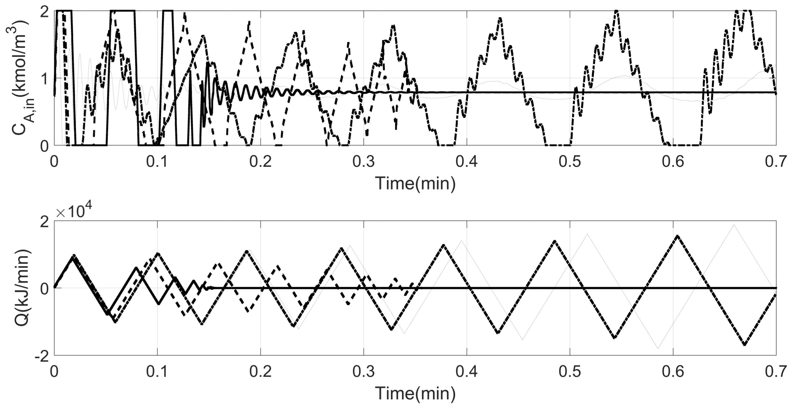
Next, closed-loop simulation results for proposed controller and conventional MPC (i.e., MPC without Lyapunov constraint) with horizons 1 and 10 are presented in Figure 4, Figure 5, Figure 6 and Figure 7. The controllers parameters are presented in Table 2. As can be seen, the LMPC has the best performance in stabilizing the system at the unstable equilibrium point. The MPC with a horizon of 1 is not capable of stabilizing the system, and the controller with a horizon of 10 reaches the set-point later compared to the LMPC. In addition, the evolution of the subspace states indicates better performance under the proposed LMPC.
5. Data-Driven EMPC Design and Illustration
Having illustrated the ability of the LMPC to achieve stabilization, it is next utilized to achieve economical objectives while ensuring stability. The Lyapunov based EMPC formulation is as follows:
where the value of dictates the neighborhood that the process states are allowed to evolve within. and indicate output and input cost vectors. Other variables have the same definition as Equation (47).
Remark 8.
In recent contributions [17,28], a Lyapunov-Based EMPC is proposed that utilizes data-driven methods to identify an empirical model for the system where the number of empirical model states is equal to the order of the plant model. In contrast, in the present work, the order of the model is selected based on the ability of the model to fit and predict dynamic behavior over a suitable range of operation, in turn allowing for an EMPC design that can reliably operate over a larger region.
Remark 9.
The EMPC formulation in the present manuscript utilizes a linear form of the cost function for the purpose of illustration. The proposed approach is not limited by this particular choice. Any other form of the cost function, including those where the costs could be time dependent, could be readily utilized within the proposed formulation. In such scenarios, the presence of the stability constraints provide the safeguards that allow the EMPC to move the process as needed to achieve economical goals.
Remark 10.
The use of linear models in the control design opens up the possibility of utilizing MPC formulations [3,29] that enable stabilization from the entire null controllable region (the region from which stabilization is achievable subject to input constraints). The use of the NCR can, in turn, be utilized to maximize the region over which the EMPC can be implemented, thereby maximizing the potential economic benefit. Such an implementation, however, needs to account for potential plant model mismatch owing to the use of the linear model, and remains the subject of future work.
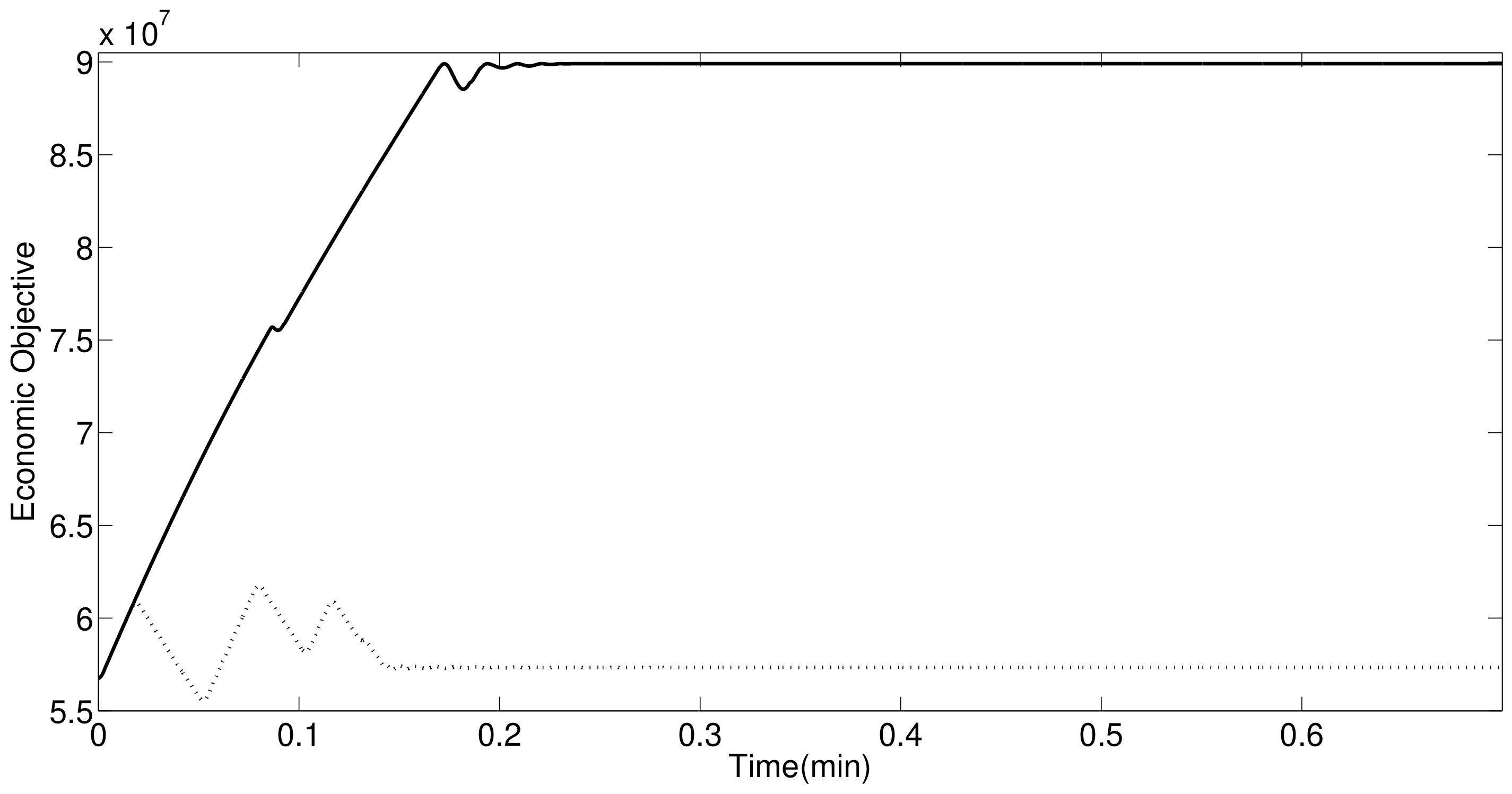
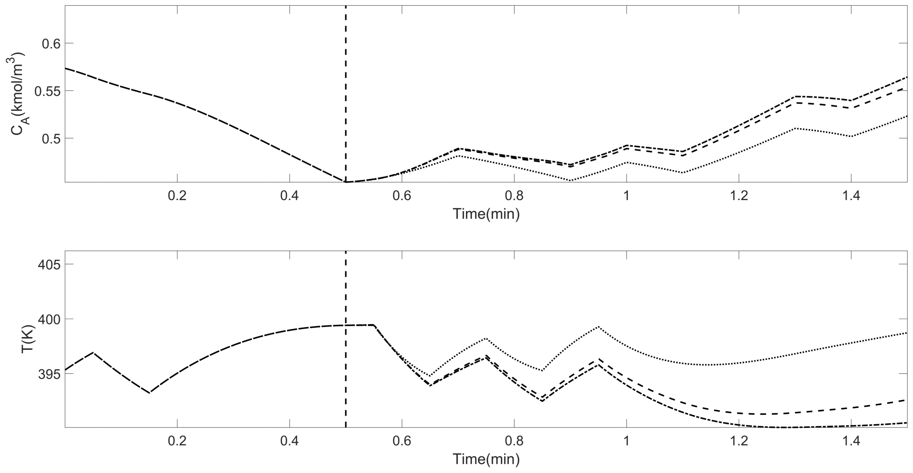
Next, the proposed Lyapunov-based EMPC (LEMPC) is implemented on the CSTR simulation example and compared to the LMPC implementation. The closed-loop results are presented in Figure 8, Figure 9, Figure 10 and Figure 11. Exploiting the flexibility of operation within a neighborhood of the origin, the LEMPC drives the system to a point on the border of that neighborhood, which happens to be the optimal operating point, instead of the nominal operating point. Figure 12 shows the comparison of the LEMPC and LMPC. As expected, the LEMPC achieves improved economic returns compared to the conventional MPC.
6. Conclusions
In this study, a novel data-driven MPC is developed that enables stabilization at nominally unstable equilibrium points. This LMPC is then utilized within an economic MPC formulation to yield a data driven EMPC formulation. The proposed approach is described and compared against a representative MPC, and shown to be able to provide improved closed-loop performance.
Acknowledgments
Financial support from the McMaster Advanced Control Consortium (MACC) is gratefully acknowledged.
Author Contributions
Masoud Kheradmandi as the lead author was the primary contributor, contributed to conceiving and designing of the framework, performed all the simulations and wrote the first draft of the manuscript, and made susbequent revisions. The advisor Prashant Mhaskar contributed to conceiving and designing of the framework, analyzing the data and revising the paper.
Conflicts of Interest
The authors declare no conflict of interest.
References
- Rawlings, J.B.; Mayne, D.Q. Model Predictive Control: Theory and Design; Nob Hill Publishing: Madison, Wisconsin, 2009. [Google Scholar]
- Mhaskar, P.; El-Farra, N.H.; Christofides, P.D. Predictive control of switched nonlinear systems with scheduled mode transitions. IEEE Trans. Autom. Control 2005, 50, 1670–1680. [Google Scholar] [CrossRef]
- Mahmood, M.; Mhaskar, P. Constrained control Lyapunov function based model predictive control design. Int. J. Robust Nonlinear Control 2014, 24, 374–388. [Google Scholar] [CrossRef]
- Angeli, D.; Amrit, R.; Rawlings, J.B. On average performance and stability of economic model predictive control. IEEE Trans. Autom. Control 2012, 57, 1615–1626. [Google Scholar] [CrossRef]
- Bayer, F.A.; Lorenzen, M.; Müller, M.A.; Allgöwer, F. Improving Performance in Robust Economic MPC Using Stochastic Information. IFAC-PapersOnLine 2015, 48, 410–415. [Google Scholar] [CrossRef]
- Liu, S.; Liu, J. Economic model predictive control with extended horizon. Automatica 2016, 73, 180–192. [Google Scholar] [CrossRef]
- Müller, M.A.; Angeli, D.; Allgöwer, F. Economic model predictive control with self-tuning terminal cost. Eur. J. Control 2013, 19, 408–416. [Google Scholar] [CrossRef]
- Golshan, M.; MacGregor, J.F.; Bruwer, M.J.; Mhaskar, P. Latent Variable Model Predictive Control (LV-MPC) for trajectory tracking in batch processes. J. Process Control 2010, 20, 538–550. [Google Scholar] [CrossRef]
- MacGregor, J.; Bruwer, M.; Miletic, I.; Cardin, M.; Liu, Z. Latent variable models and big data in the process industries. IFAC-PapersOnLine 2015, 48, 520–524. [Google Scholar] [CrossRef]
- Narasingam, A.; Siddhamshetty, P.; Kwon, J.S.I. Handling Spatial Heterogeneity in Reservoir Parameters Using Proper Orthogonal Decomposition Based Ensemble Kalman Filter for Model-Based Feedback Control of Hydraulic Fracturing. Ind. Eng. Chem. Res. 2018. [Google Scholar] [CrossRef]
- Narasingam, A.; Kwon, J.S.I. Development of local dynamic mode decomposition with control: Application to model predictive control of hydraulic fracturing. Comput. Chem. Eng. 2017, 106, 501–511. [Google Scholar] [CrossRef]
- Huang, B.; Kadali, R. Dynamic Modeling, Predictive Control and Performance Monitoring: A Data-Driven Subspace Approach; Springer: Berlin/Heidelberg, 2008. [Google Scholar]
- Li, W.; Han, Z.; Shah, S.L. Subspace identification for FDI in systems with non-uniformly sampled multirate data. Automatica 2006, 42, 619–627. [Google Scholar] [CrossRef]
- Hajizadeh, I.; Rashid, M.; Turksoy, K.; Samadi, S.; Feng, J.; Sevil, M.; Hobbs, N.; Lazaro, C.; Maloney, Z.; Littlejohn, E.; et al. Multivariable Recursive Subspace Identification with Application to Artificial Pancreas Systems. IFAC-PapersOnLine 2017, 50, 886–891. [Google Scholar] [CrossRef]
- Shah, S.L.; Patwardhan, R.; Huang, B. Multivariate controller performance analysis: methods, applications and challenges. In AICHE Symposium Series; American Institute of Chemical Engineers: New York, NY, USA, 1998; Volume 2002, pp. 190–207. [Google Scholar]
- Kheradmandi, M.; Mhaskar, P. Model predictive control with closed-loop re-identification. Comput. Chem. Eng. 2017, 109, 249–260. [Google Scholar] [CrossRef]
- Alanqar, A.; Ellis, M.; Christofides, P.D. Economic model predictive control of nonlinear process systems using empirical models. AIChE J. 2015, 61, 816–830. [Google Scholar] [CrossRef]
- Huang, B.; Ding, S.X.; Qin, S.J. Closed-loop subspace identification: An orthogonal projection approach. J. Process Control 2005, 15, 53–66. [Google Scholar] [CrossRef]
- Qin, S.J. An overview of subspace identification. Comput. Chem. Eng. 2006, 30, 1502–1513. [Google Scholar] [CrossRef]
- Wang, J.; Qin, S.J. A new subspace identification approach based on principal component analysis. J. Process Control 2002, 12, 841–855. [Google Scholar] [CrossRef]
- Mhaskar, P.; El-Farra, N.H.; Christofides, P.D. Stabilization of nonlinear systems with state and control constraints using Lyapunov-based predictive control. Syst. Control Lett. 2006, 55, 650–659. [Google Scholar] [CrossRef]
- Mayne, D.Q.; Rawlings, J.B.; Rao, C.V.; Scokaert, P.O. Constrained model predictive control: Stability and optimality. Automatica 2000, 36, 789–814. [Google Scholar] [CrossRef]
- Qin, S.J.; Ljung, L. Closed-loop subspace identification with innovation estimation. IFAC Proc. Vol. 2003, 36, 861–866. [Google Scholar] [CrossRef]
- Pannocchia, G.; Rawlings, J.B. Disturbance models for offset-free model-predictive control. AIChE J. 2003, 49, 426–437. [Google Scholar] [CrossRef]
- Ljung, L. System identification. In Signal Analysis and Prediction; Springer: Boston, MA, USA, 1998. [Google Scholar]
- Forssell, U.; Ljung, L. Closed-loop identification revisited. Automatica 1999, 35, 1215–1241. [Google Scholar] [CrossRef]
- Wallace, M.; Pon Kumar, S.S.; Mhaskar, P. Offset-free model predictive control with explicit performance specification. Ind. Eng. Chem. Res. 2016, 55, 995–1003. [Google Scholar] [CrossRef]
- Alanqar, A.; Durand, H.; Christofides, P.D. Fault-Tolerant Economic Model Predictive Control Using Error-Triggered Online Model Identification. Ind. Eng. Chem. Res. 2017, 56, 5652–5667. [Google Scholar] [CrossRef]
- Mahmood, M.; Mhaskar, P. Enhanced Stability Regions for Model Predictive Control of Nonlinear Process Systems. AIChE J. 2008, 54, 1487–1498. [Google Scholar] [CrossRef]
Figure 1.
Two-tier control strategy.
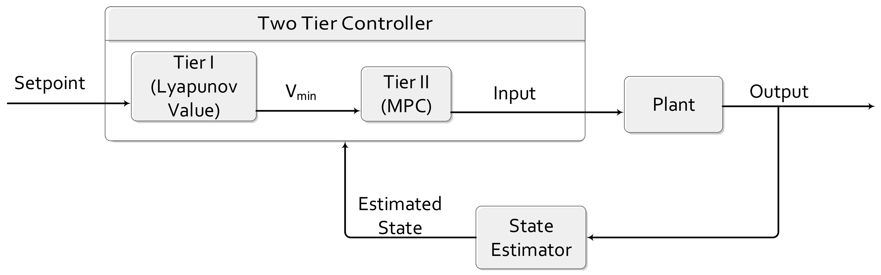
Figure 2.
Data driven model validation results: measured outputs (dash-dotted line), state and output estimates using the (linear time invariant) LTI model model from closed-loop data and identification (dashed line), state and output estimates using the LTI model from open-loop data and identification (dotted line), observer stopping point (vertical dashed line).

Figure 3.
Model validation data: manipulated inputs under a proportional–integral (PI) controller.

Figure 4.
Closed-loop profiles of the measured variables obtained from the proposed Lyapunov-based MPC (continuous line), MPC with horizon 1 (dash-dotted line), MPC with horizon 10 (dashed line), and MPC with horizon 1 and open-loop identification (narrow dash-dotted line) and set-point (dashed line).
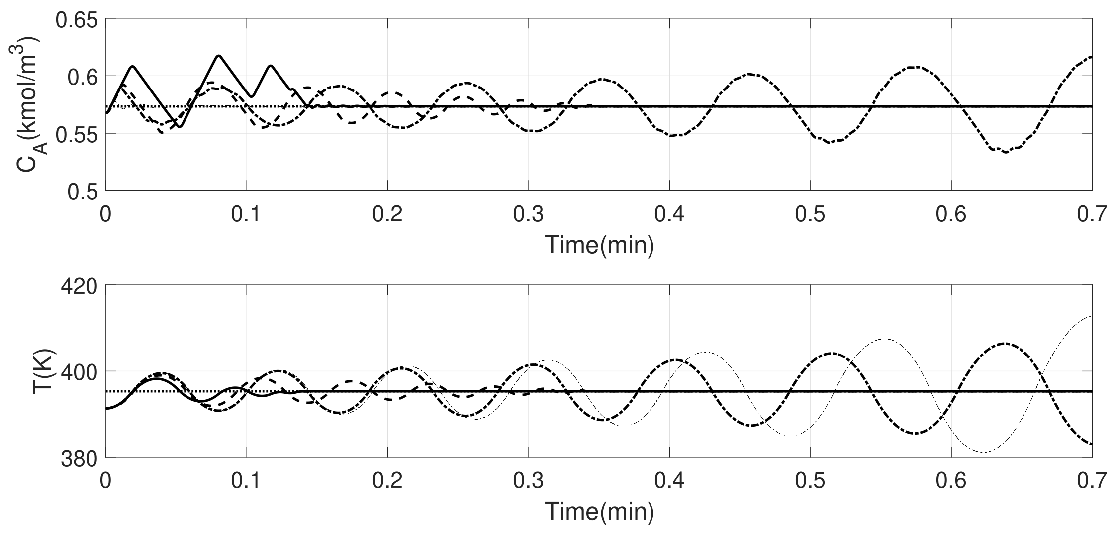
Figure 5.
Closed-loop profiles of the manipulated variables obtained from the proposed LMPC (continuous line), MPC with horizon 1 (dash-dotted line), MPC with horizon 1 and open-loop identification (narrow dash-dotted line) and MPC with horizon 10 (dashed line).
Figure 5.
Closed-loop profiles of the manipulated variables obtained from the proposed LMPC (continuous line), MPC with horizon 1 (dash-dotted line), MPC with horizon 1 and open-loop identification (narrow dash-dotted line) and MPC with horizon 10 (dashed line).

Figure 6.
Closed-loop profiles of the LTI model states obtained from the proposed LMPC (continuous line), MPC with horizon 1 (dash-dotted line) and MPC with horizon 10 (dashed line).
Figure 6.
Closed-loop profiles of the LTI model states obtained from the proposed LMPC (continuous line), MPC with horizon 1 (dash-dotted line) and MPC with horizon 10 (dashed line).
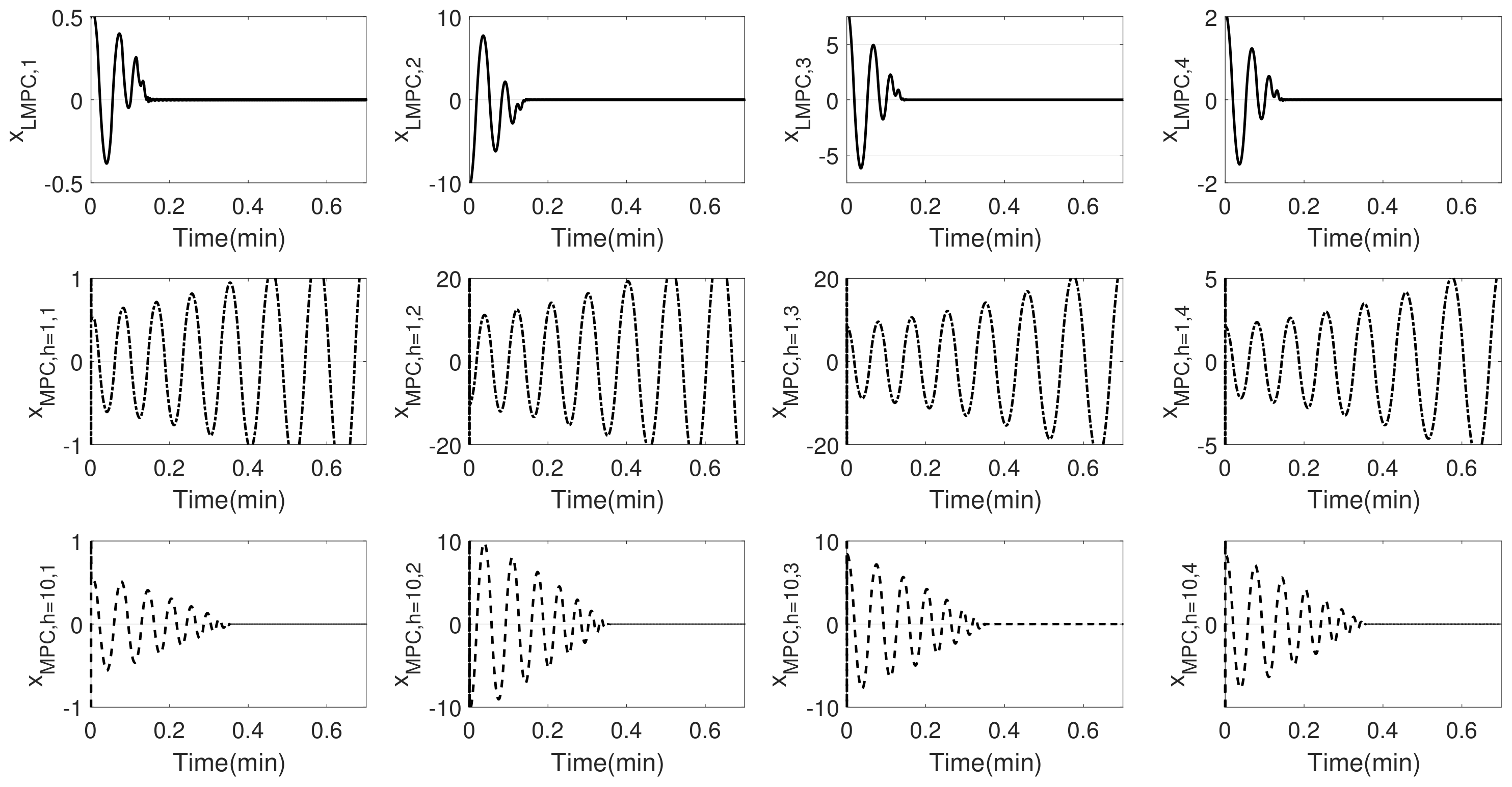
Figure 7.
Closed-loop Lyapunov function profiles obtained from the proposed LMPC (continuous line), MPC with horizon 1 (dash-dotted line) and MPC with horizon 10 (dashed line).
Figure 7.
Closed-loop Lyapunov function profiles obtained from the proposed LMPC (continuous line), MPC with horizon 1 (dash-dotted line) and MPC with horizon 10 (dashed line).
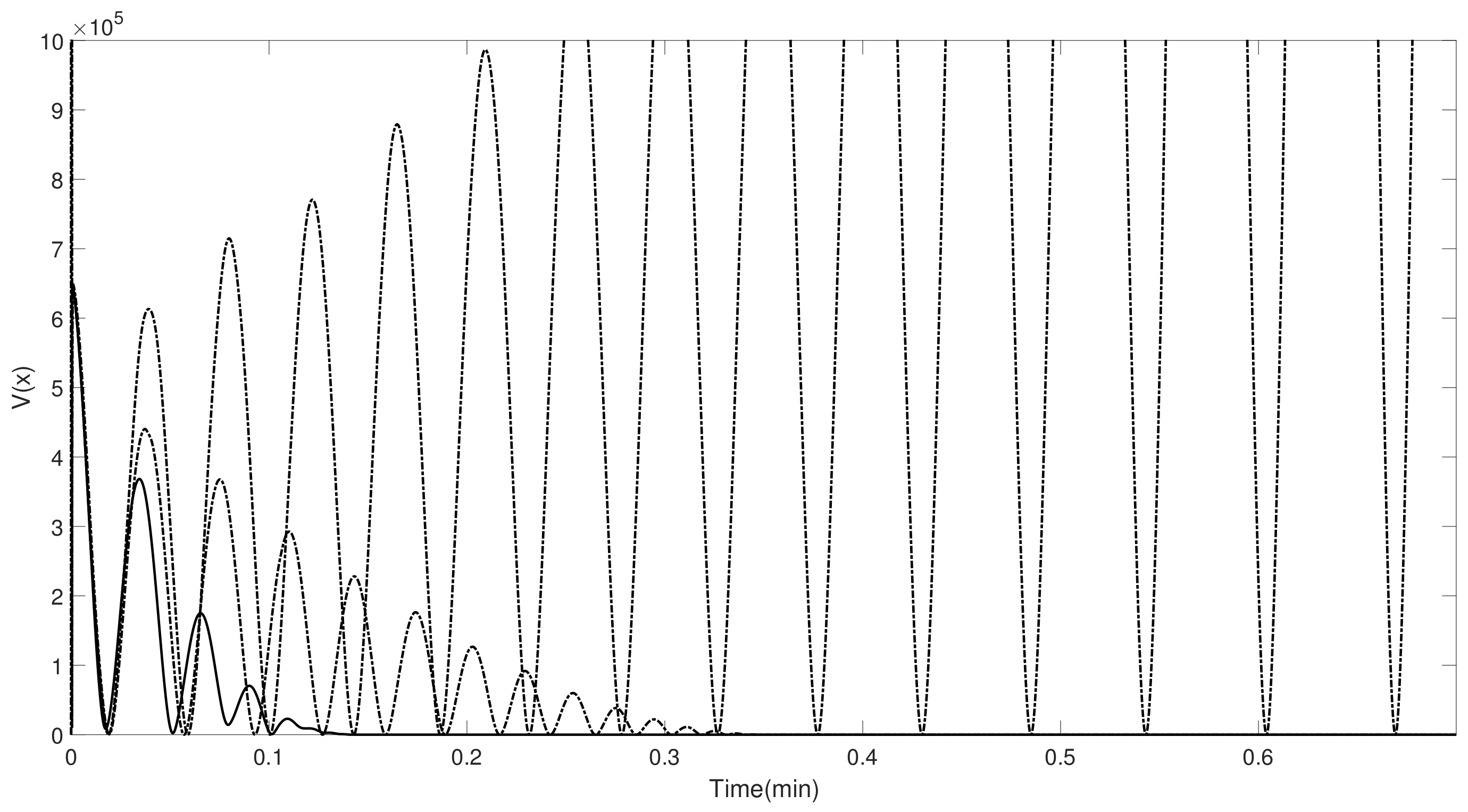
Figure 8.
Closed-loop profiles of the measured variables obtained from the proposed Lyapunov-based economic MPC (continuous line) and the nominal equilibrium point (dashed line).
Figure 8.
Closed-loop profiles of the measured variables obtained from the proposed Lyapunov-based economic MPC (continuous line) and the nominal equilibrium point (dashed line).
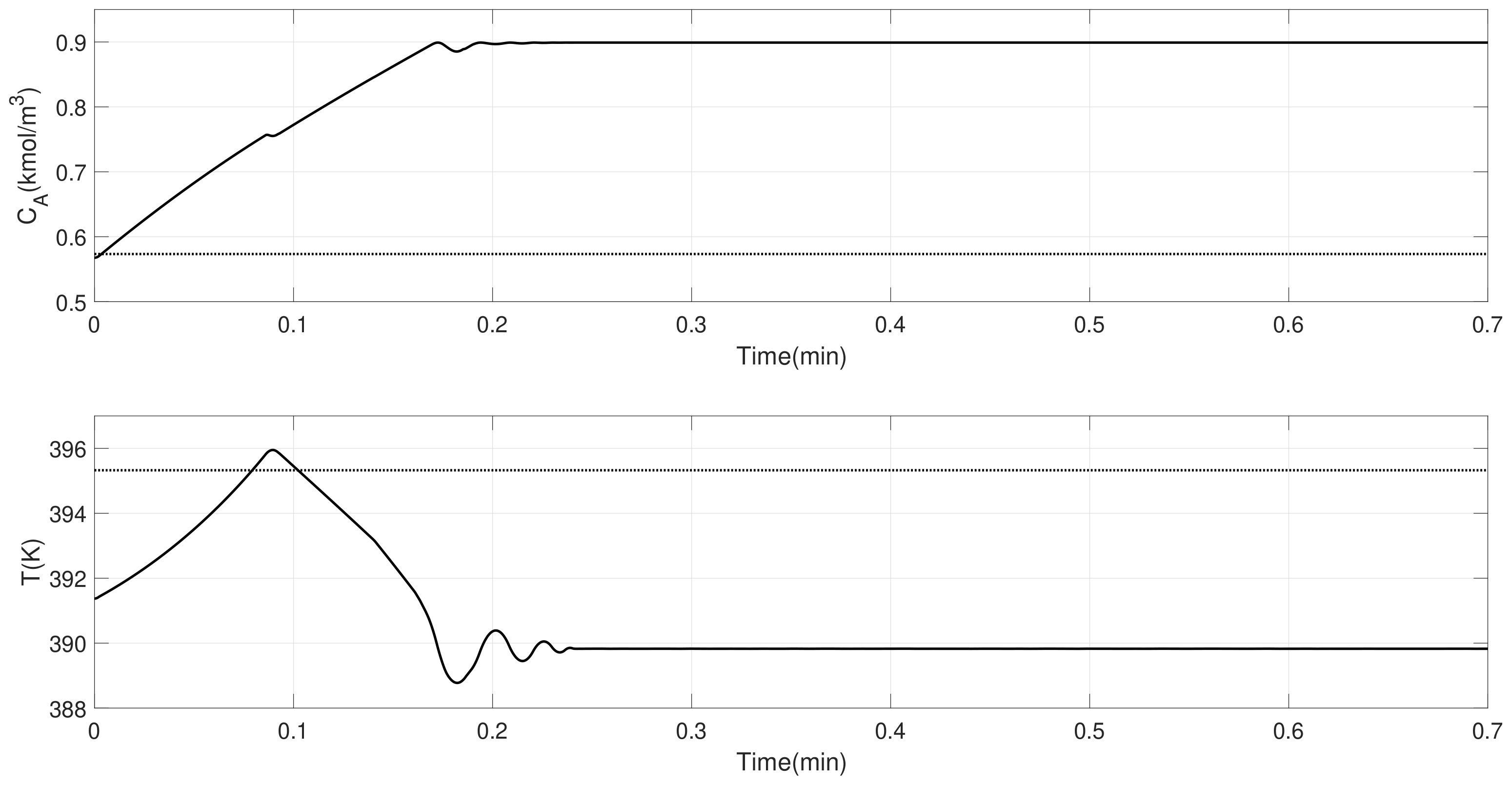
Figure 9.
Closed-loop profiles of the manipulated variables obtained from the proposed LEMPC (continuous line).
Figure 9.
Closed-loop profiles of the manipulated variables obtained from the proposed LEMPC (continuous line).
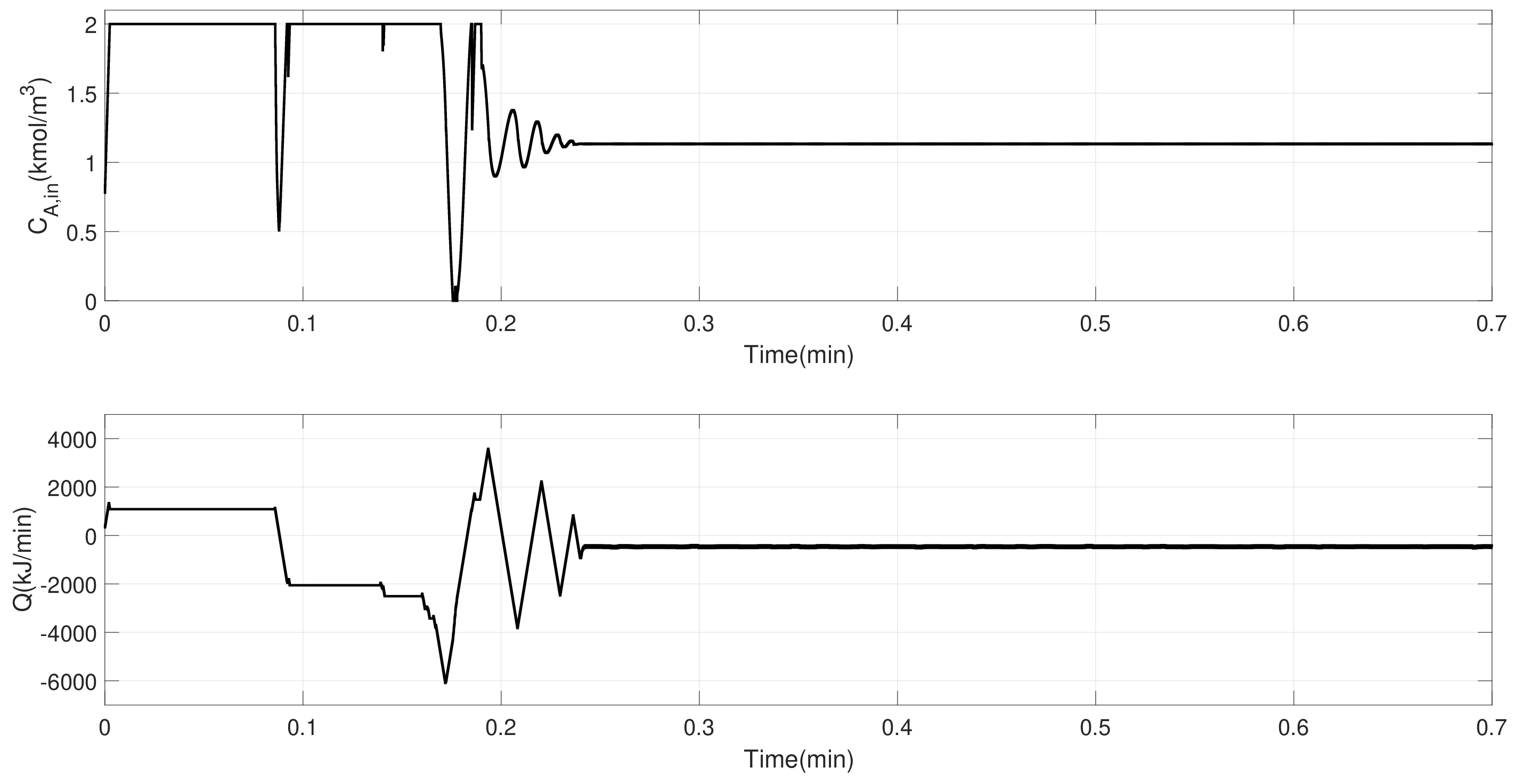
Figure 10.
Closed-loop profiles of the identified model states obtained from the proposed LEMPC (continuous line).
Figure 10.
Closed-loop profiles of the identified model states obtained from the proposed LEMPC (continuous line).
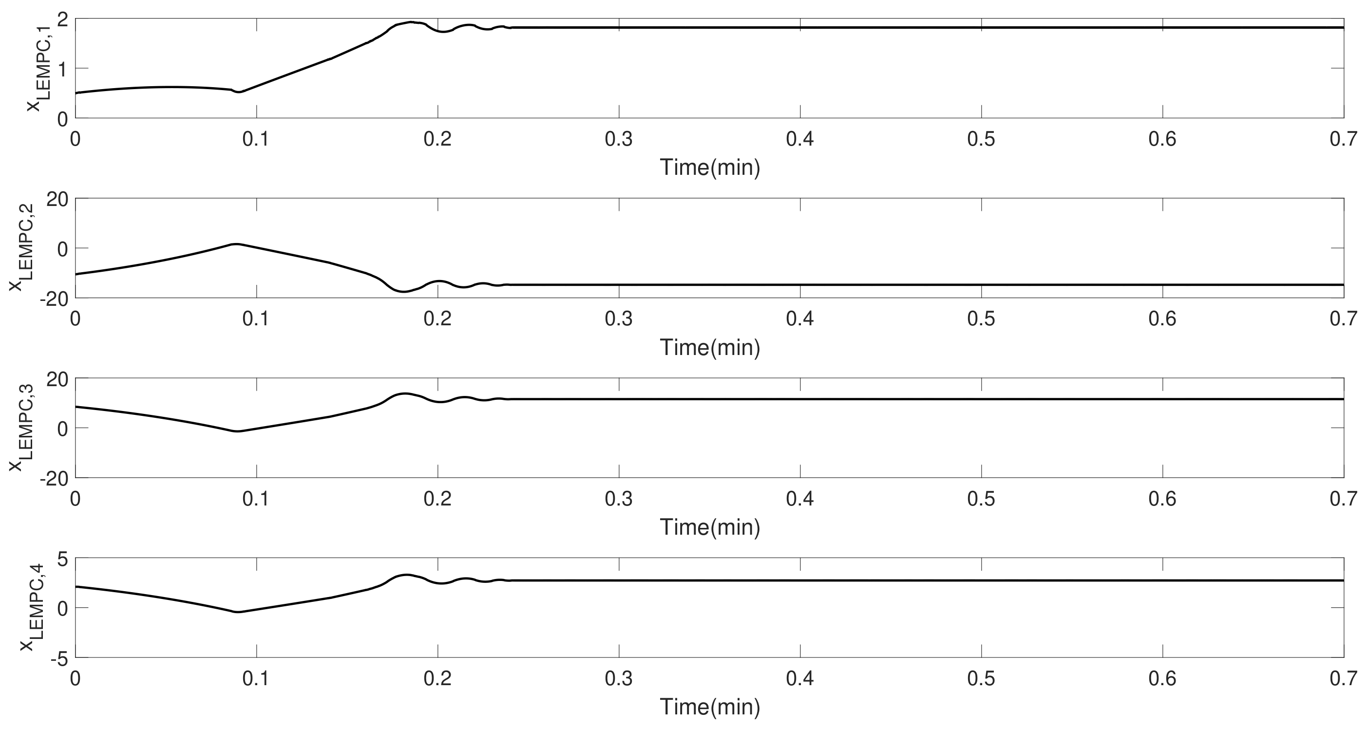
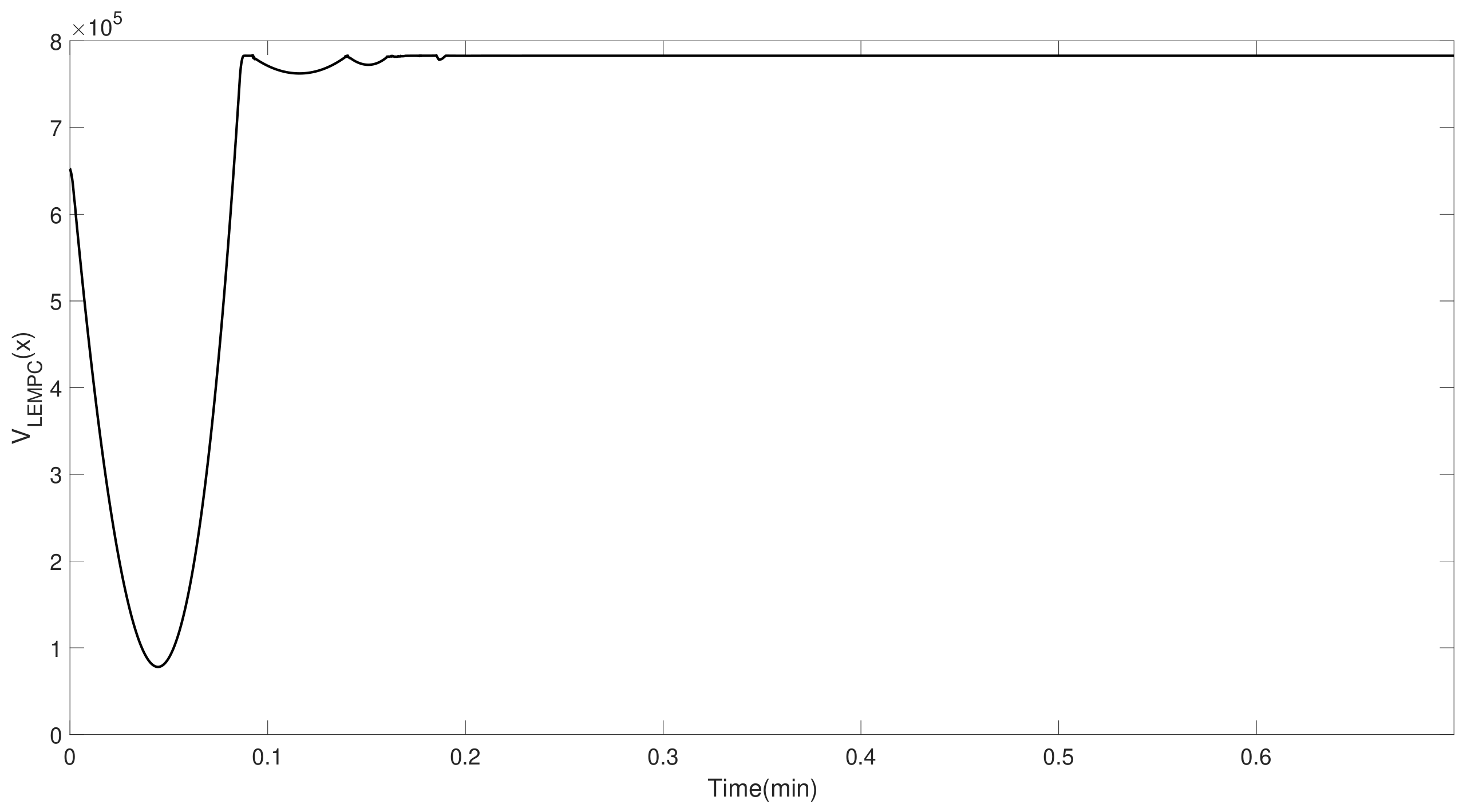
Figure 11.
Closed-loop Lyapunov function profiles obtained from the proposed LEMPC (continuous line). Note that the LEMPC drives the system to a point within the acceptable neighborhood of the origin.
Figure 11.
Closed-loop Lyapunov function profiles obtained from the proposed LEMPC (continuous line). Note that the LEMPC drives the system to a point within the acceptable neighborhood of the origin.

Figure 12.
A comparison of the economic cost between the LEMPC (continuous line) and LMPC (dotted line).
Figure 12.
A comparison of the economic cost between the LEMPC (continuous line) and LMPC (dotted line).

Table 1.
Variable and parameter description and values for the continuous stirred-tank reactor (CSTR) example.
Table 1.
Variable and parameter description and values for the continuous stirred-tank reactor (CSTR) example.
| Variable | Description | Unit | Value |
|---|---|---|---|
| Nominal Value of Concentration | |||
| Nominal Value of Reactor Temperature | K | 395 | |
| F | Flow Rate | ||
| V | Volume of the Reactor | ||
| Nominal Inlet Concentration | |||
| Pre-Exponential Constant | − | ||
| E | Activation Energy | ||
| R | Ideal Gas Constant | ||
| Inlet Temperature | K | ||
| Enthalpy of the Reaction | |||
| Fluid Density | |||
| Heat Capacity |
Table 2.
List of controllers parameters for the CSTR reactor.
| Variable | Value |
|---|---|
| min | |
| 0 | |
| 5 | |
| 1 | |
© 2018 by the authors. Licensee MDPI, Basel, Switzerland. This article is an open access article distributed under the terms and conditions of the Creative Commons Attribution (CC BY) license (http://creativecommons.org/licenses/by/4.0/).
Share and Cite
MDPI and ACS Style
Kheradmandi, M.; Mhaskar, P. Data Driven Economic Model Predictive Control. Mathematics 2018, 6, 51. https://doi.org/10.3390/math6040051
AMA Style
Kheradmandi M, Mhaskar P. Data Driven Economic Model Predictive Control. Mathematics. 2018; 6(4):51. https://doi.org/10.3390/math6040051
Chicago/Turabian StyleKheradmandi, Masoud, and Prashant Mhaskar. 2018. "Data Driven Economic Model Predictive Control" Mathematics 6, no. 4: 51. https://doi.org/10.3390/math6040051
Note that from the first issue of 2016, this journal uses article numbers instead of page numbers. See further details here.