A Novel Distributed Economic Model Predictive Control Approach for Building Air-Conditioning Systems in Microgrids


School of Chemical Engineering, University of New South Wales, Sydney, NSW 2052, Australia
*
Author to whom correspondence should be addressed.
†
Current address: School of Electrical & Electronic Engineering, Nanyang Technological University, 50 Nanyang Avenue, Singapore.
Mathematics 2018, 6(4), 60; https://doi.org/10.3390/math6040060
Submission received: 26 March 2018
/
Revised: 12 April 2018
/
Accepted: 13 April 2018
/
Published: 17 April 2018
(This article belongs to the Special Issue New Directions on Model Predictive Control)
Abstract
:With the penetration of grid-connected renewable energy generation, microgrids are facing stability and power quality problems caused by renewable intermittency. To alleviate such problems, demand side management (DSM) of responsive loads, such as building air-conditioning system (BACS), has been proposed and studied. In recent years, numerous control approaches have been published for proper management of single BACS. The majority of these approaches focus on either the control of BACS for attenuating power fluctuations in the grid or the operating cost minimization on behalf of the residents. These two control objectives are paramount for BACS control in microgrids and can be conflicting. As such, they should be considered together in control design. As individual buildings may have different owners/residents, it is natural to control different BACSs in an autonomous and self-interested manner to minimize the operational costs for the owners/residents. Unfortunately, such “selfish” operation can result in abrupt and large power fluctuations at the point of common coupling (PCC) of the microgrid due to lack of coordination. Consequently, the original objective of mitigating power fluctuations generated by renewable intermittency cannot be achieved. To minimize the operating costs of individual BACSs and simultaneously ensure desirable overall power flow at PCC, this paper proposes a novel distributed control framework based on the dissipativity theory. The proposed method achieves the objective of renewable intermittency mitigation through proper coordination of distributed BACS controllers and is scalable and computationally efficient. Simulation studies are carried out to illustrate the efficacy of the proposed control framework.
1. Introduction
In the past decade, electricity generation by using renewable energy resources, such as solar energy, becomes increasingly popular due to its capability of saving fossil fuels and reducing emissions. As a result, the number of grid-connected solar generation (SG) plants rises rapidly. One of the drawbacks of SG is the fluctuations in its output power caused by renewable intermittency. In practice, large and rapid output power oscillations are often experienced in SG plants, which may lead to bus voltage instability or even blackouts in the electric grid [1,2,3]. Such stability problems become far more significant in the microgrids, where high penetration of SG plants can be expected [4]. One of the widely accepted solutions to the aforementioned stability problems is to increase the operating reserve of electric grid. This includes the installation of extra generators, deployment of a large amount of battery energy storage systems (BESSs), and demand side management (DSM), etc. Obviously, large scale implementation of either extra generators or BESSs will introduce very high costs. In comparison, DSM utilizes the load shifting potential of end-users and does not require additional infrastructure. Thus, DSM is considered to be one of the most cost-effective methods for providing operating reserve to the grid [5,6].
Conceptually, DSM indicates the management of electrical loads to diminish undesirable fluctuations in power flow while satisfying customer requirements. Some electrical loads are controllable, including washing machines, air-conditioners and ventilation systems, etc. Among all these loads, air-conditioners typically consume a significant portion of energy. This is especially true for modern buildings that employ central air-conditioning systems. Statistically, nearly 40% of the world’s end-use electric energy is consumed by buildings and more than 50% of the building energy is used for ventilation and air-conditioning [7,8,9]. This shows that control of building air-conditioning systems (BACS) can be crucial for maintaining power balance in the grid, and the thermal capacity of buildings can be used as an effective tool for smoothing the power flow and shaving peak power in microgrids.
In recent years, model predictive control (MPC) has been investigated in the optimal management and operation of energy systems (including BACSs) [10,11,12,13,14,15,16,17]. For example, Maasoumy et al. [14] proposed an MPC approach to regulate building heating, ventilation and air-conditioning (HVAC) systems to offer an ancillary service to automatic generation control (AGC). The proposed method contributes to improving the accuracy of AGC in power systems. However, the operating costs of building HVAC systems and the scenarios of large scale power systems with SGs are not considered. In [15,16,17], researchers proposed other model based control methods to manipulate the aggregated demand of BACSs to compensate for the power fluctuations caused by SG units. These methods essentially increase the operating reserve of electric grids. Nevertheless, the associated operating costs of BACS are still not considered. In fact, the operating costs are one of the main concerns of building residents and must be taken into account in BACS control. From the perspective of building residents, the main control objective of BACSs should be the minimization of operating cost so that their electricity bills can be reduced. In [18], a hierarchical economic MPC framework based on the time-scale difference between HVAC and building thermal energy storage was developed to improve the total operation cost. In this work, distributed control is adopted since different buildings are usually subject to different energy demands and ownerships.
To study general situations in microgrids, dynamic electricity prices are employed in this paper for energy trading of distributed buildings with SGs and BACSs. Theoretically, dynamic prices are based on the current and predicted power supply/demand information that is available in the commonly used day-ahead market. Certainly, such dynamic “prices” can be either actual electricity prices for a microgrid with financially independent buildings (where the prices impact owners’ economic costs) or virtual prices for a microgrid owned by one organization such as a university or company campus (where the “prices” are used as a token for the coordination of energy consumption of different buildings). With respect to the dynamic prices, each individual BACS controller can minimize its operating cost economically through demand management. This mechanism encourages BACS controllers to shave peak power demand in the high price region and shift it to a low price region. However, if not appropriately coordinated, a positive feedback loop might be formed. In this case, the prediction of an increasing electricity price stimulates building controllers to purchase and use more energy at the current step to save the predicted future SG outputs for possible energy selling at higher prices. This subsequently results in a further boosted electricity price. The presence of such a mechanism can significantly deteriorate the collective power flow profile of all participated buildings in the microgrid. Under some extreme conditions, voltage instability might also be incurred. Therefore, the formulation of the aforementioned positive feedback loop must be avoided through appropriate coordination of different BACS controllers. Proper coordination of microgrid users is necessary to attenuate excessive energy trading behaviors effectively. Advanced control methods, such as process control techniques, can be applied in this scenario to improve system-wide stability and performance [10,13,19,20]. Although some articles are published on the coordination of distributed controllers for microgrid applications [21,22,23], their nature of achieving economic optimum at an aggregation level makes them computationally complicated and not scalable for large scale systems, such as microgrids. Thus, distributed control without online centralized optimization is a better solution to the aforementioned problem.
In this paper, a novel distributed economic MPC approach for BACS in microgrids is developed, based on the dissipativity theory. This approach allows individual BACS MPCs to minimize their own operational costs while attenuating the fluctuations of the total power demand and ensure microgrid level stability. To allow large scale implementation, the basic idea is to constrain the behaviors of BACS controllers with additional conditions to achieve the microgrid level performance and stability. In this work, such conditions are developed based on concept of dissipativity. Being an input and output property of dynamical systems [24,25], dissipativity was found useful for stability design for feedback systems (e.g., [26,27]) and was recently applied to develop plantwide interaction analysis and distributed control approaches (e.g., [28,29,30,31]). In this paper, microgrid-wide performance and stability are represented as microgrid dissipativity conditions that in turn are translated into the constraints that each BACS controller has to satisfy. To reduce the conservativeness of the dissipativity conditions, dynamic supply rates in Quadratic Difference Form (QdF) [32] are adopted in this approach, similar to [33]. Each BACS controller can optimize its own “selfish” economic objective based on the local information (e.g., the indoor temperature) and the electricity price, subject to the above discussed constraint, without iterative optimization or negotiations.
The remaining part of this paper is organized as follows: Section 2 introduces thermal modeling of buildings with AC and SG for microgrid applications. In Section 3, the effect of dynamic electricity price on energy trading in microgrids is discussed and an illustrative price scheme is provided. The dissipativity theory is briefly reviewed in Section 4. Subsequently, microgrid-wide dissipativity is analyzed and the proposed control framework is presented. Based on the general case of dynamic electricity price, simulations are carried out with the results presented in Section 5 to show the effectiveness of the proposed approach on improving collective performance of BACSs in microgrids. Finally, a conclusion is drawn in Section 6.
2. Buildings with Air-Conditioning and Solar Generation in Microgrids
2.1. Building Thermal Modeling
To effectively reduce the energy consumption of BACS without sacrificing the comfort of residents, thermal dynamics of buildings have to be studied. Therefore, a suitable building thermal model is necessary. In literature, a number of models are proposed to quantitatively evaluate building thermal dynamics [34,35,36,37,38]. Typically, three exogenous disturbances, including ambient temperature, solar irradiation and heat generated by internal electrical appliances, are adopted in these models and ground temperature is neglected [35]. The complexity of these models are basically dependent on their accuracy and the number of thermal zones considered in a building. It is noted that linear state space models are commonly used and found to be accurate enough [36,37,38]. In addition, the complexity of such models rises drastically with the increase of the number of building thermal zones [39]. Therefore, in real-time control applications, a reduced order model is usually desirable. Without loss of generality, a lumped parameter building thermal model [38] is employed in this paper as follows:
where the definitions and units of notations used in Equation (1) are given in Table 1. Noticeably, expressions and represent the solar radiation transferred through an external building envelop to heat up indoor air and interior walls, respectively. Considering the effect of shading, the usage of heat insulation materials in the envelop of most buildings and the heat transfer rate between air and wall, the values of and are chosen to be 0.02 and 0.0075 in this paper. It should be pointed out that the control framework to be presented in Section 4 can be applied with any building thermal model, including those more detailed models that consider the dynamics of each individual thermal zone.
2.2. Building with Air-Conditioning and Solar Generation
As mentioned before, modern buildings are usually equipped with automatically controlled air-conditioners (AC), which includes on/off type and inverter based variable frequency type. In most cases, the latter shows superior performance over the former even though it is more expensive [40]. According to some previous studies, the variable frequency air-conditioner (VFAC) can achieve significant energy savings and simultaneously provide better comfort level [40,41,42] compared to its on/off counterpart. This means the increased capital cost of VFAC can be readily paid back through the reduction of electricity bills. Consequently, nowadays, VFACs are widely used to replace the conventional on/off models [43]. In view of such circumstances, the VFAC, which is capable of continuously adjusting its output heating/cooling power, is assumed to be the default air-conditioner for buildings in this paper.
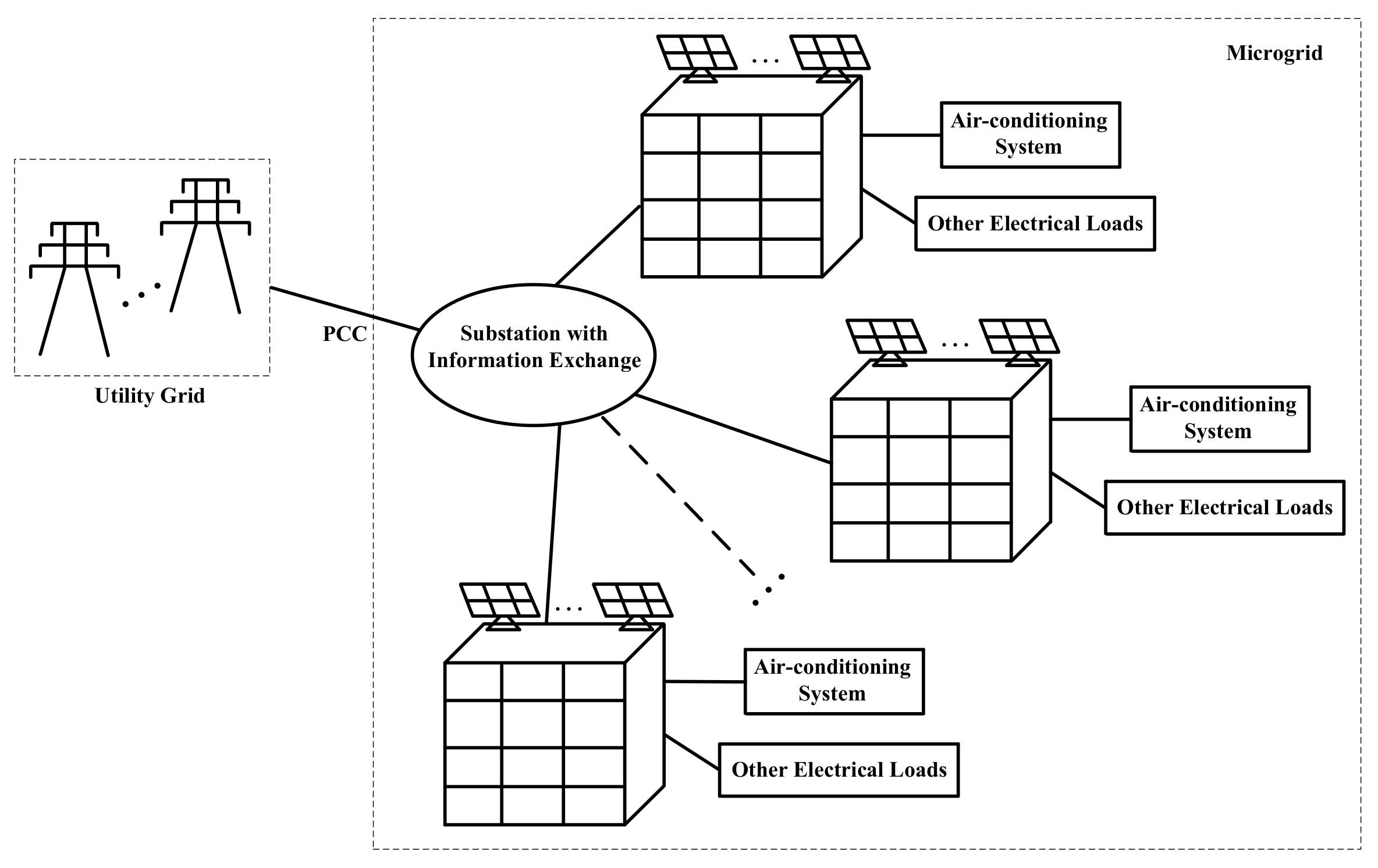
In the microgrids, it is common to install solar photovoltaic (PV) systems on the roof of buildings to reduce buildings’ energy dependency on the grid. In this way, many buildings can have their own clean energy sources to support loads or even sell surplus electric energy back to the grid. In order to describe a general situation, SG systems are assumed to be present in the buildings of microgrids in this work. Conceptually, the studied building system with AC and SG can be briefly depicted by Figure 1. Denote and as the power purchased from and sold to the microgrid by the building, respectively. Then, the power balance equation can be expressed as follows:
where and are defined as the power generated by SG plant and the power consumed by the other electrical loads (excluding AC system), respectively.
The output power of SG can be estimated/predicted from forecasted solar radiation and ambient temperature together with the technical specifications of the PV panels and the incremental conductance based maximum power point tracking algorithm [44].
2.3. State-Space Representation
The aim of controller is to maintenance the building’s indoor temperature with a certain range while dynamically adjusting the power demands within the microgrid to achieve better economy. Thus, the state variables x, output (or controlled) variables y, manipulated variables u and disturbance variables d can be chosen as follows:
respectively. The discrete-time state-space model of Equations (1)–(2) can be expressed in the following compact form:
where
with as the controller sampling period and as a identity matrix.
3. Electricity Price Policy for Energy Trading in Microgrids
There are research efforts on minimizing the operating costs of BACS based on the predictions of electricity price while respecting thermal comfort constraints [45,46,47,48]. Nonetheless, the attentions of these proposals are only based on static electricity price. Instead, the general case of dynamic electricity pricing, which varies with respect to real-time power supply and demand conditions, is not investigated. In practice, dynamic electricity prices are widely proposed for microgrid and smart grid applications [22,49,50,51] because they are effective tools for achieving power and financial balances. Furthermore, the existing proposals also neglect the effect of cost minimization by distributed BACS controllers on the overall power flow profile of microgrid. Actually, this effect is very important since the detrimental intermittent power fluctuations caused by renewable intermittency can be aggregated rather than mitigated if there is no coordination among distributed BACS controllers. The reason for such phenomenon is that buildings in one geographical area, such as a microgrid, are typically subject to the same electricity price and very similar weather conditions. As a consequence, simultaneous cost minimization of BACSs can lead to similar control actions, producing similar building power flow profiles even though there are some differences in the output of SGs installed on buildings.
It is acknowledged that a constant electricity price does not give customers incentives to change their load patterns, which can lead to supply issues in power systems during peak demand hours [9,52]. In addition, it implies that people who use electricity during off-peak hours are essentially subsidizing peak hour users [53]. Undoubtedly, such a price policy is undesirable for both the grid operator and the users. To effectively shave the peak of power demand, time-of-use (TOU) price policy is proposed and employed [47,54,55]. For example, a typical TOU price adopted by the state of New South Wales in Australia [54,55] is illustrated in Figure 2, from which it is seen that TOU electricity price varies with time periodically with large price difference between peak and non-peak hours. In this way, the shifting of electrical loads from peak hours to non-peak (off-peak or shoulder) hours can help reduce users’ electricity cost to a large extent. Therefore, TOU price policy motivates users to shift their electricity usage to low price regions.
Indeed, there are drawbacks of the existing TOU price policies. Firstly, researchers have pointed out that the ratio of peak to off-peak TOU prices has to be significant. Otherwise, the profile of user power demand will not change effectively [56]. Nevertheless, large price differences in different time intervals can result in higher overall cost for some users, and, thus, may not be preferable. Secondly, since the TOU price policy is static, dynamic supply and demand information cannot be reflected in the electricity price. Consequently, it is impossible for the electricity market to use price as an effective tool to affect power balance in the grid. In practice, dynamic electricity price has great potential to influence both the supply and demand to alleviate power imbalances in areas with high penetration of SG plants [49], such as microgrids. Theoretically, electric energy can be traded among users in microgrids with reasonable prices and this is beneficial for both grid operator and users. For the grid operator, electricity price can be regulated based on real-time supply and demand information to mitigate microgrid-wide power imbalance. Alternatively, for users in the microgrid, trading with the other users instead of the grid gives them the opportunity of getting a better electricity price. This contributes to reducing their overall cost. Therefore, dynamic electricity prices are promising for microgrid applications.
Of course, to implement dynamic electricity prices in the microgrid, energy trading between microgrid and utility grid (UG) is inevitable because power imbalances in microgrid have to be compensated by UG. As a result, the existing TOU price profile employed by UG must be considered. In general, the dynamic electricity prices should possess three features. First of all, they ought to be functions of the real-time power supply and demand in microgrid. Secondly, the users who buy energy should be charged at a price not higher than that of the UG and the users who sell energy should be paid at a price not lower than that of the UG. This feature motivates users to participate in energy trading activities. Thirdly, despite their nature of benefiting users, the dynamic electricity prices must guarantee that the microgrid can be financially self-sustained in its transactions with UG. In other words, the financial gain of microgrid through energy selling must be able to cover the financial loss of microgrid through energy buying. In theory, many pricing policies can satisfy the above features. One of the examples is
where and represent the electricity price charged on energy buyers and paid to energy sellers in microgrid, respectively, and (≥0) and (≤0) are the total electric power purchased from and sold to the microgrid by internal users, i.e.,
with and as the trading behaviors of individual users and M as the number of users. Notations and denote the electricity price charged on and paid to microgrid by UG when there are transactions between them. The values of and can be determined from Figure 2. Symbol is a user-defined constant in the range .
From Equation (6), it can be seen that
In both equations, the left-hand side represents financial gain/loss of microgrid’s trading with internal users and the right-hand side indicates financial gain/loss of microgrid’s trading with UG. Obviously, equivalence of the two sides implies zero financial gain/loss of microgrid. Consequently, by employing such a pricing policy, the microgrid serves as a non-profit information platform that facilitates energy trading among internal users. In practical applications, if certain operation and maintenance costs are associated with this information platform, a monthly service charge can be imposed on users. However, this service charge should be very low due to the large amount of users in microgrid and the marginal cost of running an information platform.
4. Dissipativity Based Distributed Control Framework
The distributed control diagram of building thermal systems in the microgrid is depicted by Figure 3, where and represent the i-th building and its corresponding controller. During each sampling period, individual controllers receive price information (both current and predicted purchasing/selling prices) from the energy trading unit, retrieve load profiles from historical data and measure building temperatures. Then, it calculates the control inputs by minimizing its economical cost and sending the power demand/supply information to the energy trading unit. The further price profile is generated by this centralized component based on the price scheme in Equation (6) and redistributed to individual controllers at the next time step.
As shown in our previous work [57], without proper coordination, the “selfish” nature of each economic MPC controller could generate excessive energy trading behaviors, which may cause undesirable oscillations. In this section, the dissipativity theory, which characterizes system behaviors from input–output trajectories, is employed to resolve this issue. The whole system in Figure 3 is treated as a network of dynamical interacted subsystems. Firstly, the dissipativity analysis is performed on each components, e.g., building thermal model, controller and energy trading unit. Then, a microgrid-wide supply rate is obtained by the linear combination of individual subsystems’ supply rates. Finally, a microgrid-wide dissipativity synthesis is performed offline and the online implementation involves solving distributed economic model predictive control (DEMPC) problems subject to additional dissipativity based coordination constraints.
4.1. Dissipativity and Dissipative Conditions
Consider a general discrete-time system expressed as follows:
where , and are defined as the state, input and output variables, respectively. Notation k denotes the k-th sampling instant. This system is said to be dissipative if there exists a positive semidefinite function defined on the state, called storage function, and a function defined on the input and output, which is known as supply rate, such that the following inequality holds [24]
Commonly, the following -type supply rate is used
where , and are parametric matrices. In general, the information of system gain is contained in and the phase relation is indicated by . For example, implies a system with bounded gain (with an system norm of ).
Since the -type supply rate only contains input and output information at the current sampling instant, i.e., and , it can be very conservative. The conservativeness of the dissipativity conditions can be reduced by introducing the concept of dynamic supply rate, e.g., in the quadratic differential form (QDF) [32], or the QdF for discrete time systems [58]. Such a dynamic supply rate is a function of the input and output trajectories and, consequently, captures more behavioral features of the system. An exemplary illustration of an n-th order QdF supply rate is
where , , , and are the input and output trajectories defined by:
where . By using the above notation, a QdF storage function can be derived as follows:
where , , . It is noted that zero vectors are concatenated with , and to extend the dimension of parametric matrix. With slight abuse of notations, we use and to denote the coefficient matrix of supply rate and storage function, i.e.,
Subsequently, the QdF-type dissipativity [33] can be defined as follows.
Definition 1.
System (9) is said to be dissipative with respect to the n-th order QdF-type supply rate if there exists n-th order QdF-type storage function satisfying the following dissipation inequality:
It is noted that the change of storage function is expressed as
4.2. Dissipativity Analysis of an Individual Building in the Microgrid
Assume that there are M buildings participating in the energy trading in microgrid and the i-th () building system is expressed as follows:
where variables and matrices are defined in a similar way as those in (3)–(5).
The dissipativity property of individual building thermal model can be obtained as follows.
Proposition 1.
System (18) is dissipative with supply rate , if there exists a storage function satisfying the following linear matrix inequalities (LMIs)
where
4.3. Dissipativity Based DEMPC
In this work, a DEMPC approach is developed to control each BACS as MPC implement cost functions that directly reflect the actual operational costs of air-conditioners and can deal with constraints easily. For the i-th building with AC and SG, the economic optimal control problem can be expressed as follows:
where is the vector of decision variable and N is the prediction horizon. In addition, the constraint inequalities indicate limits imposed by user comfort temperature zone , power distribution line limit and rating of air-conditioner .
Similar to [57], an additional dissipativity based constraint is added to individual DEMPC controllers to achieve microgrid-wide stability and performance. Since MPC is a static control law without any storage function, it could be very conservative to impose the dissipation inequality (16) to the DEMPC formulation (21). To solve this problem, the concept of dissipative trajectory, which is the integral version of (16), is adopted in this work:
Definition 2
([31]). An MPC controller with the supply rate is said to trace a dissipative trajectory if the following condition is satisfied:
4.4. Analysis of Dissipativity of Price Controller in Microgrid
The energy trading unit is a memoryless rational function of total power supply () and demand (). The dissipation inequality of the CPC can be expressed as follows:
where is the quadratic supply rate (QSR) matrix. The problem in (25) can be solved efficiently by the sum-of-squares (SOS) programming method.
Here is a brief introduction to the basic concept of SOS programming. Let be the set of all polynomials in x with real coefficients and
be the subset of containing the SOS polynomials. Finding a sum of squares polynomial is equivalent to determination of the existence of a positive semidefinite matrix Q such that
where is a vector of monomials. The SOS decomposition (27) can be efficiently and reliably achieved through semidefinite programming (SDP) [59]. In this paper, open source MATLAB toolbox YALMIP (version R20170921, Linkoping University, Linköping, Sweden) [60] and SDP solver SeDuMi (version 1.05R5, maintained by CORAL Lab, Department of Industrial and Systems Engineering, Lehigh University, Bethlehem, PA, USA) [61] are used for finding the Q matrix.
The following n-th order QdF supply rate (augment of QSR supply rate) can be written as
where the permutation matrix is defined by
4.5. Microgrid-Wide Dissipativity Synthesis
Let the independent variables for the networked system be partitioned into the following sets:
Then, the microgrid-wide supply rate, which is the linear combination of the supply rates of individual subsystems, distributed controllers and energy trading unit can be represented as
where and with permutation matrices satisfying
By imposing different constraints on the above microgrid-wide supply rate, we can achieve different performances of the collective behavior of all buildings. In practice, the UG operator mainly pays attention to the power flow at point of common coupling (PCC) depicted in Figure 1 because it directly affects the stability and power quality of UG. Instead, the power flows within the microgrid are usually not of concern on condition that the limits of power distribution lines are taken care of by distributed controllers.
In the context of microgrid with a high penetration of SG plants, desirable performances at PCC include: (1) reduced peak-to-peak amplitude of power flow profile; and (2) attenuated amplitude of rapid power flow fluctuations. To satisfy these two requirements, a frequency weighted microgrid-wide performance (34) is employed in this paper for the collective behavior of all buildings
where and are defined in (31) and is a frequency dependent weighting function utilized to penalize the mid to high frequency fluctuations of total power flow of all buildings and the excessive energy trading by individual buildings. An example of is
where the Kronecker operator ⊗ is defined by . The weighting function can be chosen as follows to attenuate the high frequency power fluctuations:
with coefficients , and K representing controller sampling period, time constants and attenuation gain, respectively. In addition, Ω is a linear transformation matrix that puts weightings on both the overall power flow at PCC and the net power flow of each individual building as interpreted by
In this paper, the weightings in (35) are normalized with unity weighting assigned to the overall power flow at PCC (i.e., ) and a small positive weighting of assigned to the net power flow of each building. Physically, this means that the penalty on the amplitude of high frequency power fluctuations is mainly imposed on the overall power flow, while the excessive energy trading behavior of each building is also constrained.
4.6. Distributed Control Design and Implmentation
The proposed dissipativity based DEMPC involves two steps:
- Off-line dissipativity synthesis: The dissipativity property for a given system is not unique. A system can have different supply rates that represent different aspects of the process dynamics (e.g., the gain and phase conditions). Therefore, dissipativity conditions for all subsystems including individual buildings, BACS controllers and the pricing controller that allow the required microgrid-wide stability and performance condition in (34) need to be found during the offline design step. This is done by solving LMIs in (19) for dissipativity conditions for buildings (corresponding to the building model in (18)), feasibility conditions for individual EMPC controllers in (24), the dissipativity condition for the pricing controller in (28), and the dissipativity condition representing the microgrid-wide stability and performance in (39) simultaneously. The outcome of this step is the dissipativity conditions (more specifically, the supply rates , and for the i-th controller) that individual EMPC controllers need to satisfy.
5. Simulation Results
To demonstrate the efficacy of the proposed control framework, a simulation model of microgrid consisting of eight buildings with AC and SG is developed. These buildings can be divided into four groups with each two buildings in one group sharing the same thermal parameters. Simulation studies are carried out based on the illustrative dynamic price scheme presented in Section 3. The data of power consumption by electrical appliances in buildings are downloaded from Australian Energy Market Operator (AEMO) [62] and the information of weather conditions, including ambient temperature and solar radiation, is obtained from the weather station of Murdoch University [63]. For the reference, profiles of the aforementioned data for one building are plotted in Figure 4. Furthermore, the values of thermal parameters for different types of buildings (with their definitions given in Table 1) are given in Table 2. In addition, an exemplary weighting function is designed by selecting , rad/h, rad/h, and . The controller sampling period is selected to be 10 min and the online computation time for individual DEMPC controller is less than 10 s, which is negligible. The small control latency is due to the non-iterative feature of the proposed approach.
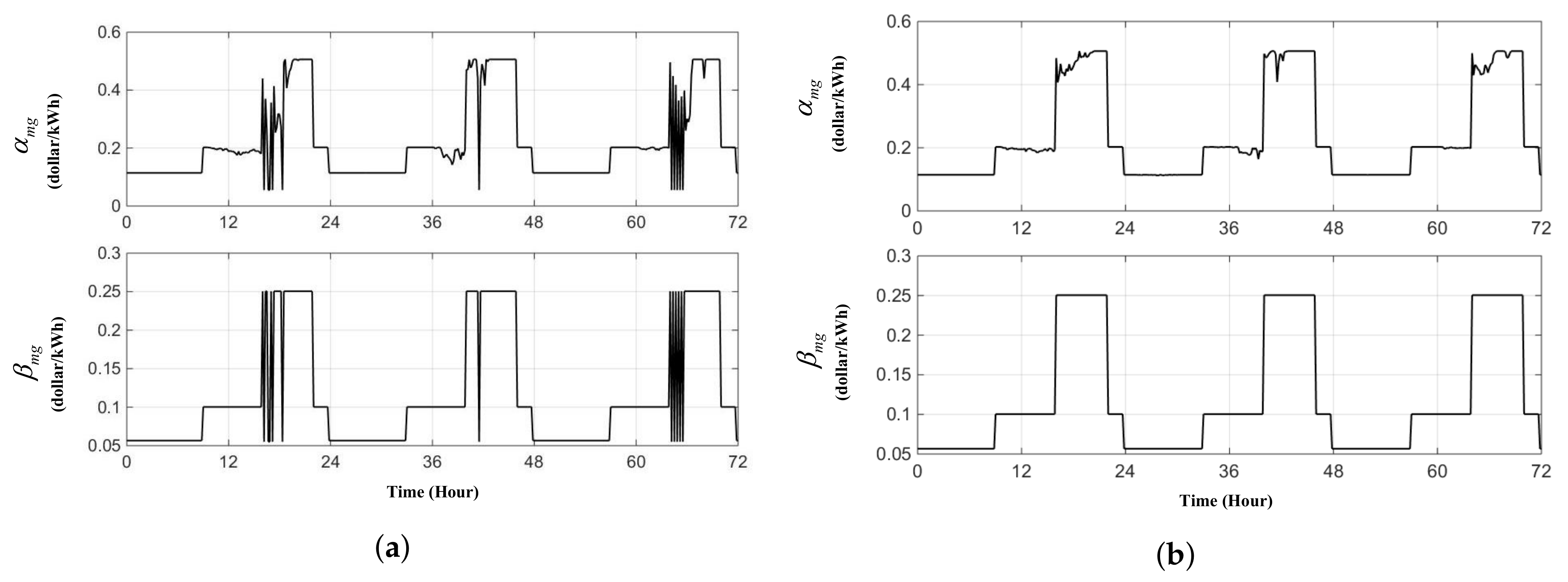
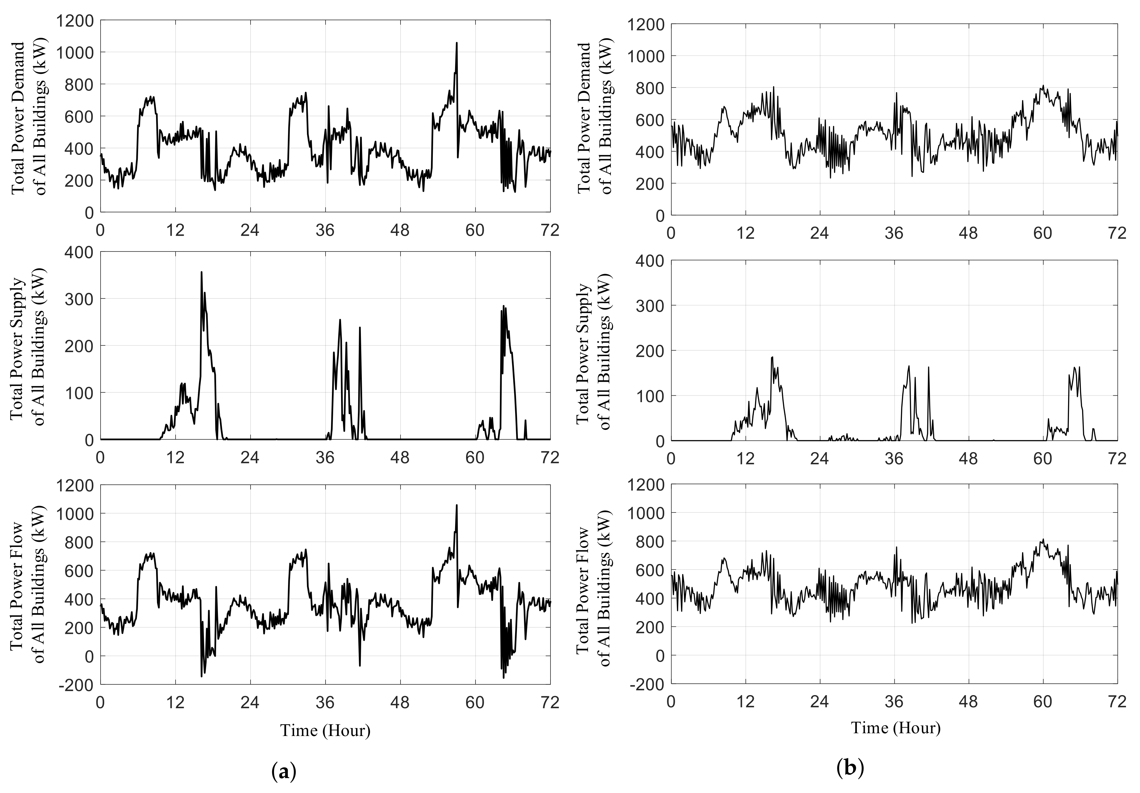
Firstly, the dynamic responses of different buildings are simulated by using distributed MPC as BACS controller without dissipativity based coordination (23). The results are given in Figure 5a and Figure 6a, from which high amplitude fluctuations are seen in both the dynamic electricity prices and the overall power flow of microgrid. This is caused by the “selfish” optimizations by distributed BACS controllers, which formulate a positive feedback loop in energy trading as analyzed in the Introduction.
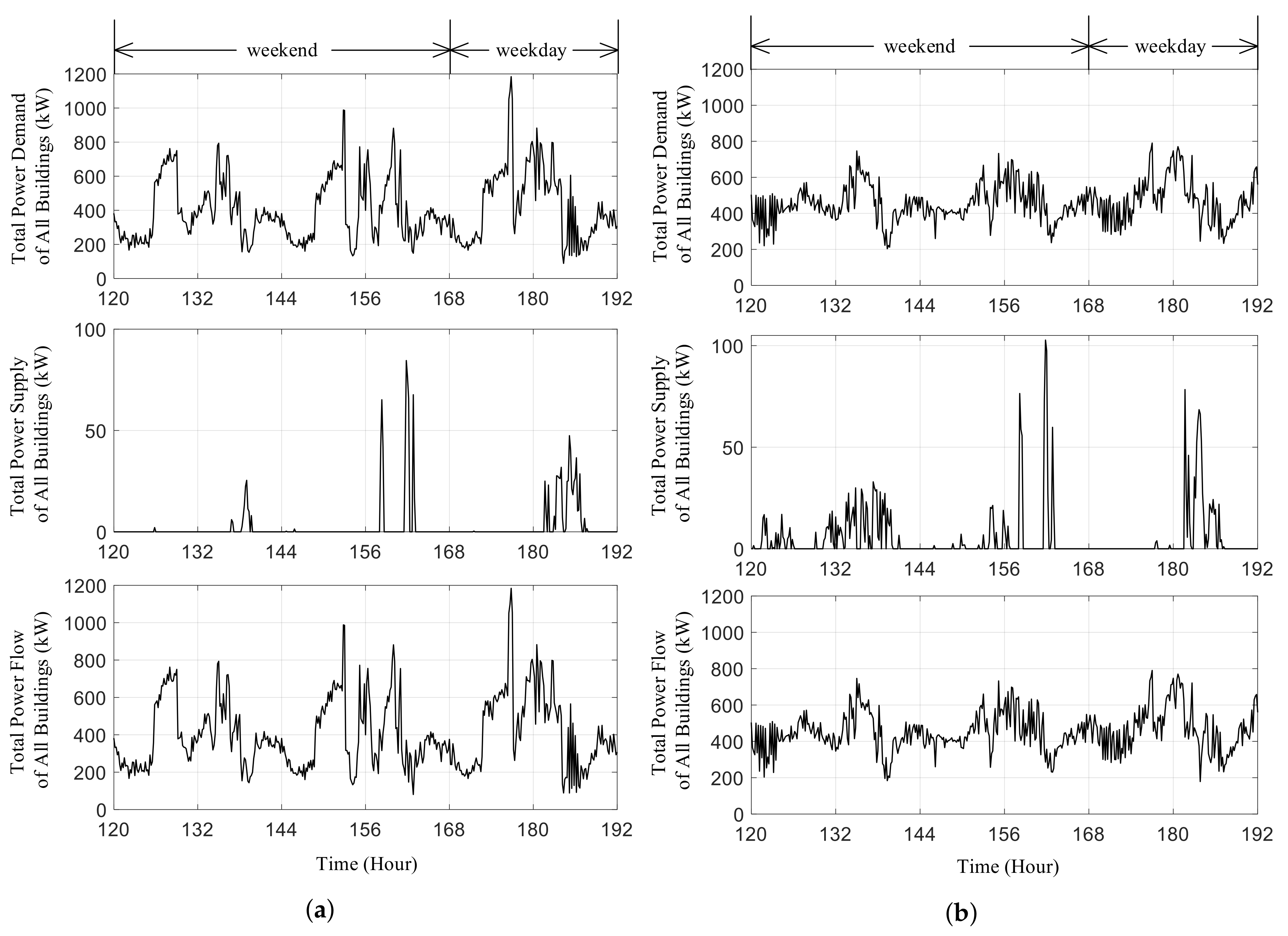
After implementing the dissipativity based coordination (23), which imposes constraints on the overall power flow of all participating buildings in the microgrid, comparative simulations are run under the same conditions of Figure 5a and Figure 6a. The corresponding results are shown in Figure 5b and Figure 6b. By comparing these four figures, it is seen that high amplitude fluctuations in electricity prices and the overall power flow are effectively attenuated, which implies successful mitigation of excessive energy trading of buildings. Moreover, from the third subplots of Figure 6, it is observable that the peak-to-peak amplitude of overall power flow is reduced by approximately 50% with the application of dissipativity based coordination. This means that coordination of distributed BACS controllers can reduce microgrid’s energy dependency on UG.
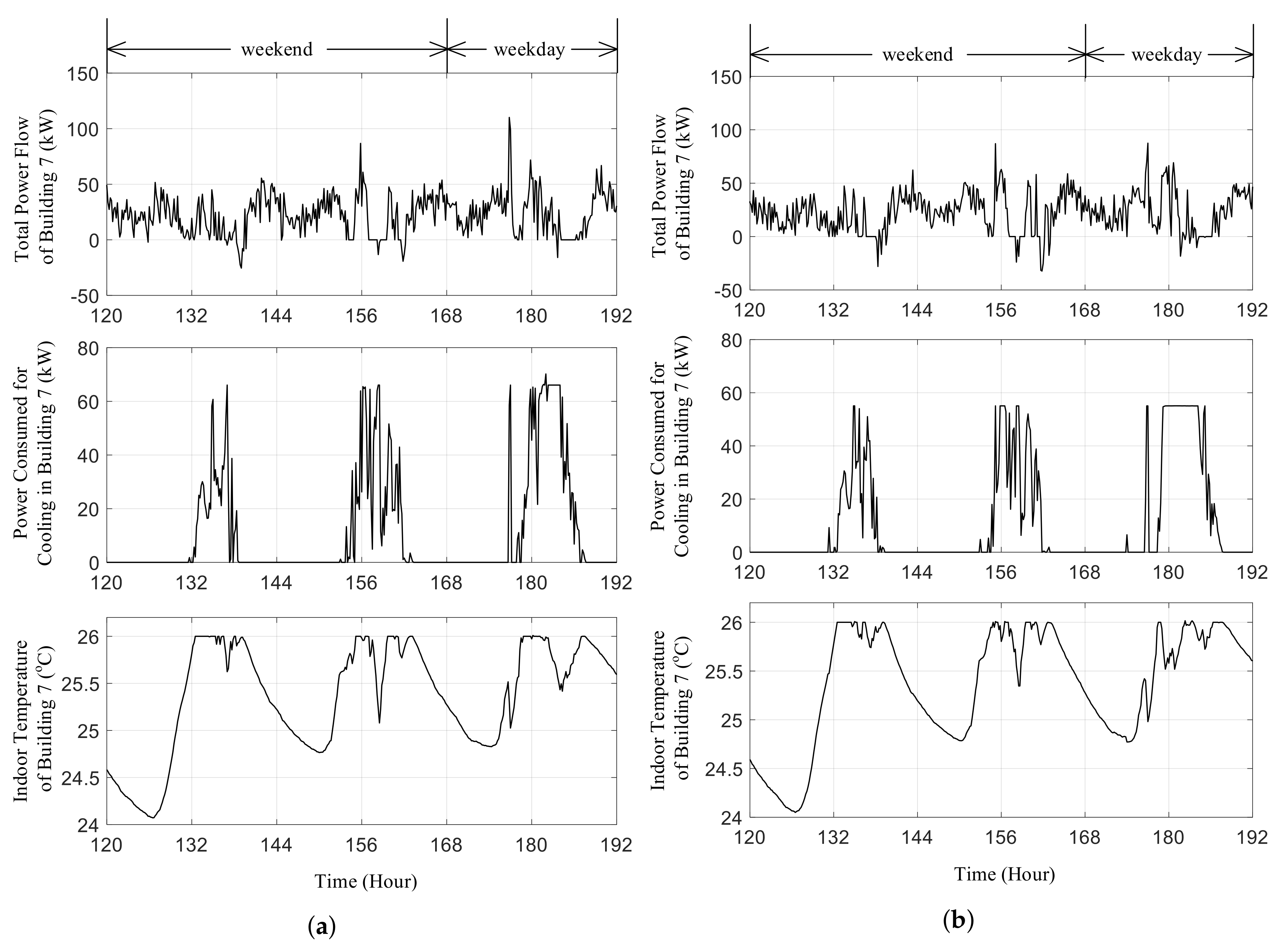
To investigate the impact of dissipativity based coordination on the response of individual buildings, corresponding simulation results are presented in Figure 7, from which it can be seen that the indoor temperature is kept within the required comfort zone and fluctuations in the total power flow and the consumption by AC of an individual building is also attenuated.
To further demonstrate the effectiveness of the proposed control framework, the responses of electricity prices and overall power flow profiles are simulated during the weekend. The corresponding results are given in Figure 8 and Figure 9, from which improvements on the damping of rapid fluctuations and peak-to-peak amplitude of power flow can also be seen in the responses with dissipativity based coordination.
6. Conclusions
This paper proposes a novel distributed control framework for the management of buildings with air-conditioners and SG in the context of microgrid. It allows the freedom of individually distributed building air-conditioner controllers in order to minimize their own operating costs, while achieving appropriate coordination among them to produce desirable overall power flow profile at the PCC. The effectiveness of the proposed control framework is demonstrated through simulation studies in comparison with conventional building air-conditioning control without coordination.
Acknowledgments
This work was supported by the Australian Research Council (Discovery Projects DP150103100).
Author Contributions
Xinan Zhang developed the main results, performed the simulation studies and prepared the initial draft of the paper. Ruigang Wang contributed to the distributed control theoretical developments. Jie Bao developed the dissipativity based distributed control idea, oversaw all aspects of the research and revised this manuscript.
Conflicts of Interest
The authors declare that they have no conflict of interest regarding the publication of the research article.
References
- Tonkoski, R.; Turcotte, D.; El-Fouly, T.H. Impact of high PV penetration on voltage profiles in residential neighborhoods. IEEE Trans. Sustain. Energy 2012, 3, 518–527. [Google Scholar] [CrossRef]
- Eftekharnejad, S.; Vittal, V.; Heydt, G.T.; Keel, B.; Loehr, J. Impact of increased penetration of photovoltaic generation on power systems. IEEE Trans. Power Syst. 2013, 28, 893–901. [Google Scholar] [CrossRef]
- Rahouma, A.; El-Azab, R.; Salib, A.; Amin, A.M. Frequency response of a large-scale grid-connected solar photovoltaic plant. In Proceedings of the SoutheastCon 2015, Fort Lauderdale, FL, USA, 9–12 April 2015; pp. 1–7. [Google Scholar]
- Wang, Y.; Zhang, P.; Li, W.; Xiao, W.; Abdollahi, A. Online overvoltage prevention control of photovoltaic generators in microgrids. IEEE Trans. Smart Grid 2012, 3, 2071–2078. [Google Scholar] [CrossRef]
- Jiang, B.; Muzhikyan, A.; Farid, A.M.; Youcef-Toumi, K. Demand side management in power grid enterprise control: A comparison of industrial & social welfare approaches. Appl. Energy 2017, 187, 833–846. [Google Scholar]
- Ramchurn, S.D.; Vytelingum, P.; Rogers, A.; Jennings, N. Agent-based control for decentralised demand side management in the smart grid. In Proceedings of the 10th International Conference on Autonomous Agents and Multiagent Systems, Taipei, Taiwan, 2–6 May 2011; Volume 1, pp. 5–12. [Google Scholar]
- Bellia, L.; Capozzoli, A.; Mazzei, P.; Minichiello, F. A comparison of HVAC systems for artwork conservation. Int. J. Refrig. 2007, 30, 1439–1451. [Google Scholar] [CrossRef]
- Lauro, F.; Moretti, F.; Capozzoli, A.; Panzieri, S. Model Predictive Control for Building Active Demand Response Systems. Energy Procedia 2015, 83, 494–503. [Google Scholar] [CrossRef]
- Xue, X.; Wang, S.; Yan, C.; Cui, B. A fast chiller power demand response control strategy for buildings connected to smart grid. Appl. Energy 2015, 137, 77–87. [Google Scholar] [CrossRef]
- Qi, W.; Liu, J.; Christofides, P.D. A distributed control framework for smart grid development: Energy/water system optimal operation and electric grid integration. J. Process Control 2011, 21, 1504–1516. [Google Scholar] [CrossRef]
- Qi, W.; Liu, J.; Chen, X.; Christofides, P.D. Supervisory predictive control of standalone wind/solar energy generation systems. IEEE Trans. Control Syst. Technol. 2011, 19, 199–207. [Google Scholar] [CrossRef]
- Qi, W.; Liu, J.; Christofides, P.D. Supervisory predictive control for long-term scheduling of an integrated wind/solar energy generation and water desalination system. IEEE Trans. Control Syst. Technol. 2012, 20, 504–512. [Google Scholar] [CrossRef]
- Qi, W.; Liu, J.; Christofides, P.D. Distributed supervisory predictive control of distributed wind and solar energy systems. IEEE Trans. Control Syst. Technol. 2013, 21, 504–512. [Google Scholar] [CrossRef]
- Maasoumy, M.; Sanandaji, B.M.; Sangiovanni-Vincentelli, A.; Poolla, K. Model predictive control of regulation services from commercial buildings to the smart grid. In Proceedings of the 2014 American Control Conference, Portland, OR, USA, 4–6 June 2014; pp. 2226–2233. [Google Scholar]
- Zhang, W.; Lian, J.; Chang, C.Y.; Kalsi, K. Aggregated modeling and control of air-conditioning loads for demand response. IEEE Trans. Power Syst. 2013, 28, 4655–4664. [Google Scholar] [CrossRef]
- Bashash, S.; Fathy, H.K. Modeling and control of aggregate air-conditioning loads for robust renewable power management. IEEE Trans. Control Syst. Technol. 2013, 21, 1318–1327. [Google Scholar] [CrossRef]
- Liu, M.; Shi, Y. Model predictive control of aggregated heterogeneous second-order thermostatically controlled loads for ancillary services. IEEE Trans. Power Syst. 2016, 31, 1963–1971. [Google Scholar] [CrossRef]
- Touretzky, C.R.; Baldea, M. Integrating scheduling and control for economic MPC of buildings with energy storage. J. Process Control 2014. [Google Scholar] [CrossRef]
- Soroush, M.; Chmielewski, D.J. Process systems opportunities in power generation, storage and distribution. Comput. Chem. Eng. 2013, 51, 86–95. [Google Scholar]
- Chen, X.; Heidarinejad, M.; Liu, J.; Christofides, P.D. Distributed economic MPC: Application to a nonlinear chemical process network. J. Process Control 2012, 22, 689–699. [Google Scholar]
- Vytelingum, P.; Voice, T.D.; Ramchurn, S.D.; Rogers, A.; Jennings, N.R. Agent-based micro-storage management for the smart grid. In Proceedings of the 9th International Conference on Autonomous Agents and Multiagent Systems, Toronto, ON, Canada, 10–14 May 2010; pp. 39–46. [Google Scholar]
- Maity, I.; Rao, S. Simulation and pricing mechanism analysis of a solar-powered electrical microgrid. IEEE Syst. J. 2010, 4, 275–284. [Google Scholar]
- Stephens, E.R.; Smith, D.B.; Mahanti, A. Game theoretic model predictive control for distributed energy demand-side management. IEEE Trans. Smart Grid 2015, 6, 1394–1402. [Google Scholar]
- Willems, J.C. Dissipative dynamical systems part I: General theory. Arch. Ration. Mech. Anal. 1972, 45, 321–351. [Google Scholar]
- Weiland, S.; Willems, J.C. Dissipative dynamical systems in a behavioral context. Math. Models Methods Appl. Sci. 1991, 1, 1–25. [Google Scholar]
- Hill, D.; Moylan, P. Stability Results for Nonlinear Feedback Systems. Automatica 1977, 13, 377–382. [Google Scholar]
- Moylan, P.; Hill, D. Stability criteria for large-scale systems. IEEE Trans. Autom. Control 1978, 23, 143–149. [Google Scholar]
- Xu, S.; Bao, J. Distributed control of plantwide chemical processes. J. Process Control 2009, 19, 1671–1687. [Google Scholar]
- Xu, S.; Bao, J. Control of chemical processes via output feedback controller networks. Ind. Eng. Chem. Res. 2010, 49, 7421–7445. [Google Scholar]
- Tippett, M.J.; Bao, J. Dissipativity based distributed control synthesis. J. Process Control 2013, 23, 755–766. [Google Scholar]
- Tippett, M.J.; Bao, J. Control of plant-wide systems using dynamic supply rates. Automatica 2014, 50, 44–52. [Google Scholar]
- Willems, J.; Trentelman, H. On quadratic differential forms. SIAM J. Control Optim. 1998, 36, 1703–1749. [Google Scholar]
- Tippett, M.J.; Bao, J. Distributed model predictive control based on dissipativity. AIChE J. 2013, 59, 787–804. [Google Scholar]
- Yu, Z.; Jia, L.; Murphy-Hoye, M.C.; Pratt, A.; Tong, L. Modeling and stochastic control for home energy management. IEEE Trans. Smart Grid 2013, 4, 2244–2255. [Google Scholar]
- Hazyuk, I.; Ghiaus, C.; Penhouet, D. Optimal temperature control of intermittently heated buildings using Model Predictive Control: Part I–Building modeling. Build. Environ. 2012, 51, 379–387. [Google Scholar]
- Ghosh, S.; Reece, S.; Rogers, A.; Roberts, S.; Malibari, A.; Jennings, N.R. Modeling the Thermal Dynamics of Buildings: A Latent-Force-Model-Based Approach. ACM Trans. Intell. Syst. Technol. 2015, 6, 7. [Google Scholar]
- Ma, Y.; Anderson, G.; Borrelli, F. A distributed predictive control approach to building temperature regulation. In Proceedings of the 2011 American Control Conference, San Francisco, CA, USA, 29 June–1 July 2011; pp. 2089–2094. [Google Scholar]
- Thavlov, A.; Bindner, H.W. Thermal models for intelligent heating of buildings. In Proceedings of the International Conference on Applied Energy, Suzhou, China, 5–8 July 2012. [Google Scholar]
- Haghighi, M.M. Controlling Energy-Efficient Buildings in the Context of Smart Grid: A Cyber Physical System Approach. Ph.D. Thesis, EECS Department, University of California, Berkeley, CA, USA, 2013. [Google Scholar]
- Nasution, H.; Hassan, M.N.W. Potential electricity savings by variable speed control of compressor for air-conditioning systems. Clean Technol. Environ. Policy 2006, 8, 105–111. [Google Scholar]
- Hunt, W.; Amarnath, A. Cooling Efficiency Comparison between Residential Variable Capacity and Single Speed Heat Pump. ASHRAE Trans. 2013, 119, Q1. [Google Scholar]
- Funami, K.; Nishi, H. Evaluation of power consumption and comfort using inverter control of air-conditioning. In Proceedings of the 37th Annual Conference on IEEE Industrial Electronics Society, Melbourne, VIC, Australia, 7–10 November 2011; pp. 3236–3241. [Google Scholar]
- Energy of the Environment Air Conditioners. 2016. Available online: http://www.energyrating.gov.au/products/space-heating-and-cooling/air-conditioners(Australian Government Equipment Energy Efficiency Program); (accessed on 24 April 2016).
- Lokanadham, M.; Bhaskar, K.V. Incremental conductance based maximum power point tracking (MPPT) for photovoltaic system. Int. J. Eng. Res. Appl. 2012, 2, 1420–1424. [Google Scholar]
- Ma, J.; Qin, S.J.; Salsbury, T. Experimental study of economic model predictive control in building energy systems. In Proceedings of the 2013 American Control Conference, Washington, DC, USA, 17–19 June 2013; pp. 3753–3758. [Google Scholar]
- Putta, V.; Zhu, G.; Kim, D.; Hu, J.; Braun, J. Comparative evaluation of model predictive control strategies for a building HVAC system. In Proceedings of the 2013 American Control Conference, Washington, DC, USA, 17–19 June 2013; pp. 3455–3460. [Google Scholar]
- Ma, J.; Qin, S.J.; Salsbury, T. Application of economic MPC to the energy and demand minimization of a commercial building. J. Process Control 2014, 24, 1282–1291. [Google Scholar]
- Brundage, M.P.; Chang, Q.; Li, Y.; Xiao, G.; Arinez, J. Energy efficiency management of an integrated serial production line and HVAC system. IEEE Trans. Autom. Sci. Eng. 2014, 11, 789–797. [Google Scholar]
- Braun, P.; Grüne, L.; Kellett, C.M.; Weller, S.R.; Worthmann, K. A real-time pricing scheme for residential energy systems using a market maker. In Proceedings of the 2015 5th Australian Control Conference (AUCC), Gold Coast, Australia, 5–6 November 2015; pp. 259–262. [Google Scholar]
- Ito, K. Nonlinear Pricing in Energy and Environmental Markets. Ph.D. Thesis, Agricultural & Resource Economics, University of California, Berkeley, CA, USA, 2011. [Google Scholar]
- Okawa, Y.; Namerikawa, T. Distributed dynamic pricing based on demand-supply balance and voltage phase difference in power grid. Control Theory Technol. 2015, 13, 90–100. [Google Scholar]
- Yang, L.; Dong, C.; Wan, C.J.; Ng, C.T. Electricity time-of-use tariff with consumer behavior consideration. Int. J. Prod. Econ. 2013, 146, 402–410. [Google Scholar]
- Rowlands, I.H.; Furst, I.M. The cost impacts of a mandatory move to time-of-use pricing on residential customers: An Ontario (Canada) case-study. Energy Effic. 2011, 4, 571–585. [Google Scholar]
- Matters, E. Feed-in Tariff for Grid-Connected Solar Power Systems. 2011. Available online: http://www.energymatters.com.au/rebates-incentives/feedintariff (accessed on 15 September 2015).
- Matters, E. Battery Storage And Solar Feed in Tariffs—State Of Play. 2015. Available online: http://www.energymatters.com.au/renewable-news/solar-fit-batteries-em5074/ (accessed on 15 September 2015).
- Muzmar, M.; Abdullah, M.; Hassan, M.; Hussin, F. Time of Use pricing for residential customers case of Malaysia. In Proceedings of the 2015 IEEE Student Conference on Research and Development (SCOReD), Kuala Lumpur, Malaysia, 13–14 December 2015; pp. 589–593. [Google Scholar]
- Zhang, X.; Bao, J.; Wang, R.; Zheng, C.; Skyllas-Kazacos, M. Dissipativity based distributed economic model predictive control for residential microgrids with renewable energy generation and battery energy storage. Renew. Energy 2017, 100, 18–34. [Google Scholar]
- Kojima, C.; Takaba, K. A generalized Lyapunov stability theorem for discrete-time systems based on quadratic difference forms. In Proceedings of the 44th IEEE Conference on Decision and Control, Seville, Spain, 15 December 2005; pp. 2911–2916. [Google Scholar]
- Parrilo, P.A. Structured Semidefinite Programs and Semialgebraic Geometry Methods in Robustness and Optimization. Ph.D. Thesis, California Institute of Technology, Pasadena, CA, USA, 2000. [Google Scholar]
- Löfberg, J. YALMIP: A toolbox for modeling and optimization in MATLAB. In Proceedings of the CACSD Conference, Taipei, Taiwan, 2–4 September 2004; pp. 284–289. [Google Scholar]
- Sturm, J.F. Using SeDuMi 1.02, a MATLAB toolbox for optimization over symmetric cones. Optim. Methods Softw. 1999, 11, 625–653. [Google Scholar] [CrossRef]
- Fan, S.; Hyndman, R.J. Short-term load forecasting based on a semi-parametric additive model. IEEE Trans. Power Syst. 2012, 27, 134–141. [Google Scholar]
- Station, M.U.W. 2017. Available online: http://wwwmet.murdoch.edu.au/downloads (accessed on 24 April 2016).
Figure 1.
Block diagram of buildings with air-conditioner (AC) and solar generation (SG) in microgrids.
Figure 1.
Block diagram of buildings with air-conditioner (AC) and solar generation (SG) in microgrids.

Figure 2.
Illustrative example of time-of-use (TOU) electricity price and solar feed-in tariff.
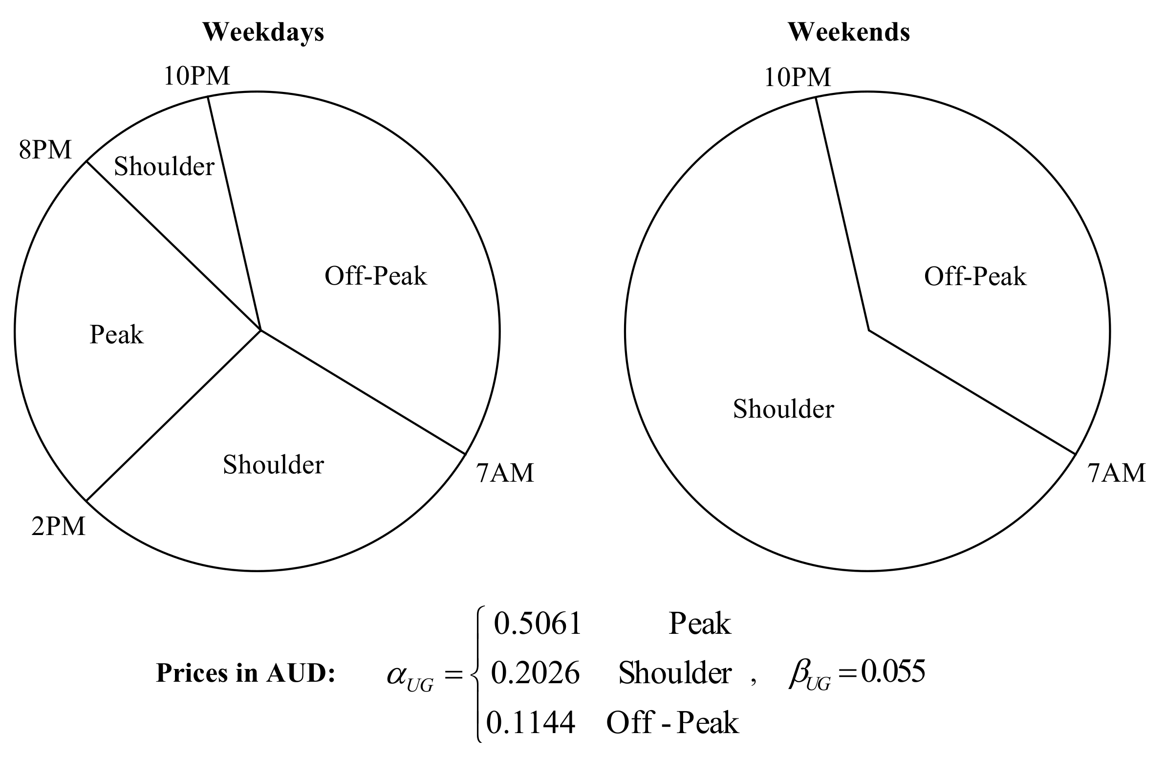
Figure 3.
Block diagram of signal flows of a controlled building thermal system.
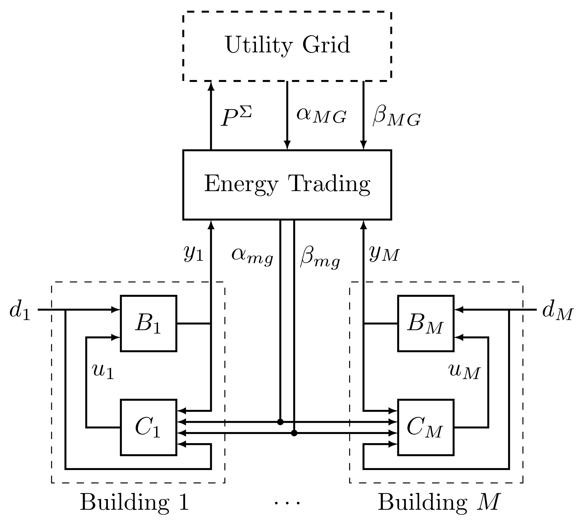
Figure 4.
Representative profiles of: (a) power consumption of electrical appliances (excluding building
air-conditioning systems (BACS)) in building 7 (kW); (b) ambient temperature of building 7 (°C); (c) solar radiation of buiding 1 (kW/m2).
Figure 4.
Representative profiles of: (a) power consumption of electrical appliances (excluding building
air-conditioning systems (BACS)) in building 7 (kW); (b) ambient temperature of building 7 (°C); (c) solar radiation of buiding 1 (kW/m2).
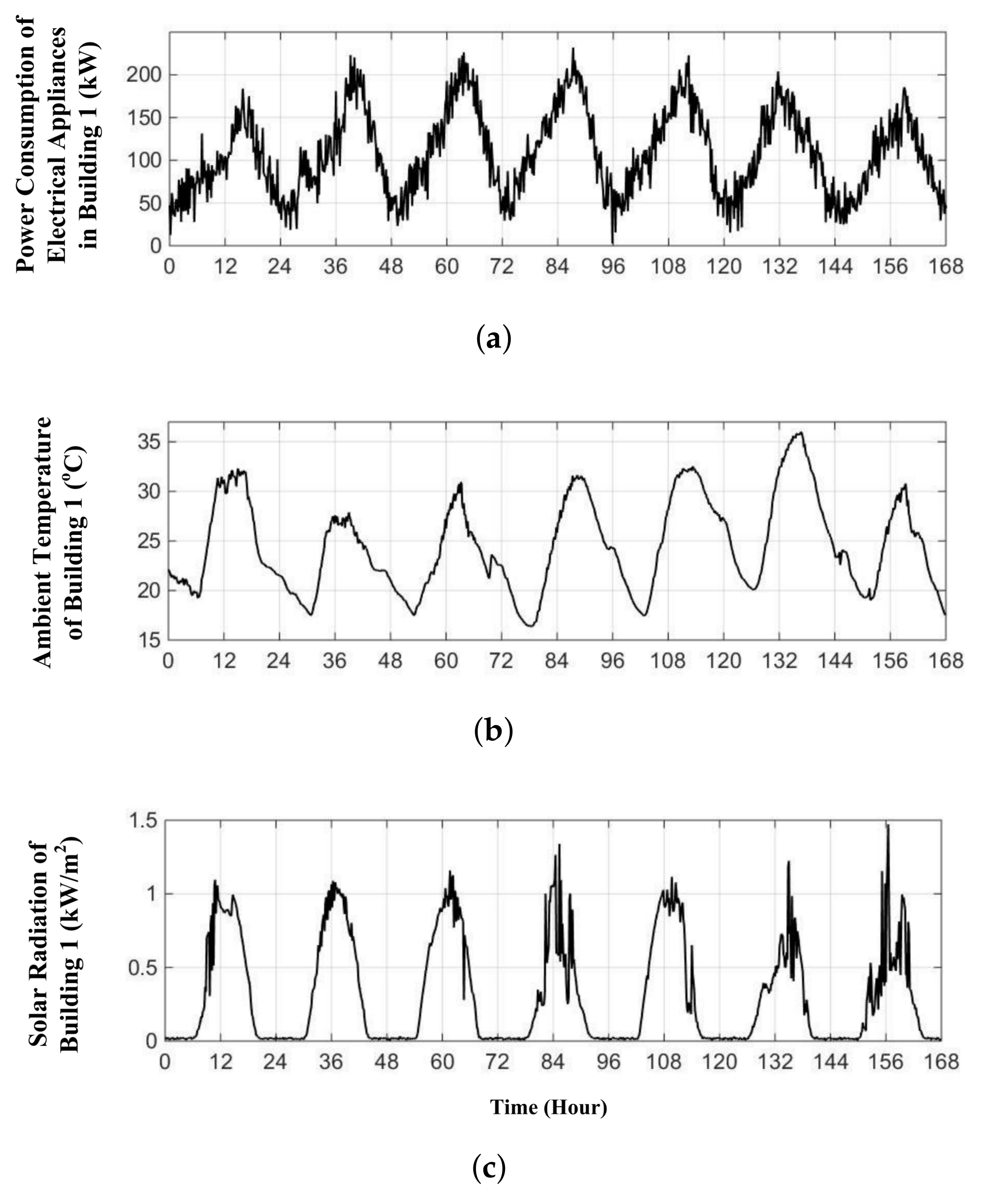
Figure 5.
Dynamic electricity price for energy trading: (a) with; (b) without dissipativity based coordination.
Figure 5.
Dynamic electricity price for energy trading: (a) with; (b) without dissipativity based coordination.

Figure 6.
Overall power flow profiles of all buildings: (a) without dissipativity based coordination; (b) with dissipativity based coordination.
Figure 6.
Overall power flow profiles of all buildings: (a) without dissipativity based coordination; (b) with dissipativity based coordination.

Figure 7.
Response of building 7: (a) without dissipativity based coordination; (b) with dissipativity based coordination.
Figure 7.
Response of building 7: (a) without dissipativity based coordination; (b) with dissipativity based coordination.

Figure 8.
Weekend dynamic electricity prices: (a) without dissipativity based coordination; (b) with dissipativity based coordination.
Figure 8.
Weekend dynamic electricity prices: (a) without dissipativity based coordination; (b) with dissipativity based coordination.
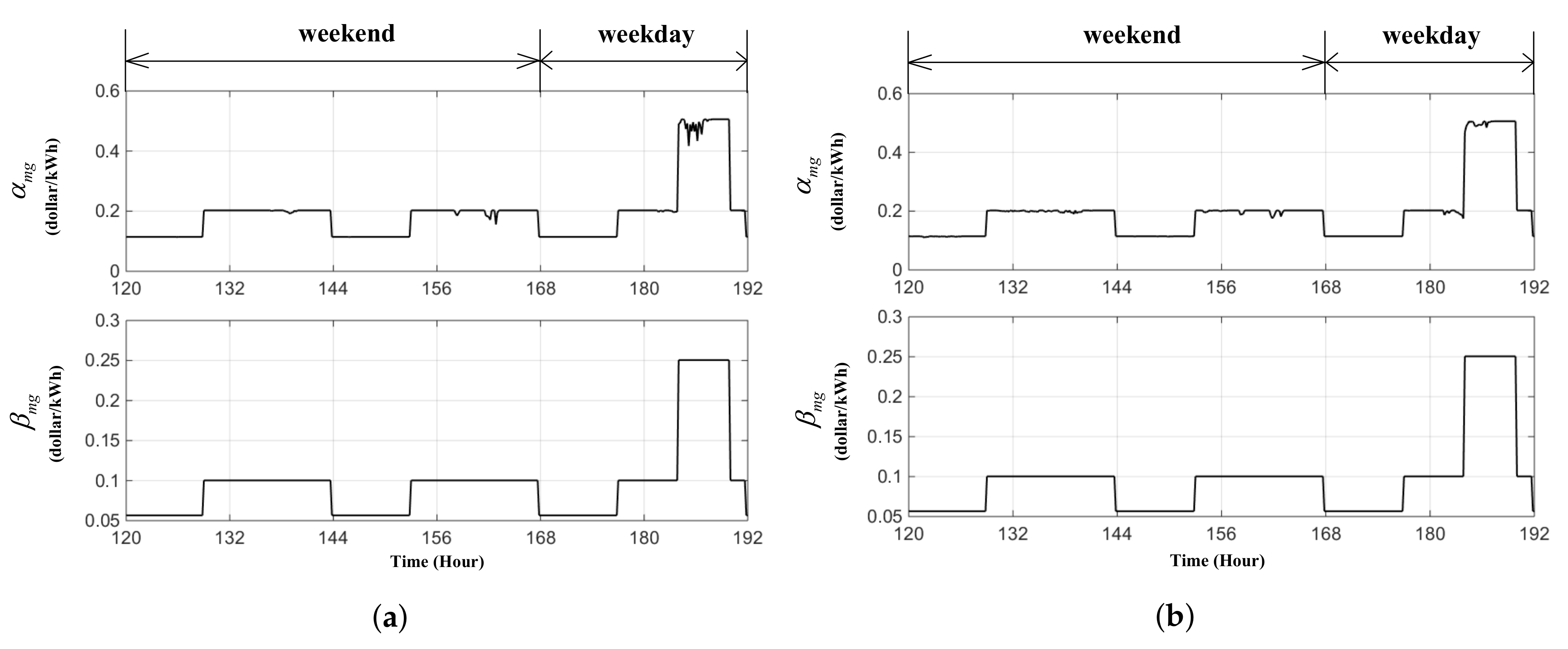
Figure 9.
Weekend overall power flow profiles of microgrid: (a) without dissipativity based coordination; (b) with dissipativity based coordination.
Figure 9.
Weekend overall power flow profiles of microgrid: (a) without dissipativity based coordination; (b) with dissipativity based coordination.


Table 1.
Variables in the thermal model.
| Variable | Definition | Unit |
|---|---|---|
| Temperature of building indoor air | C | |
| Temperature of building interior walls | C | |
| Temperature of building envelop | C | |
| Temperature of ambient environment | C | |
| Solar radiation | kW/m2 | |
| Heating power from air-conditioning system (positive) | kW | |
| Cooling power from air-conditioning system (negative) | kW | |
| Power consumption of indoor appliances (excluding AC system) | kW | |
| Fraction of heat generated from the operation of indoor appliances | ||
| Thermal resistance between indoor air and ambient environment | C/kW | |
| Thermal resistance between interior walls and indoor air | C/kW | |
| Thermal resistance between indoor air and building envelop | C/kW | |
| Thermal resistance between building envelop and ambient environment | C/kW | |
| Heat capacity of indoor air | kW/C | |
| Heat capacity of interior walls | kW/C | |
| Heat capacity of building envelop | kW/C | |
| A | Effective area of building envelop | m |
| Coefficient of solar radiation transferred through building envelop to heat up indoor air | ||
| Coefficient of solar radiation transferred through building envelop to heat up interior walls |
Table 2.
Values of thermal parameters for four types of buildings.
| Buildings | A | ||||||||||
|---|---|---|---|---|---|---|---|---|---|---|---|
| Type 1 | 3.26 | 0.21 | 0.132 | 0.0389 | 76.02 | 874.94 | 2767.1 | 0.02 | 0.0075 | 10500 | 0.1 |
| Type 2 | 4.22 | 0.22 | 0.142 | 0.133 | 37.04 | 337 | 1465.28 | 0.02 | 0.0075 | 3600 | 0.1 |
| Type 3 | 3.95 | 0.23 | 0.146 | 0.12 | 36.72 | 300 | 1302.5 | 0.02 | 0.0075 | 3200 | 0.1 |
| Type 4 | 3.54 | 0.2 | 0.144 | 0.142 | 32.85 | 312 | 1310 | 0.02 | 0.0075 | 3200 | 0.1 |
© 2018 by the authors. Licensee MDPI, Basel, Switzerland. This article is an open access article distributed under the terms and conditions of the Creative Commons Attribution (CC BY) license (http://creativecommons.org/licenses/by/4.0/).
Share and Cite
MDPI and ACS Style
Zhang, X.; Wang, R.; Bao, J. A Novel Distributed Economic Model Predictive Control Approach for Building Air-Conditioning Systems in Microgrids. Mathematics 2018, 6, 60. https://doi.org/10.3390/math6040060
AMA Style
Zhang X, Wang R, Bao J. A Novel Distributed Economic Model Predictive Control Approach for Building Air-Conditioning Systems in Microgrids. Mathematics. 2018; 6(4):60. https://doi.org/10.3390/math6040060
Chicago/Turabian StyleZhang, Xinan, Ruigang Wang, and Jie Bao. 2018. "A Novel Distributed Economic Model Predictive Control Approach for Building Air-Conditioning Systems in Microgrids" Mathematics 6, no. 4: 60. https://doi.org/10.3390/math6040060
Note that from the first issue of 2016, this journal uses article numbers instead of page numbers. See further details here.