Prey–Predator Models with Variable Carrying Capacity

Department of Mathematics and Statistics, College of Science, Sultan Qaboos University, Muscat 123, Oman
*
Author to whom correspondence should be addressed.
Mathematics 2018, 6(6), 102; https://doi.org/10.3390/math6060102
Submission received: 8 April 2018
/
Revised: 12 June 2018
/
Accepted: 13 June 2018
/
Published: 15 June 2018
Abstract
:Prey–predator models with variable carrying capacity are proposed. These models are more realistic in modeling population dynamics in an environment that undergoes changes. In particular, prey–predator models with Holling type I and type II functional responses, incorporating the idea of a variable carrying capacity, are considered. The carrying capacity is modeled by a logistic equation that increases sigmoidally between an initial value (a lower bound for the carrying capacity) and a final value (an upper bound for the carrying capacity). In order to examine the effect of the variable carrying capacity on the prey–predator dynamics, the two models were analyzed qualitatively using stability analysis and numerical solutions for the prey, and the predator population densities were obtained. Results on global stability and Hopf bifurcation of certain equilibrium points have been also presented. Additionally, the effect of other model parameters on the prey–predator dynamics has been examined. In particular, results on the effect of the handling parameter and the predator’s death rate, which has been taken to be the bifurcation parameter, are presented.
1. Introduction
Prey–predator dynamic is an essential tool in mathematical ecology, specifically for our understanding of interacting populations in the natural environment. This relationship will continue to be one of the dominant themes in both ecology and mathematical ecology due to its universal existence and importance. These problems may appear to be mathematically simple at first sight. However, they are, in fact, often very challenging and complicated. Moreover, although much progress has been made to the prey–predator theory in the last 40 years, many long standing mathematical and ecological problems remain open, such as modeling transient dynamics, environmental variability, complex ecological networks, and biodiversity extrapolation techniques [1]. All populations are affected by changes in their environment; therefore, there is a need to treat the carrying capacity as a system variable (i.e., function of time) in order to model population dynamics in an environment that undergoes changes [2]. In particular, in resource management, where the carrying capacity is often assumed to be constant and unchanging [3]. Many efforts to predict the world’s carrying capacity, the maximum sustainable population, are based on this assumption [4]. However, technological developments have raised crop yields, allowing a greater population to be supported by a smaller land area [5]. Thus, for the human population, a constant carrying capacity is not realistic [6]. Similarly, in nature, the inherent variability of natural systems [7] means that assuming an unchanging carrying capacity fails to adequately represent the environment.
Meyer et al. [8] proposed the carrying capacity to be modeled by a logistic equation that increases sigmoidally between an initial value and a final value . They studied the effect of this dynamic carrying capacity on the trajectories of simple growth models, and they use the new model to re-analyze two actual cases of the growth of human populations; English and Japanese examples with two pulses, or one change in limit, appear to verify their model.
A periodic form of carrying capacity has also been considered. For example, Shepherd et al. [9] has considered the following expression for the carrying capacity
where and are positive constants such that , ensuring the positive of , and is small and positive.
They demonstrated that, when the carrying capacity varies slowly with time, a multiple time scale analysis leads to approximate closed form solutions that, apart from being explicit, are comparable to numerically generated ones and are valid for a range of parameter values.
In this paper, we will consider prey–predator models with Holling type I and type II functional responses, incorporating the idea of a variable carrying capacity. Note that Meyer et al. [8] and Shepherd et al. [9] only consider the variable carrying capacity within a single population, and here we consider prey–predator models with variable carrying capacity.
The rest of the paper is organized as follows: in the second section, we present and analyze a prey–predator model with Holling type I functional response and variable carrying capacity. In Section 3, we present and analyze a prey–predator model with Holling type II functional response and variable carrying capacity. Finally, a conclusion is given in Section 4.
2. Prey–Predator Model with Holling Type I Functional Response
If the predator eats essentially one type of prey, then the functional response should be linear at low prey density. Hence, in this section, we will take the Lotka–Voltera model with the concept of variable carrying capacity.
2.1. Model Building
The prey–predator model with Holling type I functional response with logistic carrying capacity is governed by the following system of equations:
subject to the initial conditions: , where denote prey and predator population densities, respectively, r represents prey’s per capita growth rate, c is the death rate of the predator, b represents the increment of predator and a represents decrements of prey and is the carrying capacity that increases sigmoidally between an initial value and a final value with a growth rate .
2.2. Mathematical Analysis of the Model
System (1) has the following equilibrium points:
, ,, , , , and .
Note that and exist iff and , respectively.
Obviously, the carrying capacity, , is independent of the other two variables and always tends to ; therefore, the instability of the equilibrium points , and immediately follows. The local stability of the remaining equilibrium points is illustrated in the following theorem.
Theorem 1.
The stability of the equilibrium points , and of System (1) is given by
- (i)
- is unstable.
- (ii)
- is locally asymptotically stable if .
- (iii)
- is locally asymptotically stable if .
Proof.
The Jacobian matrix of System (1) is
Therefore,
- (i)
- the eigenvalues of the Jacobian at are r , , and , which implies that is also unstable;
- (ii)
- the eigenvalues of the Jacobian at are , , and , so is stable if ;
- (iii)
- the Jacobian matrix at is given byClearly, is one of the eigenvalues, so the remaining two eigenvalues are the eigenvalues of the reduced matrix:which has the characteristic polynomial:Using Routh–Hurwitz Criteria [10], the local stability is guaranteed if☐
The following theorem shows the global stability of the equilibrium point in the plane.
Theorem 2.
The equilibrium point is globally asymptotically stable in the positive quadrant of plane if .
Proof.
In the plane, the system is reduced to
Let . Clearly, in the interior of the positive quadrant of plane, as in the interior. Now let
Therefore, does not change sign and it is not identically zero in the positive quadrant of plane; therefore, from Dulac’s criteria [11], there exists no limit cycle in the positive quadrant of plane. From the local stability of , we conclude the proof. ☐
2.3. Numerical Simulation and Discussion
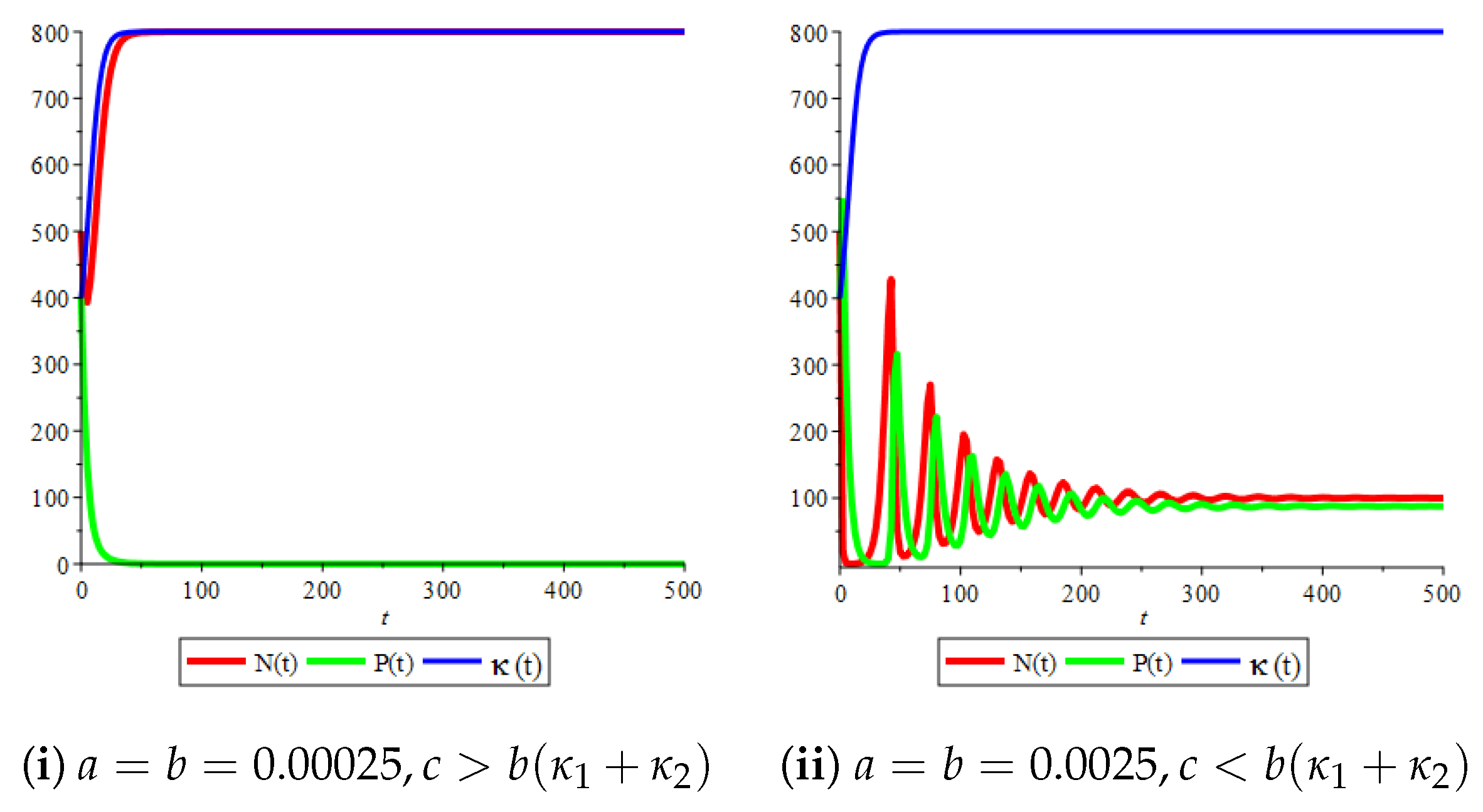
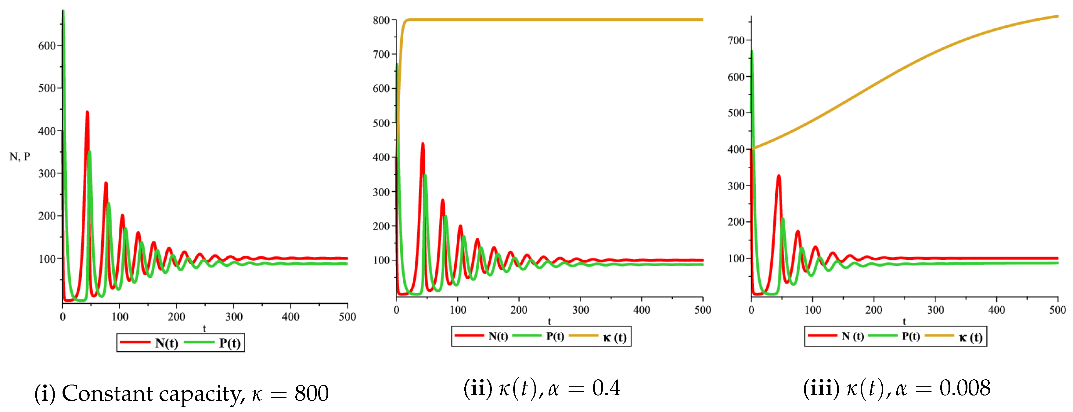
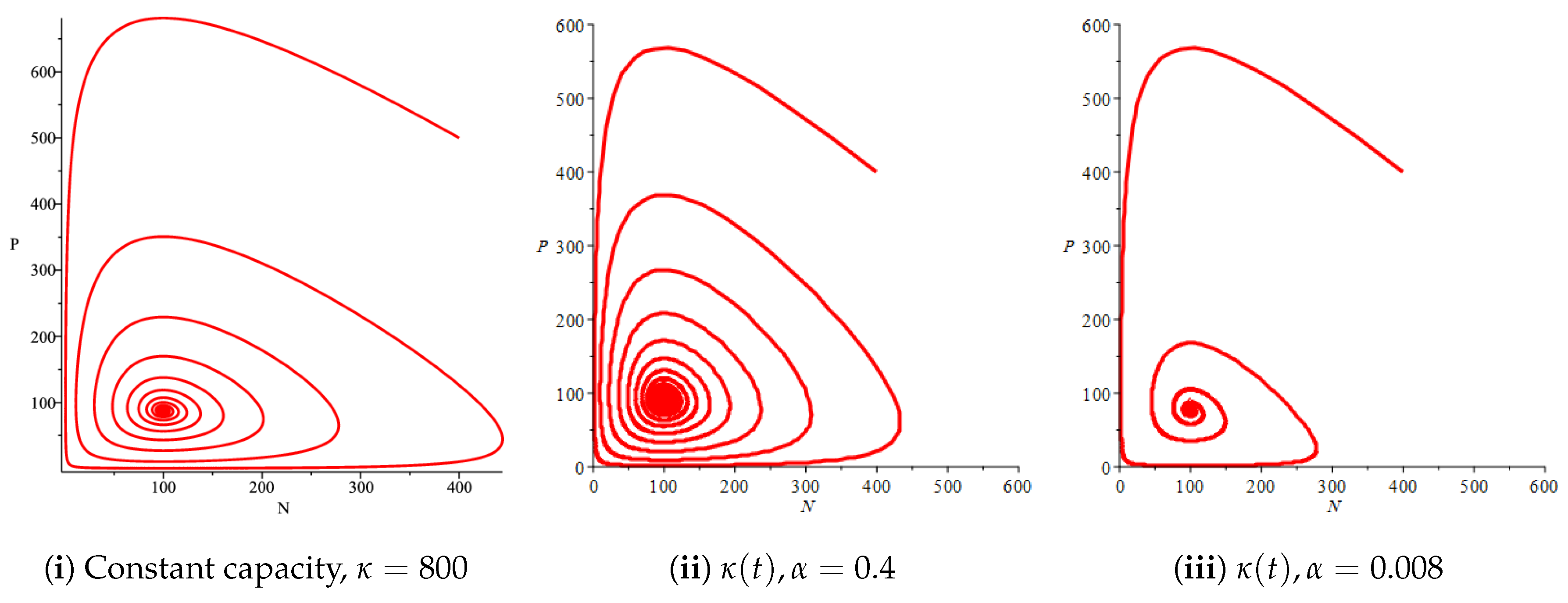
Figure 1(i) illustrates the case when the prey and the predator reach the stable equilibrium point ; that is, the prey follows the curve of carrying capacity, whereas the predator is extinct if . Figure 1(ii) demonstrates the case where the prey and the predator reach the stable equilibrium point with . The prey and predator populations exhibit damped oscillations before reaching the asymptotically stable spiral equilibrium point. These dynamics are similar to the constant carrying capacity case. However, if the growth rate of variable carrying capacity is very small, then the periodicity in the solutions of the systems decrease its magnitude. Additionally, the solutions reach the stable equilibrium faster compared to the constant carrying capacity case and compared to the variable carrying capacity case with a higher growth rate, as illustrated in Figure 2. In addition, Figure 3 illustrates the effect of variable carrying capacity on the phase space of the model, which confirms that less time is needed for the prey and predator populations to reach their equilibrium values when the growth rate of carrying capacity is very small, which can be seen from the trajectories in the neighbourhood of the asymptotically stable spiral point.
3. Prey–Predator Model with Holling Type II Functional Response
A predator has to devote a certain time to search, catch, and consume its prey. If the prey density increases then searching becomes easier, but consuming prey takes the same amount of time. The functional response is therefore an increasing function of the prey density, obviously equal to zero at zero prey density, approaching a finite time at high densities. If the predator hunts different types of prey, then the functional response should increase as a power greater than 1 (usually 2). According to functional response, it can be expressed that there should exist a saturation effect; that is, the predator’s birth rate should tend toward a finite limit at high prey densities.
Here, in this section, we consider the prey–predator model with Holling type II functional response with variable carrying capacity.
3.1. Model Building
The prey–predator model with Holling type II functional response with logistic carrying capacity is governed by the following system of equations:
where is the handling parameter.
3.2. Mathematical Analysis of the Model
System (3) has six equilibrium points; namely: , ,, , , , . Note that and exist iff and , respectively.
As noted before, the carrying capacity is independent of the other two variables, so the equilibrium points , and are unstable; the local stability of the remaining equilibrium points is illustrated in the following theorem.
Theorem 3.
The local stability of the equilibrium points , and of System (3) is given by the following.
- (i)
- is unstable.
- (ii)
- is locally asymptotically stable if .
- (iii)
- is locally asymptotically stable if .
Proof.
The Jacobian matrix of the system is given by
By evaluating the Jacobian matrix at each equilibrium point, we have the following.
Clearly, is one of the eigenvalues. The other two eigenvalues are the eigenvalues of the reduced matrix:
where its characteristic polynomial is
Using Routh–Hurwitz Criteria, in order for this point to be locally stable, we should have:
and . ☐
The global stability for the equilibrium point is stated in the following theorem.
Theorem 4.
The equilibrium point is globally stable if in the positive quadrant of the plane.
Proof.
The proof is similar to the proof of Theorem 2. ☐
Note that, although is globally stable in the 2D phase plane, it can still be unstable in the 3D phase space of the full System (3)
The following theorem states the possibility of occurrence of Hopf bifurcation.
Theorem 5.
System (3) undergoes a Hopf bifurcation at the positive equilibrium when .
Proof.
The eigenvalues of the linearized system around the equilibrium point are and
where
Now, at ,
and
Therefore, from Hopf Theorem [12], the proof is concluded.
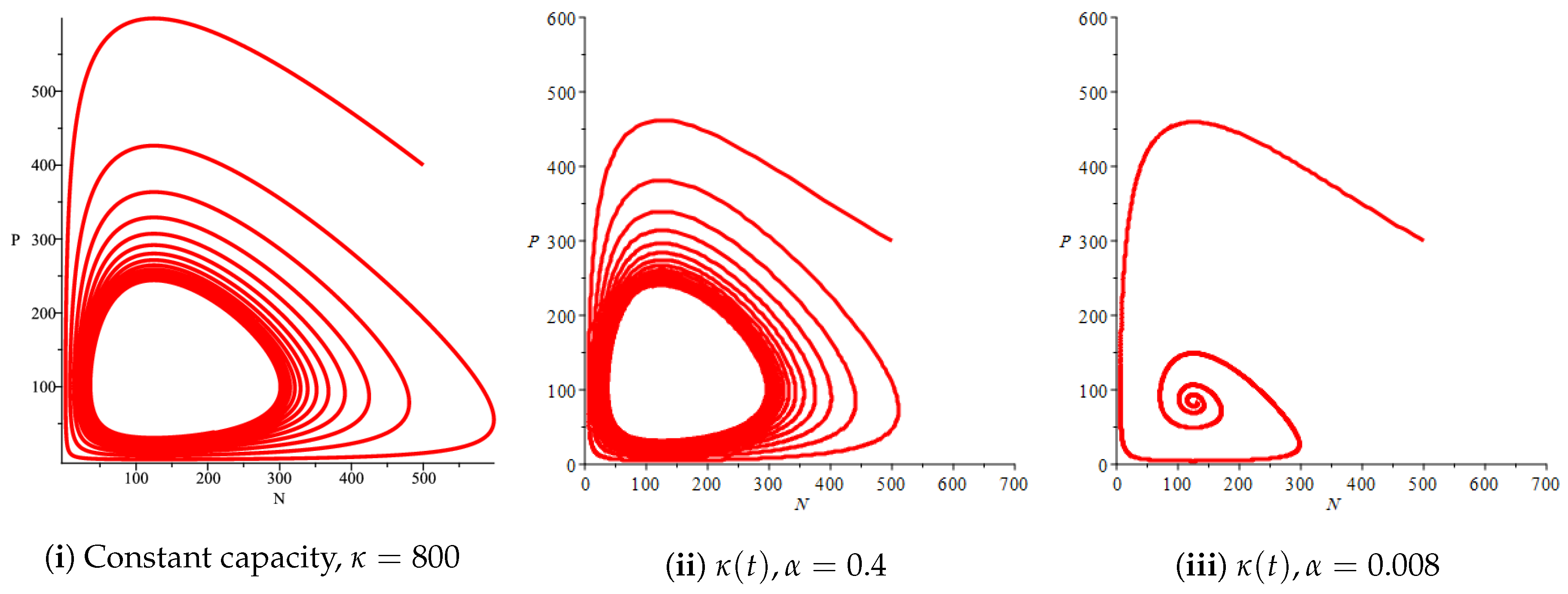
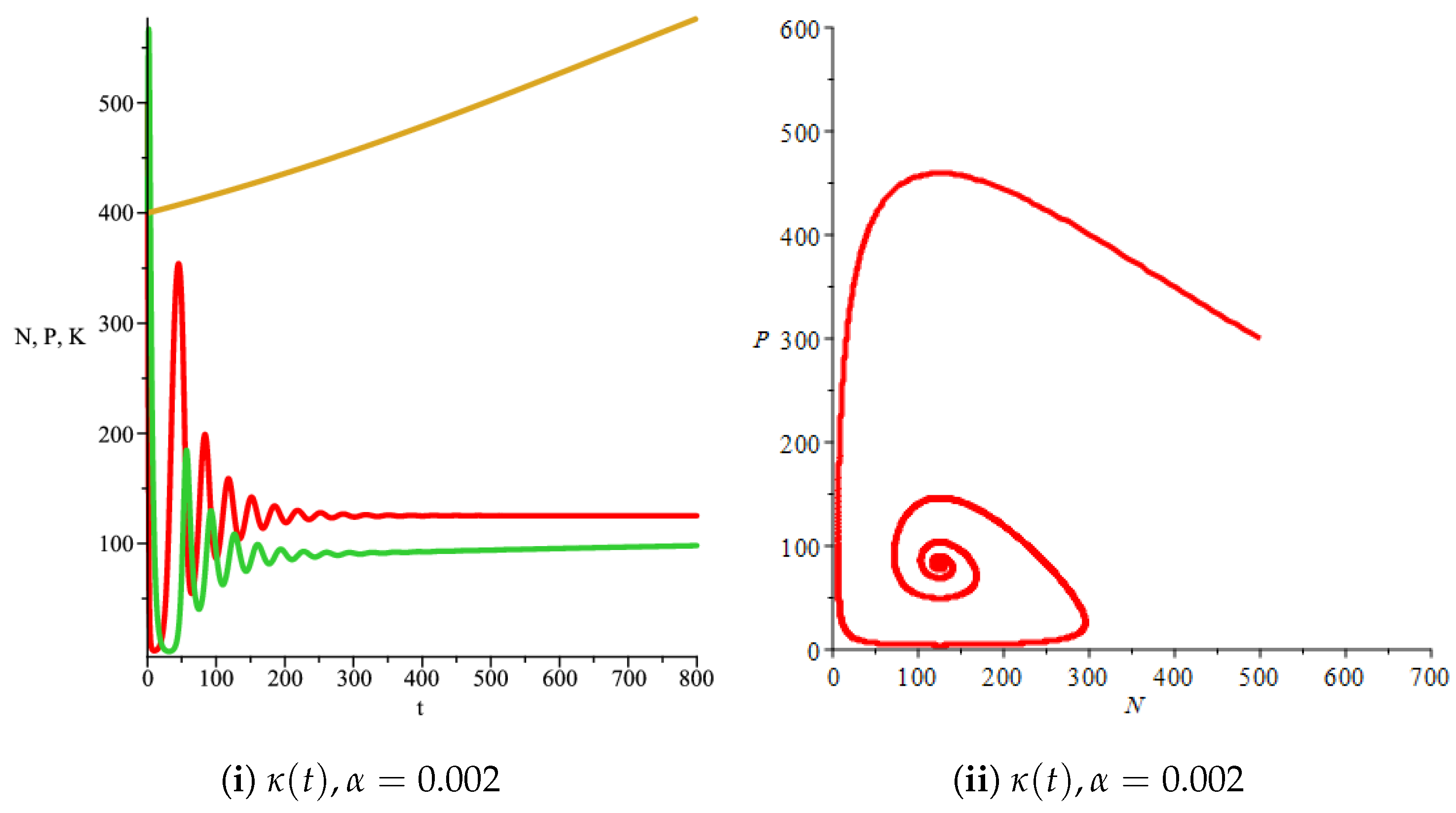
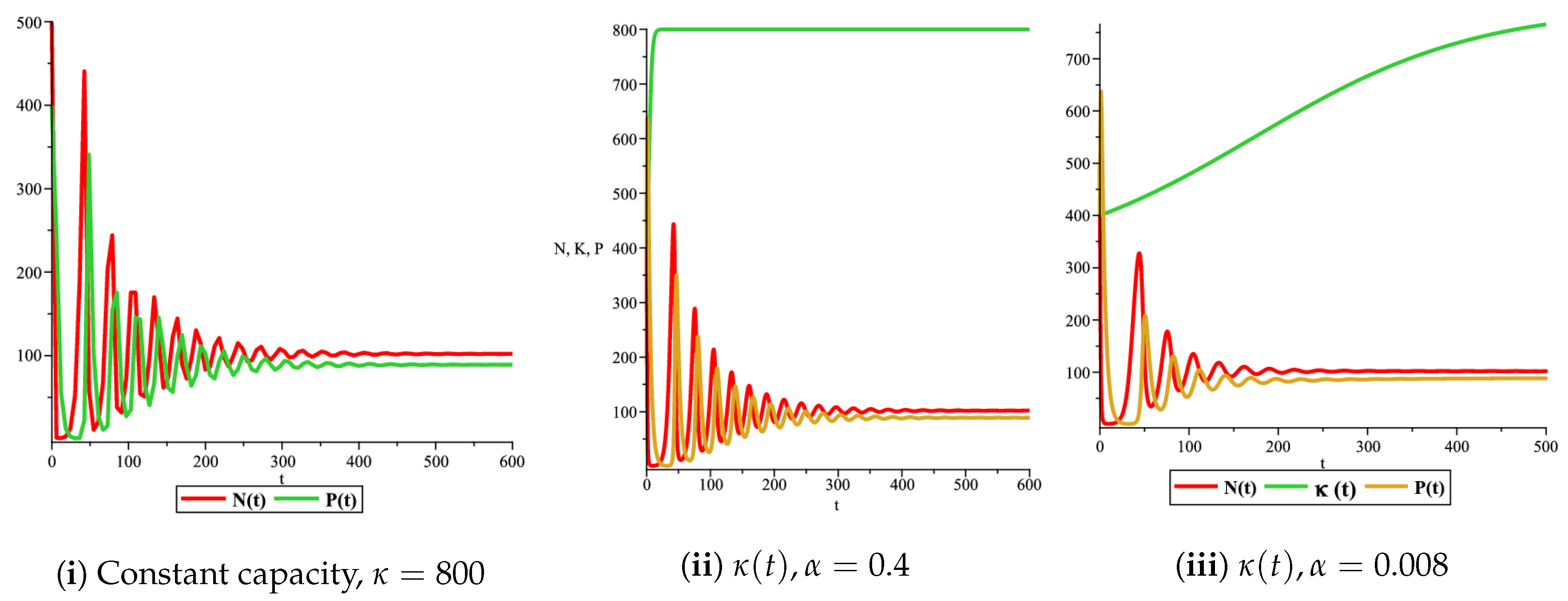
3.3. Numerical Simulation and Discussion
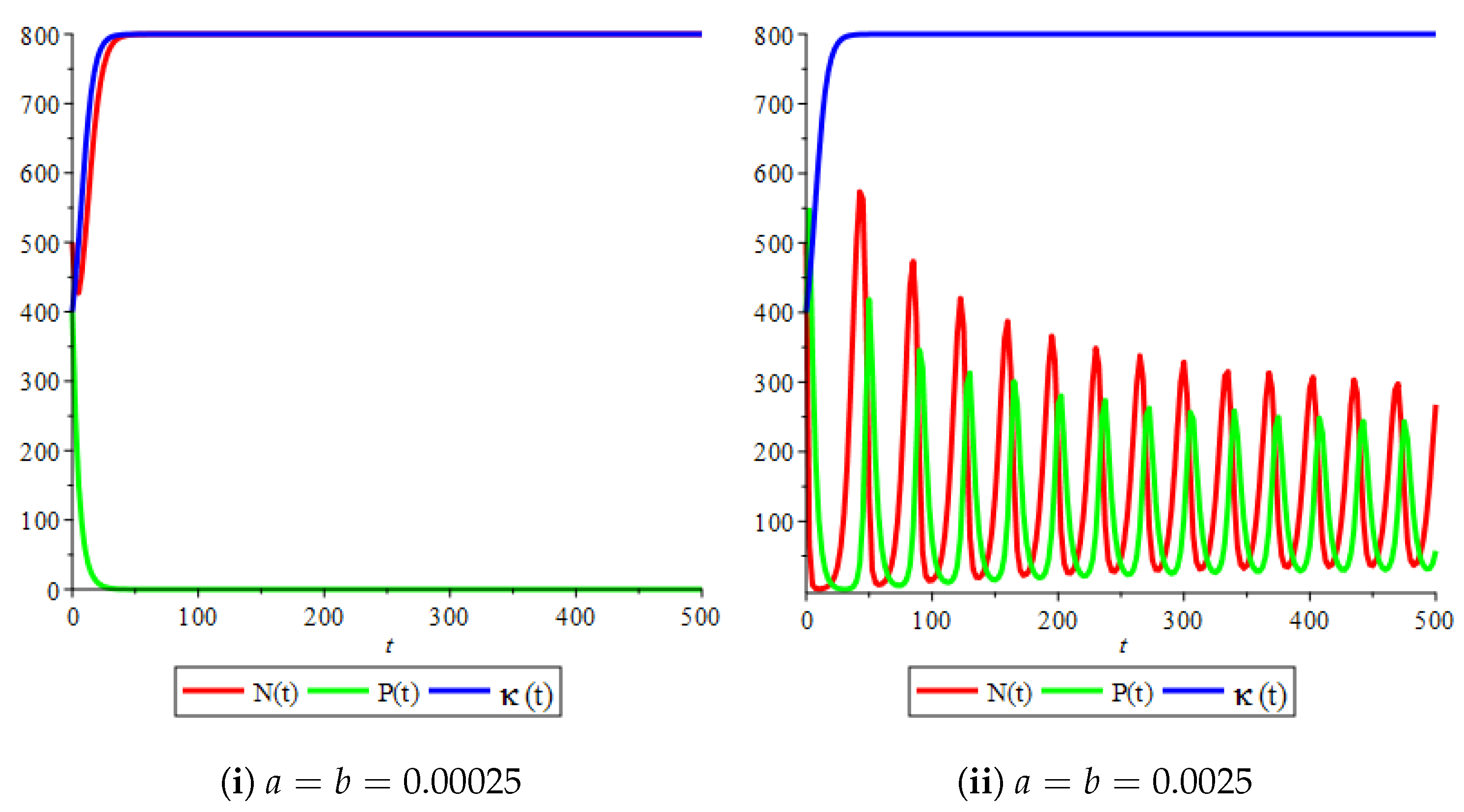
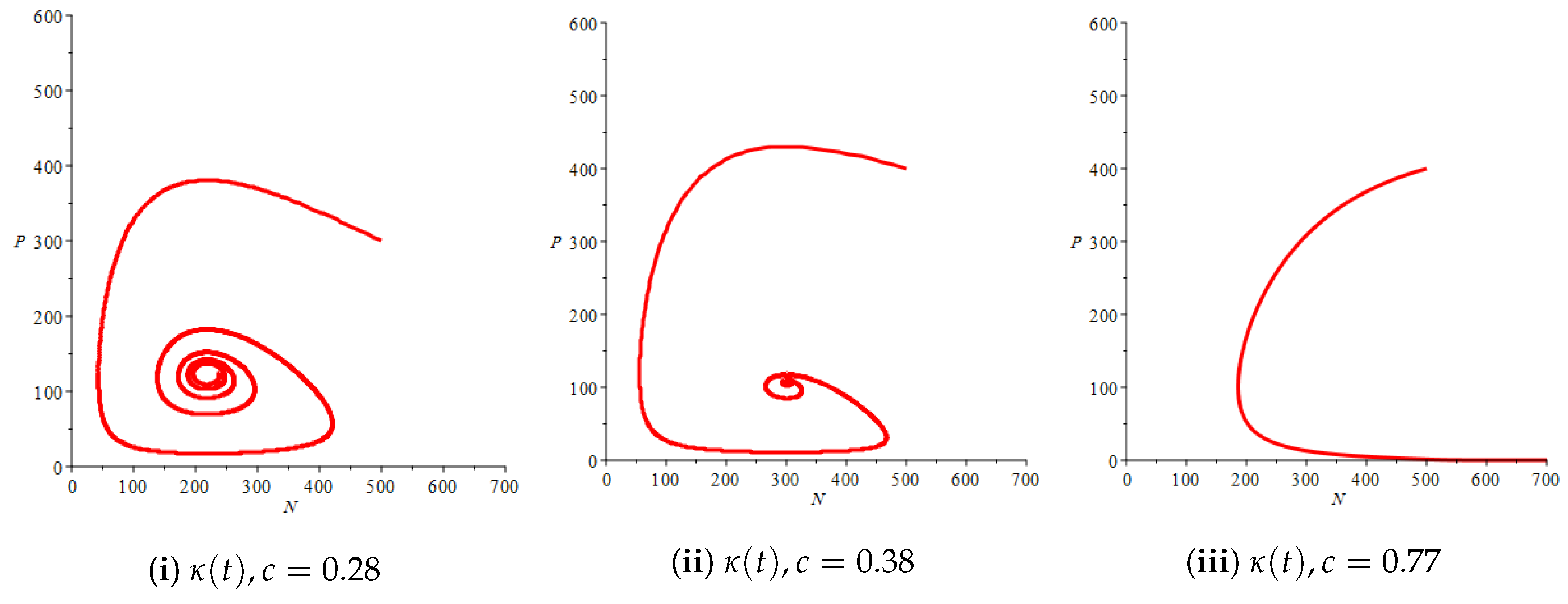
Figure 4(i) illustrates the case where the prey and the predator reach the stable equilibrium point ; that is, the prey follows the curve of carrying capacity, whereas the predator is extinct if . While Figure 4(ii) demonstrates the stability of if with , and . We can see from Figure 4 that the predator and prey populations exhibit damped oscillations. Moreover, these oscillations decrease in magnitude for smaller values of the carrying capacity growth rate as illustrated in Figure 5. This effect can also be seen in Figure 6, which demonstrates the phase space of the model where we have a stable limit cycle. However, when we reduce the growth rate to be much smaller, the effect of the variable carrying capacity is to convert the stable limit cycle into a spirally stable equilibrium point as shown in Figure 7. In addition, when we reduce the handling parameter , the prey and the predator populations exhibit damped oscillations before reaching an asymptotically stable spiral equilibrium point and the effect of variable carrying capacity is the same as in the Holling type I, that is, the periodicity in the solutions of the systems decrease its magnitude and reach to the stable equilibrium faster than the systems with constant carrying capacity as shown in Figure 8 and Figure 9. The effect of the death rate of the predator, which is the bifurcation parameter, on the prey and predator population dynamics is illustrated in Figure 10 and Figure 11. It can be seen that, when the death rate is small (up to around ) the populations are periodic and reach a stable limit cycle. If the death rate is higher (up to around ), the populations exhibit damped oscillations and reach the asymptotically stable spiral equilibrium point , which represents the co-existence of both populations. If the death rate is even higher than around , then the two populations reach the asymptotically stable point , which represents the extinction of the predator and the existence of only the prey.
4. Conclusions
Our aim in this paper is to examine the effect of variable carrying capacity on the prey–predator dynamics. For this purpose, two prey–predator models with logistic carrying capacity have been considered, namely, prey–predator models with Holling type I and type II functional responses. Stability analysis and numerical solutions of the two models were obtained, and the results were displayed graphically. Our results show that, when interaction between the prey and the predator populations was considered to be of Holling type I functional response, the prey and predator populations exhibit damped oscillations before reaching the asymptotically stable spiral equilibrium point. However, if the growth rate of the variable carrying capacity is very small, then the oscillations decrease in magnitude. The solutions were also found to reach the stable equilibrium faster compared to the constant carrying capacity case and compared to the variable carrying capacity case with higher growth rate. In addition, the equilibrium point representing existence of prey and the extinction of the predator with maximum carrying capacity was found to be globally asymptotically stable under a certain condition in the plane; however, it might not be stable in the 3D plane.
In the case when the interaction between the prey and the predator was considered to follow Holling type II functional response, our results showed that, when a limit cycle exists and when the growth rate of the logistic variable carrying capacity is very small, the stable limit cycle converted into a spirally stable equilibrium point. Our results also showed that this system undergoes a Hopf bifurcation at the positive equilibrium representing the co-existence of prey and predator with the maximum carrying capacity under a certain value of death rate. The equilibrium point representing the existence of prey and the extinction of predator with the maximum carrying capacity was found to be globally asymptotically stable under a certain condition in the plane. It is worth nothing that this might not be the case in the 3D plane.
Moreover, when the handling parameter was reduced, the prey and the predator were found to exhibit damped oscillations and then reached an asymptotically stable spiral equilibrium point. The effect of variable carrying capacity in this case is the same as in in Holling type I; that is, the periodicity in the solutions of the system decreases in magnitude and reaches the stable equilibrium faster than the system with constant carrying capacity. Finally, when the death rate of predators, which was taken to be the bifurcation parameter, was increased, the prey and the predator dynamics changed from having periodic behaviour that, by exhibiting damped oscillations and reaching an asymptotically stable spiral equilibrium point representing the co-existence of both populations, reached a stable limit cycle for small values of the death rate of the predator to a situation where the two populations reach an asymptotically stable point representing the existence of the prey population only in the case of the higher predator’s death rate.
Author Contributions
I.M.E. and N.S.A.-S. proposed and formulated the models; M.K.A.A.-M. carried out the mathematical analysis and the numerical simulations; M.K.A.A.-M., N.S.A.-S., and I.M.E. wrote the paper.
Acknowledgments
M.K.A.A.-M. acknowledges with thanks the support from the Ministry of Education, Sultanate of Oman. The authors would like to acknowledge the support form Sultan Qaboos University. The authors would also like to thank two anonymous reviewers whose comments improved the quality and readability of the paper.
Conflicts of Interest
The authors declare that there is no conflict of interest.
References
- Green, J.L.; Hastings, A.; Arzberger, P.; Ayala, F.J.; Cottingham, K.L.; Cuddington, K.; Davis, F.; Dunne, J.A.; Fortin, M.; Gerber, L.; et al. Complexity in Ecology and Conservation: Mathematical, Statistical, and Computational Challenges. BioScience 2005, 55, 501–510. [Google Scholar] [CrossRef]
- Krebs, C.J. Ecology the Experimental Analysis of Distribution and Abundance; Pearson Education, Inc.: Upper Saddle River, NJ, USA, 2009. [Google Scholar]
- Monte-Luna, D.; Brook, B.W.; Zetina-Rejón, M.J.; Cruz-Escalona, V.H. The carrying capacity of ecosystems. Glob. Ecol. Biogeogr. 2004, 13, 485–495. [Google Scholar] [CrossRef] [Green Version]
- Cohen, J.E. How many people can the earth support? Sciences 1995, 35, 18–23. [Google Scholar] [CrossRef]
- Waggoner, P.E. How much land can ten billion people spare for nature? Daedalus 1995, 125, 73–93. [Google Scholar]
- Meerschaert, M.M. Mathematical Modelling; Academic Press: Waltham, MA, USA, 2013. [Google Scholar]
- Ludwig, D.; Hilborn, R.; Walters, C. Uncertainty, resource exploitation, and conservation: Lessons from history. Science 1993, 260, 17. [Google Scholar] [CrossRef] [PubMed]
- Meyer, P. Bi logistic growth. Technol. Forecast. Soc. Chang. 1994, 47, 82–102. [Google Scholar] [CrossRef]
- Shepherd, J.J.; Stojikov, L. The logistic population model with slowly varying carrying capacity. Anziam J. 2007, 47, 492–506. [Google Scholar] [CrossRef]
- Allen, L.S. An Introduction to Mathematical Biology; Pearson Education, Inc.: Upper Saddle River, NJ, USA, 2007. [Google Scholar]
- Strogatz, S.H. Nonlinear Dynamics and Chaos: With Application to Physics, Biology, Chemistry and, Engineering; Perseus Books Publishing: Philadelphia, PA, USA, 2014. [Google Scholar]
- Kuznesov, Y.A. Elements of Applied Bifurcation Theorem; Springer: New York, NY, USA, 1998. [Google Scholar]
Figure 1.
Prey–predator model with Holling type I functional response and logistic carrying capacity, stability of and for
Figure 1.
Prey–predator model with Holling type I functional response and logistic carrying capacity, stability of and for

Figure 2.
Effect of the logistic variable capacity on the prey–predator model with linear response for
Figure 2.
Effect of the logistic variable capacity on the prey–predator model with linear response for

Figure 3.
Effect of the logistic variable varying capacity on the phase space of the prey and predator model with linear response for
Figure 3.
Effect of the logistic variable varying capacity on the phase space of the prey and predator model with linear response for

Figure 4.
Prey–predator model with Holling type II functional response and logistic carrying capacity, stability of and ,
Figure 4.
Prey–predator model with Holling type II functional response and logistic carrying capacity, stability of and ,

Figure 5.
Effect of logistic carrying capacity on prey–predator model with Holling type II functional response for
Figure 5.
Effect of logistic carrying capacity on prey–predator model with Holling type II functional response for
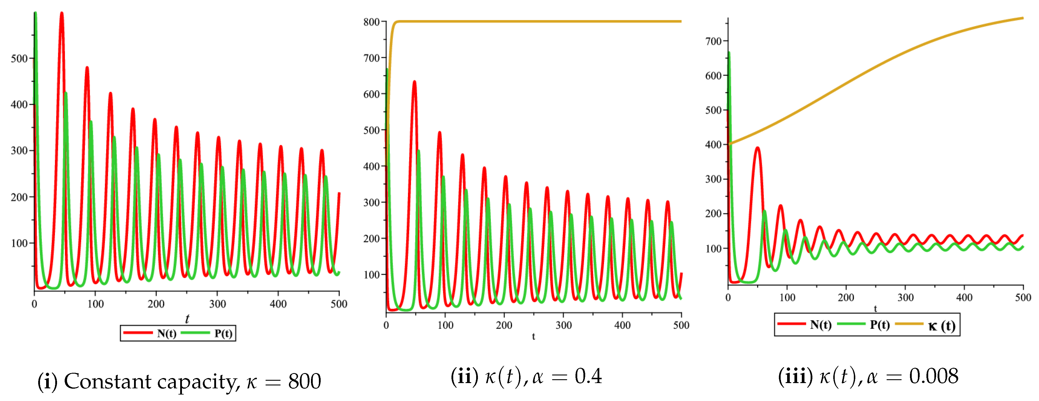
Figure 6.
Effect of the logistic variable carrying capacity on the phase space of the prey–predator model with Holling type II functional response for
Figure 6.
Effect of the logistic variable carrying capacity on the phase space of the prey–predator model with Holling type II functional response for

Figure 7.
Effect of logistic carrying capacity on prey–predator model with Holling type II functional response,
Figure 7.
Effect of logistic carrying capacity on prey–predator model with Holling type II functional response,

Figure 8.
Effect of logistic carrying capacity on prey–predator model with Holling type II functional response,
Figure 8.
Effect of logistic carrying capacity on prey–predator model with Holling type II functional response,

Figure 9.
Effect of the logistic variable carrying capacity on the phase space of the prey and predator model with Holling type II functional response for
Figure 9.
Effect of the logistic variable carrying capacity on the phase space of the prey and predator model with Holling type II functional response for
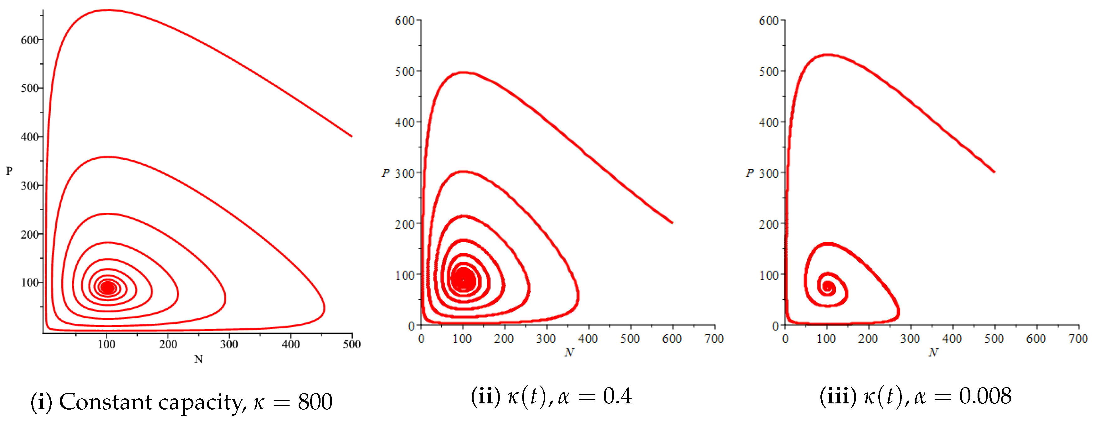
Figure 10.
Effect of the bifurcation parameter on the prey–predator model with Holling type II functional response,
Figure 10.
Effect of the bifurcation parameter on the prey–predator model with Holling type II functional response,
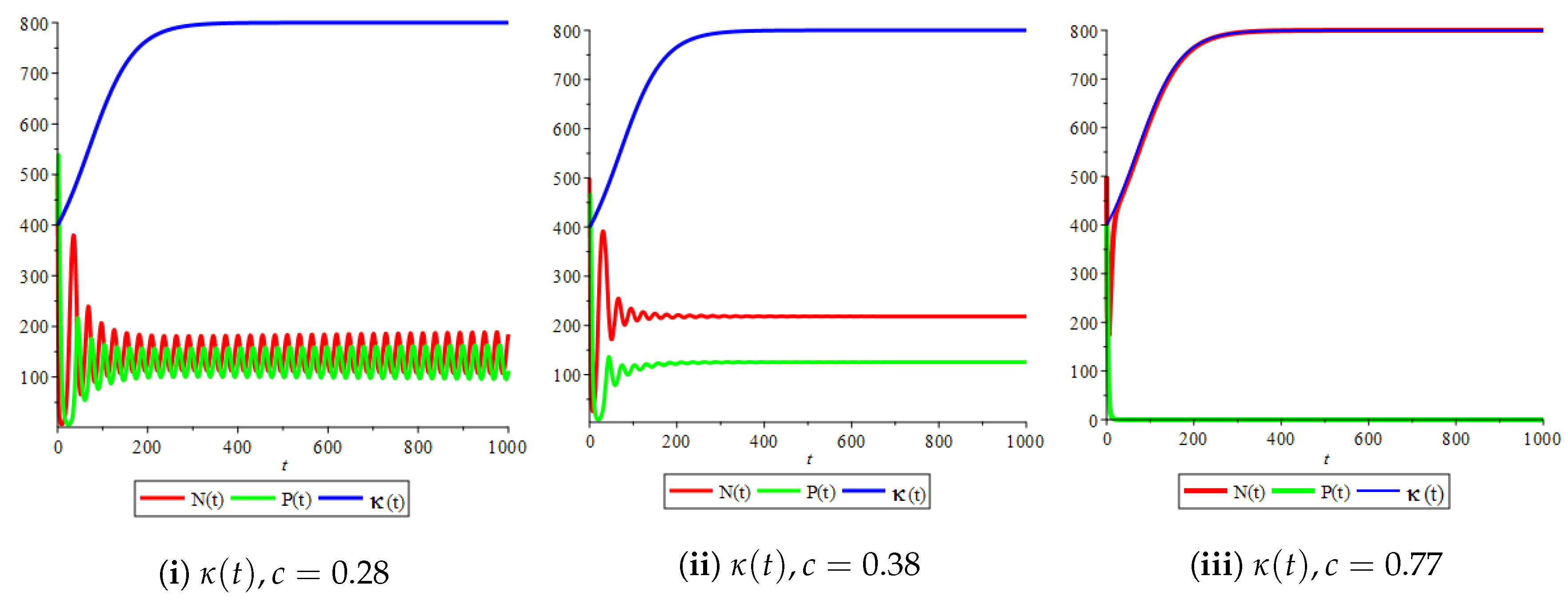
Figure 11.
Effect of the bifurcation parameter on the phase space of the prey–predator model with Holling type II functional response with
Figure 11.
Effect of the bifurcation parameter on the phase space of the prey–predator model with Holling type II functional response with

© 2018 by the authors. Licensee MDPI, Basel, Switzerland. This article is an open access article distributed under the terms and conditions of the Creative Commons Attribution (CC BY) license (http://creativecommons.org/licenses/by/4.0/).
Share and Cite
MDPI and ACS Style
Al-Moqbali, M.K.A.; Al-Salti, N.S.; Elmojtaba, I.M. Prey–Predator Models with Variable Carrying Capacity. Mathematics 2018, 6, 102. https://doi.org/10.3390/math6060102
AMA Style
Al-Moqbali MKA, Al-Salti NS, Elmojtaba IM. Prey–Predator Models with Variable Carrying Capacity. Mathematics. 2018; 6(6):102. https://doi.org/10.3390/math6060102
Chicago/Turabian StyleAl-Moqbali, Mariam K. A., Nasser S. Al-Salti, and Ibrahim M. Elmojtaba. 2018. "Prey–Predator Models with Variable Carrying Capacity" Mathematics 6, no. 6: 102. https://doi.org/10.3390/math6060102
Note that from the first issue of 2016, this journal uses article numbers instead of page numbers. See further details here.