Decomposition of Dynamical Signals into Jumps, Oscillatory Patterns, and Possible Outliers

1
National Physical Laboratory, Teddington, Middlesex TW11 0LW, UK
2
Department of Computer Science, College of Science, University of Baghdad, Aljadirya, Baghdad 10071, Iraq
*
Author to whom correspondence should be addressed.
Mathematics 2018, 6(7), 124; https://doi.org/10.3390/math6070124
Submission received: 31 January 2018
/
Revised: 30 May 2018
/
Accepted: 19 June 2018
/
Published: 16 July 2018
(This article belongs to the Special Issue Chaos and Randomness of Discrete Dynamical Systems: Their Use in Applied Science)
Abstract
:In this note, we present a component-wise algorithm combining several recent ideas from signal processing for simultaneous piecewise constants trend, seasonality, outliers, and noise decomposition of dynamical time series. Our approach is entirely based on convex optimisation, and our decomposition is guaranteed to be a global optimiser. We demonstrate the efficiency of the approach via simulations results and real data analysis.
1. Introduction
1.1. Motivations
The goal of the present work is to propose a simple and efficient scheme for time series decomposition into trend, seasonality, outliers, and noise components. As is well known, estimating the trend and the periodic components play a very important role in time series analysis [1,2,3]. Important applications include financial time series [4,5], epidemiology [6], climatology [7], control engineering [8], management [9], and airline data analysis [10].
The trend and seasonality decomposition is often dealt with in a suboptimal sequential scheme and rarely in a joint procedure. Estimating the trend and the seasonality components can be addressed via many different techniques relying on filtering and/or optimisation of various criteria. It might not be always clear what global optimisation problem is actually solved by the successive methods employed. Moreover, we are not aware of any method that incorporates outlier detection into the procedure.
In this short note, we present a joint estimation technique based on recent approaches based on convex optimisation, namely -trend Filtering [11] and nuclear norm penalised low rank approximation of Hankel matrices, combined with an outlier detection scheme. Low rank estimation and outlier detection is performed using robust principal component analysis (PCA) [12]. Projection onto Hankel matrices is straightforward using averaging along diagonals. The whole scheme aims at providing a flexible and efficient method for time series decomposition based on convex analysis and fast algorithms, and as such aligns with the philosophy of current research in signal processing and machine learning [13].
Let us now introduce some notations. The time series we will be working with, denoted by is assumed to be decomposable into four components
where denotes the trend, denotes a signal that can be decomposed into a sum of few complex exponential sums, is a sparse signal representing rare outliers, and denotes the noise term.
1.2. Previous Works
More than often, the components of time series are estimated in a sequential manner.
1.2.1. Piecewise Constant Trend Estimation
A nice survey on trend estimation is [14]. Traditional methods include model based approaches using, e.g., state space models [15] or nonparametric approaches such as the Henderson, LOESS [16], and Hodrick–Prescott filters [17]. Some comparisons can be found in [4]. More recent approaches include empirical mode decomposition [14] and wavelet decompositions [18]. A very interesting approach called -trend filtering was recently proposed by [11] among others. This method allows for retrieval of piecewise constants or, more generally, piecewise polynomial trends from signals using -penalised least squares. In particular, this type of analysis is the perfect tool for segmenting time series and detecting model changes in the dynamics. These methods have been recently approach by statistical tools in [19,20,21,22].
1.2.2. Seasonality Estimation
Seasonality can also be addressed using various approaches [23,24]. Unit root tests sometimes allow for detection of some seasonal components. Periodic autoregressive models have been proposed as a simple and efficient model with many applications in, e.g., business [25], medicine [26], and hydrology [27]. The relationship between seasonality and cycle can be hard to formalise when dependencies are present [24]. Another line of research is based on Prony’s method [28,29]. Prony’s method is based on the fact that any signal which is the sum of exponential functions can be put into a Hankel matrix, whose rank will be the number of exponential components. Applications are multiple in signal processing [30], electromagnetics [31], antennas [32], medicine [33], etc., although they are not robust to noise. This approach can be enhanced using alternating projections such as in [34]. There are now many works on improving Prony’s method. For our purposes, we will concentrate on a rank regularised Prony-type approach. The rank regularisation will be performed by using a surrogate such as the nuclear norm for matrices.
1.2.3. Joint Estimation
Seasonality and trend estimation can be performed using, e.g., general linear abstraction of seasonality (GLAS), widely used in econometrics [4]. Existing software, e.g., X-12-ARIMA, TRAMO-SEATS, and STAMP, is available for general purpose time series decomposition, but such programs do not provide the same kind of analysis as the decomposition we provide in the present paper. For instance, it is well known that ARMA estimation is based on a non-convex likelihood optimisation step for which no current method can be proved to provide a global optimiser.
Singular spectrum analysis (SSA) is also widely used, and the steps of this algorithm are similar to those of PCA, but especially tailored for time series [14]. Neither a parametric model nor stationarity are postulated for the method to work. SSA seeks to decompose the original series into a sum of a small number of interpretable components such as trend, oscillatory components, and noise. It is based on the singular value decomposition of a specific matrix built from the time series. This makes SSA a model-free method and hence enables SSA to have a very wide range of applicability [35].
1.3. Our Contribution
The methodology developed in this work brings together several important discoveries from the last 10 years based on sparse estimation, in particular, non-smooth convex surrogates for cardinality and rank-type penalisations. As a result, we obtain a decomposition that is easily interpretable and that detects the location of possible abrupt model changes and of outliers. These features are not supplied by, e.g., the SSA approach, albeit of fundamental importance for quality assessment.
2. Background on Penalised Filtering, Robust PCA, and Componentwise Optimisation
We start with a short introduction to sparsity promoting penalisation in statistics, based on the main properties of one of the simplests avatars of this approach: the least absolute selection and shrinkage operator (LASSO) [19].
2.1. The Nonsmooth Approach to Sparsity Promoting Penalised Estimation: Lessons from the LASSO
All of the techniques that are going to be used in the paper resort to sparse estimation for vectors and spectrally sparse estimation for matrices. Sparse estimation has been a topic of extensive research in the last 15 years [36]. Our signal decomposition problem strongly relies on sparse estimation because jumps have sparse derivative [20], piecewise affine signals have sparse second order derivative [11], seasonal components can be estimated using spectrally sparse Hankel matrices (Prony’s method and its robustified version [37]), and outliers are sparse matrices [12].
Sparse estimation, the estimation of a sparse vector, matrix, or spectrally sparse matrix with possibly additional structure, usually consists in least squares minimisation under a sparsity constraint. Unfortunately, sparsity constraints are often computationally hard to deal with and, as surveyed in [36], one has to resort to convex relaxations.
Efficient convex relaxations for sparse estimation originally appeared in statistics in the context of regression [38]. The main idea is that the number of non-zero components of a vector can be convexified using the Fenchel bi-dual over the unit-ball. The resulting functional is nothing but the -norm of the vector. Incorporating an -norm penalty into the least-squares scheme is a procedure known as the LASSO in the statistics literature [39,40,41] and for joint variance and regression vector estimation [42]; see also [43] for very interesting modified LASSO-type procedures. Based on the same idea, spectral sparsity constraints can be relaxed using nuclear norm-type of penalisations in the matrix setting [36] and even in the tensor setting [44,45,46].
In the next paragraphs, we describe how these ideas apply to the different components of the signal.
2.2. Piecewise Constant Signals
When the observed signal is of the form
for , where is piecewise constant, with less than jumps, the corresponding estimation problem can be written as
where D is the operator which transforms a sequence into a sequence of successive differences.
This problem is unfortunately non-convex, and the standard approach to the estimation of is to replace the -norm with the norm of the vector of sucessive differences, which turns out to be known as the total variation penalised least-squares estimator defined as a solution to the following optimisation problem [20]:
Here, the penalisation term is a convexification of the function that counts the number of jumps in T. This estimation/filtering procedure suffers from the same hyper-parameter calibration as the LASSO. Many different procedures have been devised for this problem such as [47]. The method of [48] based on online learning can also be adapted to this context.
2.3. Prony’s Method
We will make great use of Prony’s method for our decomposition. We will indeed look for oscillating functions in the seasonal component. This can be expressed as the problem of finding a small sum of exponential functions. In mathematical terms, these functions are
where , are complex numbers.
Remark 1.
The adjoint operator consists of extracting a signal of size n from a Hankel matrix in the most canonical way, i.e. by extracting following the first column and then the last row in the most obvious way.
When the values have unit moduli, we obtain sigmoidal functions. Otherwise, a damping factor appears for certain frequencies, and one obtains a very flexible model for a general notion of seasonality.
Consider the sequence defined by (5). It is easy to notice that the matrix
is singular. Conversely, if belongs to the kernel of , then the sequence satisfies a difference equation of the type
The important fact to recall now is that the solutions to such difference equations form a complex vector space of dimension and all the exponential sequences are independent particular solutions that form a basis of this vector space.
Thus, and this is the cornerstone of Prony-like approaches to oscillating signals modelling, the highly nonlinear problem of finding the exponentials whose combinations reconstructs a given signal is equivalent to a simple problem in linear algebra. The main question now is whether this method is robust to noise. Unfortunately, the answer is no, and some enhancements are necessary in order to use this approach innoisy signals or time series analysis.
2.4. Finding a Low Rank Hankel Approximation
We will also need to approximate the Hankel matrix from the previous section by a low rank matrix. If no other constraint is imposed on this approximation problem, it turns out that this task can be efficiently achieved by singular value truncation. This is what is usually done in data analysis under the name of PCA.
From the applied statistics perspective, PCA, defined as a tool for high-dimensional data processing, analysis, compression, and visualisation, has wide applications in scientific and engineering fields. It assumes that the given high-dimensional data lie near a much lower-dimensional linear subspace. The goal of PCA is to efficiently and accurately estimate this low-dimensional subspace. This turns out to be equivalent to truncating the singular value decomposition (SVD), a fact also known as the Eckhart–Young Theorem, and this is exactly what we need for our low rank approximation problem. In mathematical terms, given a matrix , the goal is to simply find a low rank matrix , such that the discrepancy between and is minimised, leading to the following constrained optimisation
where is the target dimension of the subspace.
The problem we have to address here is the following generalisation: we have to approximate a Hankel matrix by a low rank Hankel matrix. These additional linear constraints seem innocent, but it nevertheless introduces an additional level of complexity. This problem can be efficiently addressed by solving the following decoupled problem
where is the target dimension of the subspace, and is a sufficiently large positive constant. Approximating this problem with a convex problem can be achieved by solving the following problem
3. Main Results
We now describe and analyse our method, which combines the total variation minimisation, the Hankel projection, and the SVD.
3.1. Putting It All Together
If one wants to perform the full decomposition and remove the outliers at the same time, we need to find a threefold decomposition of , where L is low rank and Hankel, O is a sparse signal-vector representing the outliers, and E is the error vector. This can be performed by solving the following optimisation problem.
Using the discussions of the former section based on using the norm as a surrogate to the non-convex functional, this problem can be efficiently relaxed into the following convex optimisation problem
where denotes the nuclear norm, i.e., the sum of the singular values.
This optimisation problem can be treated as a general convex optimisation problem and solved by any off-the-shelf interior point solver, after being reformulated as a semi-definite program. Many standard approaches are available for this problem. In the present paper, we choose an alternating projection method, which performs optimisation with respect to each variable one at a time.
3.2. A Component-Wise Optimisation Method
Our goal is to solve the following optimisation problem
Remark 2.
The optimisation step with respect to T is just the trend filtering optimisation problem applied to .
One way to approach this problem is to devise an Alternating Direction of Multipliers Method (ADMM) type of algorithm. For this purpose, let us define the Lagrange function
and let denote the constraint set
Let denote the augmented Lagrange function given by
The ADMM consists in putting the subspace alternating method to work, including an update of the Lagrange mutiplier G. It is described in Algorithm 1 below. A very nice presentation of this type of algorithm is given in [50].
| Algorithm 1: ADMM-based jump-seasonality-outlier decomposition |
 |
For the sake of practical relevance, we also include the following method consisting of successive optimisation steps and can be seen essentially as an acceleration of the ADMM approach. Each loop successively solves the PCA and the and total variation penalised least-squares optimisation problems, as well as the projection onto the space of Hankel matrices. It is described in Algorithm 2 below.
| Algorithm 2: Componentwise jump-seasonality-outlier decomposition |
 |
3.3. Convergence of the Algorithm
The convergence of the ADMM Algorithm 1 is guaranteed by the theory provided in [51]. Concerning Algorithm 1, one can check that it corresponds to taking in the Lagrange function . The convergence of the method is then straightforward. As is set to to grow to , the respective solutions provided by the two algorithms will become correspondingly closer to each other, up to any pre-specified accuracy.
3.4. Numerical Experiments
In this section, we present some preliminary experiments which illustrate the behavior of the method on simulated data and real data. The method we implemented uses additional debiasing, and Frobenius projection instead of projection for better scalability.
3.4.1. Simulated Data
In this section, we provide some illustrations of the algorithm on simulated data. Signals are generated with various seasonal patterns, piece-wise constant components and outliers. In all cases, we assume that the data is subject to Gaussian noise with an associated standard deviation of 2 units.
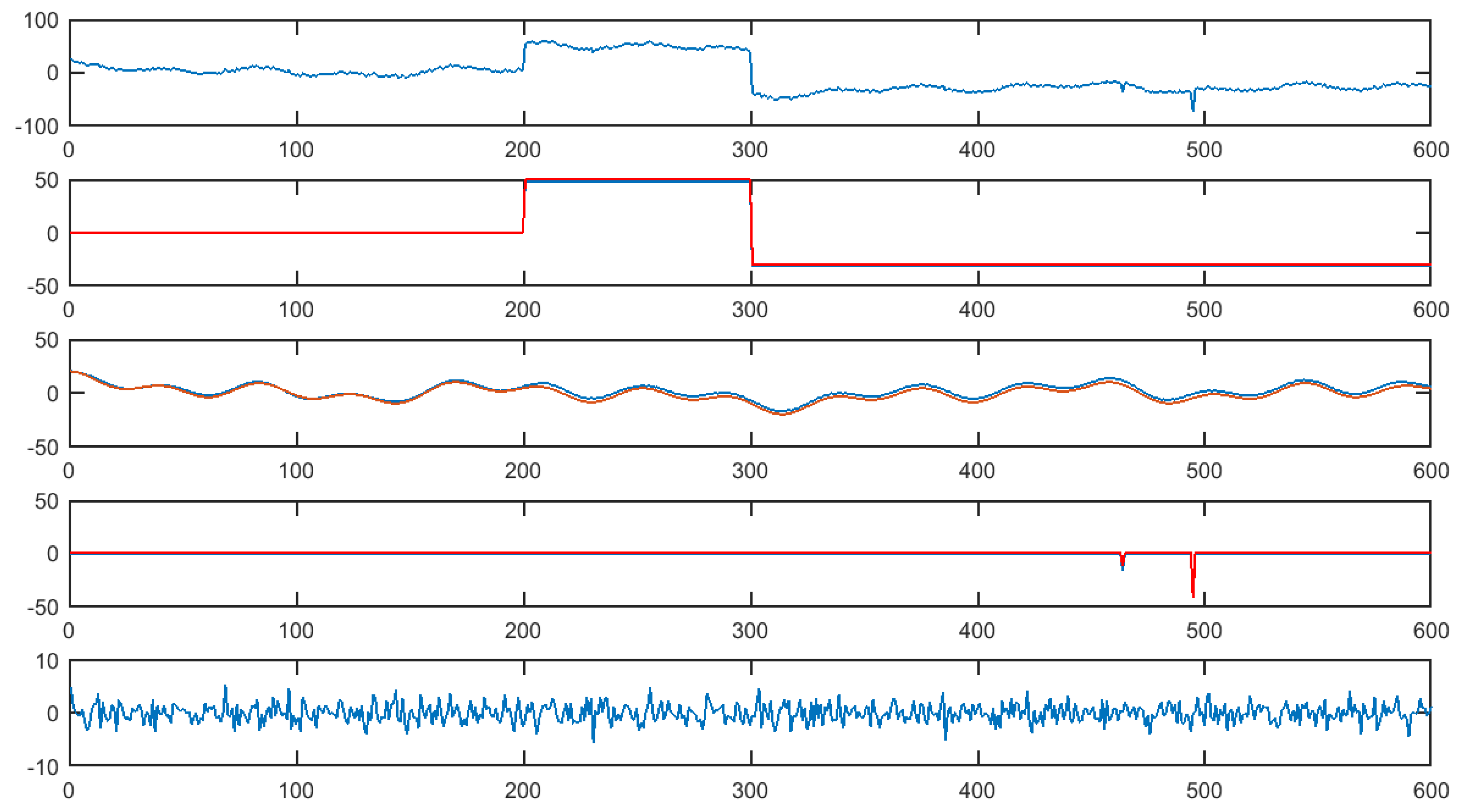
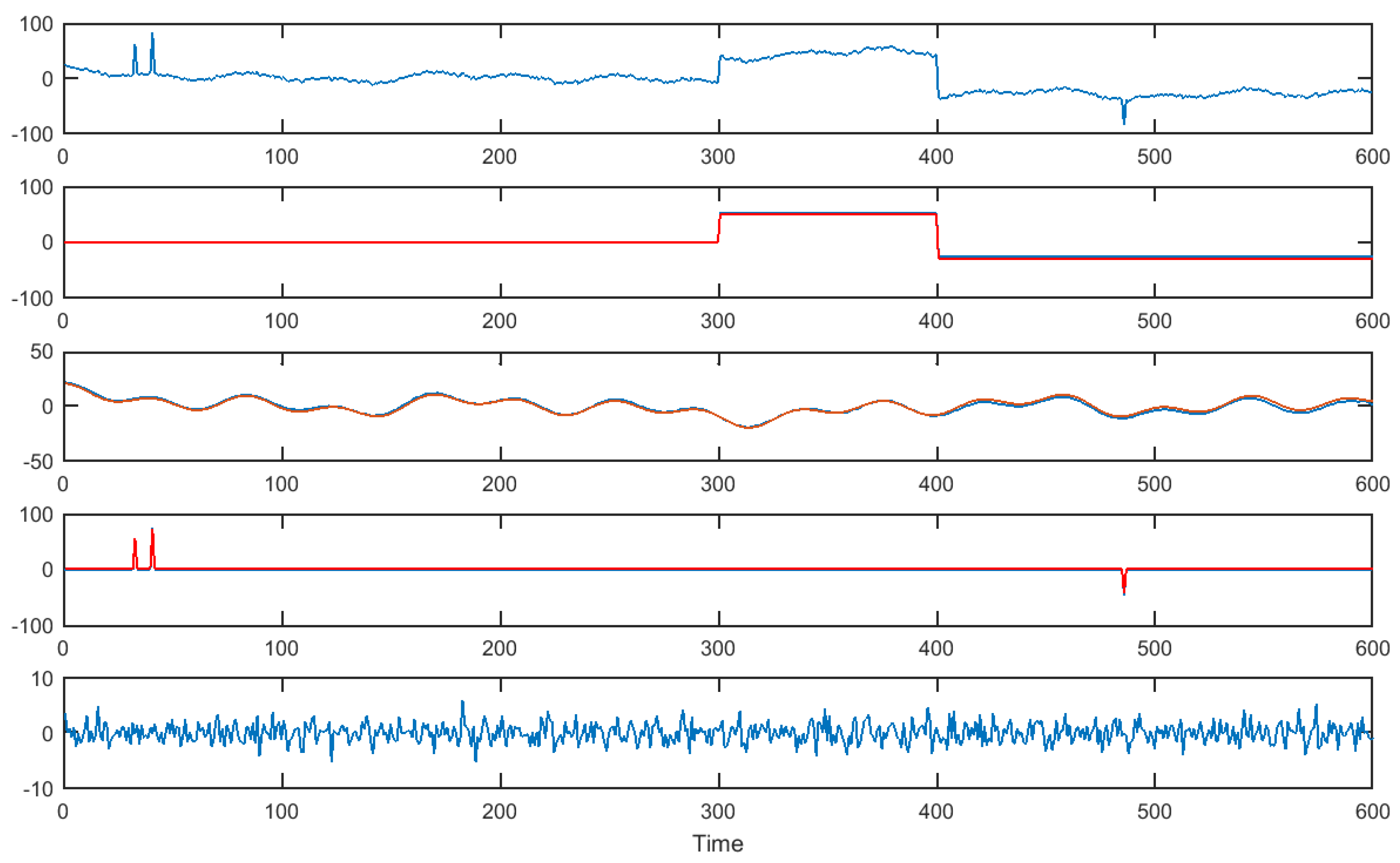
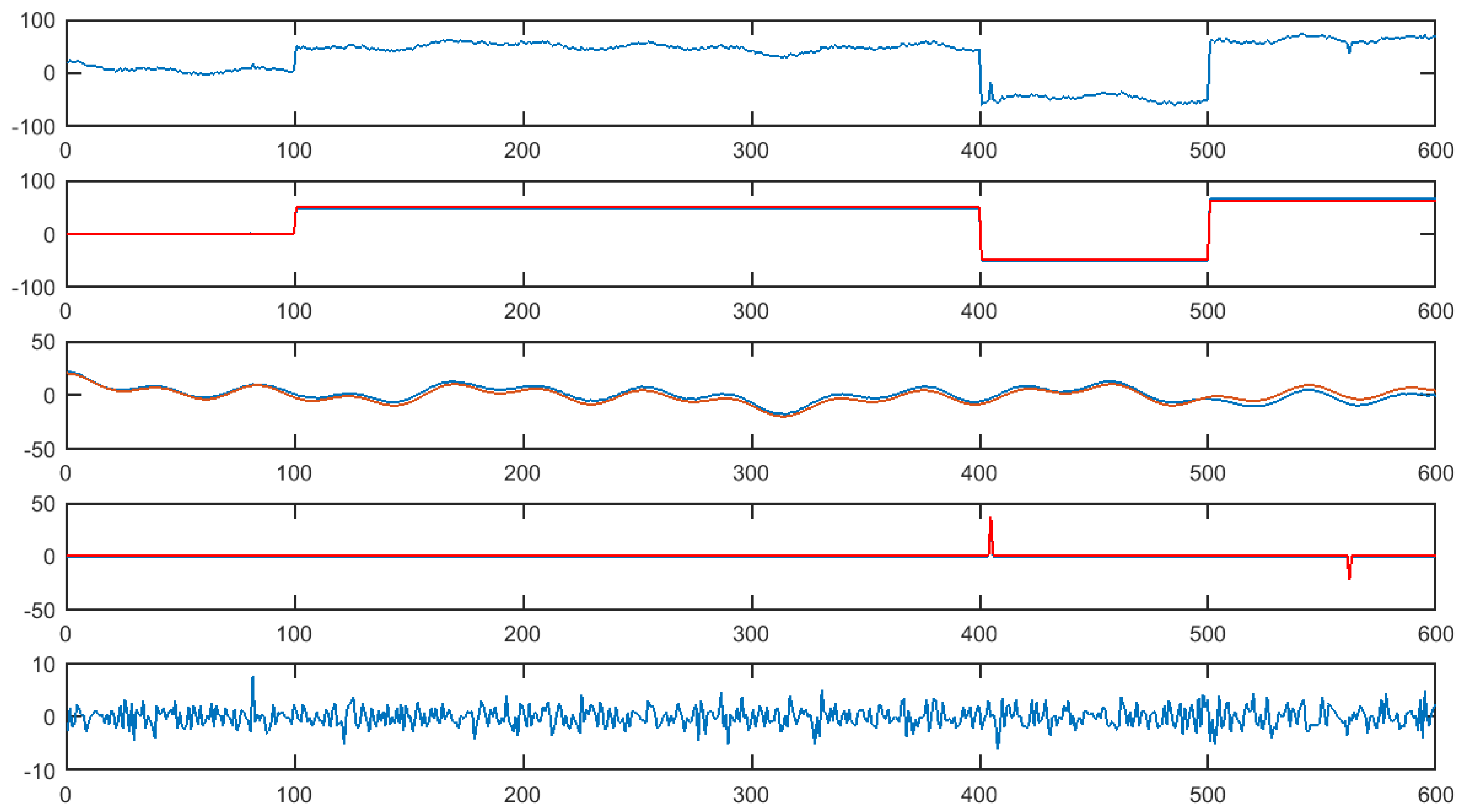
Figure 1, Figure 2 and Figure 3 demonstrate the decomposition of a signal with 2, 3, and 5 outliers, respectively. The top block of each figure is the signal itself. The second block is the extracted piecewise constant component. The red line is the true signal, and the blue one is the estimate. The third block is the extracted seasonality component, while the fourth captures information on outliers. As before, the red line is the true signal, and the blue one is the estimate. The final block is the noise component that remains after the other components have been estimated. In all three cases, there is very good agreement between the true signal and the various components extracted using the algorithm.
Figure 4 illustrates the decomposition of a signal with four piecewise constant jumps. Even as the number of jumps increases, there is a good agreement between the true components of the signal and their estimates.
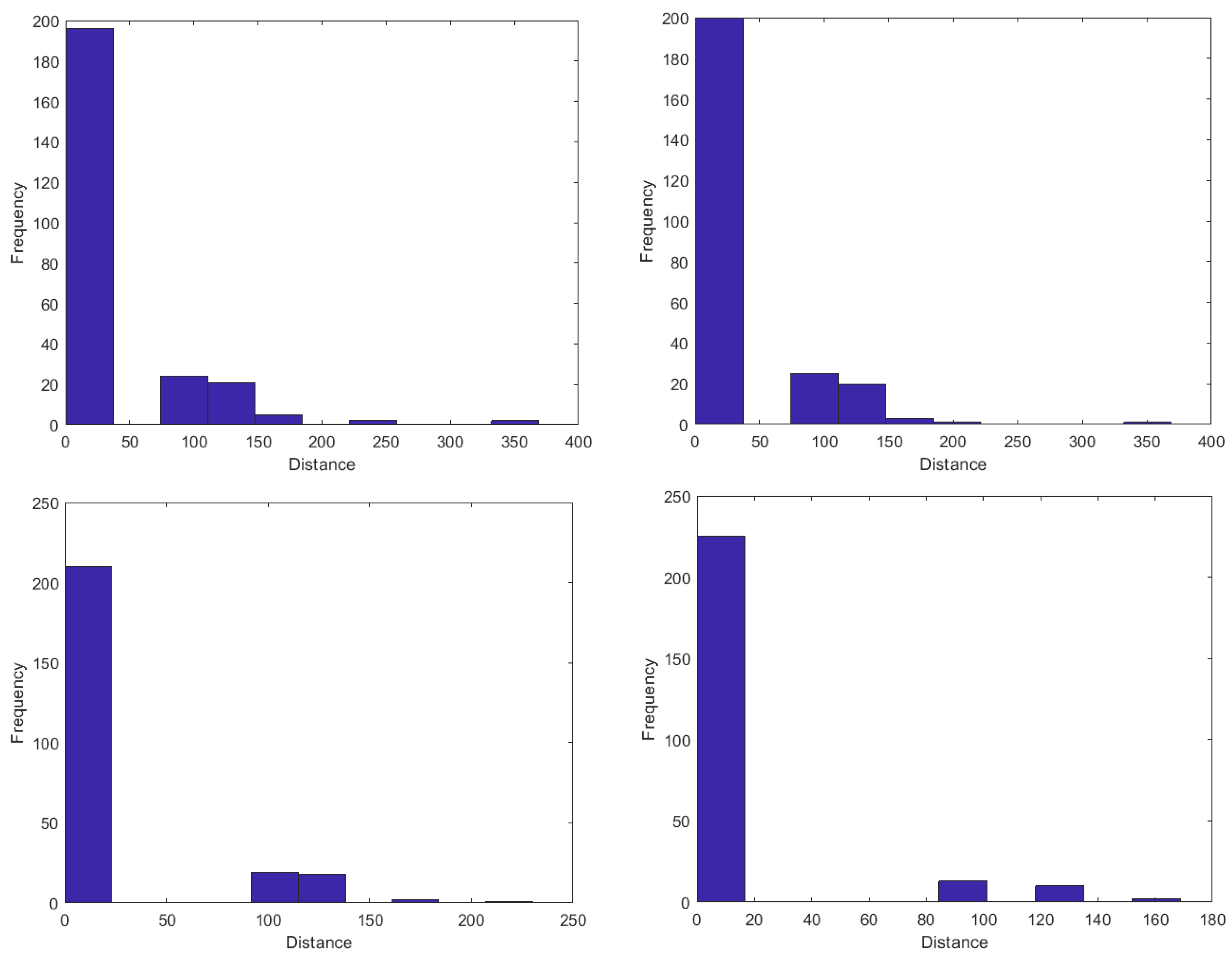
Further experiments were run in order to gauge the performance of the algorithm over a range of piecewise constant jump magnitudes and outlier magnitudes. Two hundred fifty signals were randomly generated in each case with minimum jump and spike magnitudes of to . In each case, the index sets of jump location and outlier location were compared with those used to generate the data using the k-nearest neighbour distance. Histograms of the k-nearest neighbour distance are shown in Figure 5 for piecewise constant detection and in Figure 6 for outlier detection. A larger distance indicates that the outlier and jump locations detected are further away from those used to generate the data. For both jump locations and outlier locations, the distribution of distance shifts left (towards smaller values of distance) as the minimum jump or outlier magnitude increases from to . In general, outliers are detected quite well using the time series decomposition algorithm as the modal bin of the histogram corresponds to very small distances (no distance in most cases).
3.4.2. Real Data
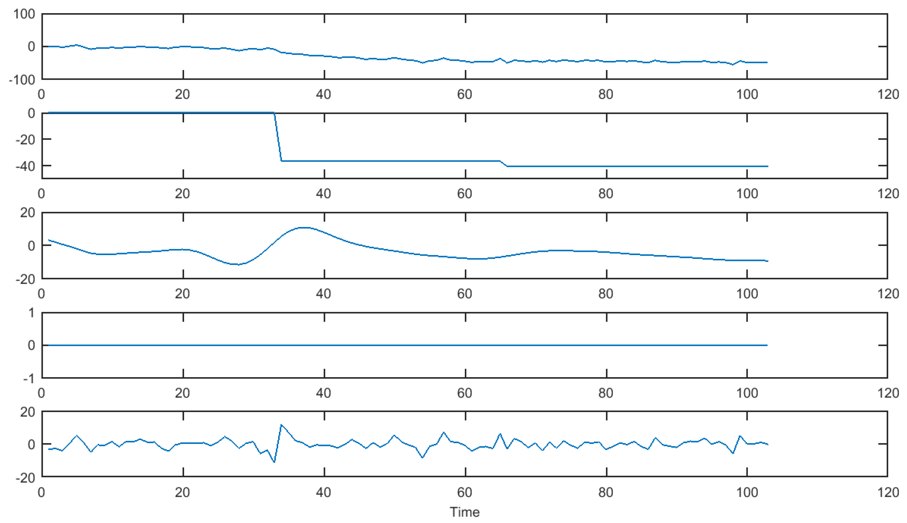
The algorithm has also been used to study time series data relating to ground movement. The data in the first block of Figure 7 seems to have a decreasing trend which is captured by the piecewise affine component in Block 2. The algorithm does not detect any outliers in the data as reflected in Block 4. Seasonal variation is displayed in Block 3. The algorithm seems to converge after as few as 25 iterations.
Author Contributions
E.B. developed applications for data services and supervised the project, S.C. devised the general approach presented in the paper; S.C. and K.J. performed the experiments; S.C., K.J., and B.A.-S. wrote the paper.
Funding
“This research received no external funding”.
Acknowledgments
The work of S.C. is supported by an Innovate UK co-funded research project called Collaborative and AdaPtive Integrated Transport Across Land and Sea (CAPITALS), under TSB grant reference number 102618 awarded under the Integrated Transport: Enabling the End to End Journey competition. Innovate UK is the operating name of the Technology Strategy Board (TSB), the UK’s innovation agency.
Conflicts of Interest
The authors declare no conflict of interest. The founding sponsors had no role in the design of the study; in the collection, analyses, or interpretation of data; in the writing of the manuscript, and in the decision to publish the results.
References
- Box, G.E.; Jenkins, G.M.; Reinsel, G.C.; Ljung, G.M. Time Series Analysis: Forecasting and Control; John Wiley & Sons: Hoboken, NJ, USA, 2015. [Google Scholar]
- Chatfield, C. The Analysis of Time Series: An Introduction; CRC Press: Boca Raton, FL, USA, 2013. [Google Scholar]
- Shumway, R.H.; Stoffer, D.S. Time Series Analysis and It’s Applications; Springer: Berlin, Germany, 2000. [Google Scholar]
- Bianchi, M.; Boyle, M.; Hollingsworth, D. A comparison of methods for trend estimation. Appl. Econ. Lett. 1999, 6, 103–109. [Google Scholar] [CrossRef]
- Young, P.C. Time-variable parameter and trend estimation in non-stationary economic time series. J. Forecast. 1994, 13, 179–210. [Google Scholar] [CrossRef]
- Greenland, S.; Longnecker, M.P. Methods for trend estimation from summarized dose-response data, with applications to meta-analysis. Am. J. Epidemiol. 1992, 135, 1301–1309. [Google Scholar] [CrossRef] [PubMed]
- Visser, H.; Molenaar, J. Trend estimation and regression analysis in climatological time series: An application of structural time series models and the Kalman filter. J. Clim. 1995, 8, 969–979. [Google Scholar] [CrossRef]
- Isermann, R.; Balle, P. Trends in the application of model-based fault detection and diagnosis of technical processes. Control Eng. Pract. 1997, 5, 709–719. [Google Scholar] [CrossRef]
- Hogarth, R.M.; Makridakis, S. Forecasting and planning: An evaluation. Manag. Sci. 1981, 27, 115–138. [Google Scholar] [CrossRef]
- Faraway, J.; Chatfield, C. Time series forecasting with neural networks: A comparative study using the airline data. Appl. Stat. 1998, 47, 231–250. [Google Scholar] [CrossRef]
- Kim, S.J.; Koh, K.; Boyd, S.; Gorinevsky, D. ℓ1 Trend Filtering. SIAM Rev. 2009, 51, 339–360. [Google Scholar] [CrossRef]
- Candès, E.J.; Li, X.; Ma, Y.; Wright, J. Robust principal component analysis? J. ACM (JACM) 2011, 58, 11. [Google Scholar] [CrossRef]
- Mattingley, J.; Boyd, S. Real-time convex optimization in signal processing. Signal Process. Mag. IEEE 2010, 27, 50–61. [Google Scholar] [CrossRef]
- Alexandrov, T.; Bianconcini, S.; Dagum, E.B.; Maass, P.; McElroy, T.S. A review of some modern approaches to the problem of trend extraction. Econ. Rev. 2012, 31, 593–624. [Google Scholar] [CrossRef]
- Brockwell, P.J.; Davis, R.A. Time Series: Theory and Methods; Springer Science & Business Media: Berlin/Heidelberg, Germany, 2013. [Google Scholar]
- Cleveland, R.B.; Cleveland, W.S.; McRae, J.E.; Terpenning, I. STL: A seasonal-trend decomposition procedure based on loess. J. Off. Stat. 1990, 6, 3–73. [Google Scholar]
- Harvey, A.; Trimbur, T. Trend estimation and the Hodrick-Prescott filter. J. Jpn. Stat. Soc. 2008, 38, 41–49. [Google Scholar] [CrossRef]
- Percival, D.B.; Walden, A.T. Wavelet Methods for Time Series Analysis; Cambridge University Press: Cambridge, UK, 2006; Volume 4. [Google Scholar]
- Tibshirani, R.J. Adaptive piecewise polynomial estimation via trend filtering. Ann. Stat. 2014, 42, 285–323. [Google Scholar] [CrossRef]
- Neto, D.; Sardy, S.; Tseng, P. l1-Penalized Likelihood Smoothing and Segmentation of Volatility Processes Allowing for Abrupt Changes. J. Comput. Graph. Stat. 2012, 21, 217–233. [Google Scholar] [CrossRef]
- Levy-leduc, C.; Harchaoui, Z. Catching change-points with LASSO. Adv. Neural Inf. Process. Syst. 2008, 20, 161–168. [Google Scholar]
- Harchaoui, Z.; Lévy-Leduc, C. Multiple change-point estimation with a total variation penalty. J. Am. Stat. Assoc. 2010, 105, 1480–1493. [Google Scholar] [CrossRef]
- Chatfield, C.; Prothero, D. Box-Jenkins seasonal forecasting: Problems in a case-study. J. R. Stat. Soc. Ser. A (Gen.) 1973, 136, 295–336. [Google Scholar] [CrossRef]
- Franses, P.H. Recent advances in modelling seasonality. J. Econ. Surv. 1996, 10, 299–345. [Google Scholar] [CrossRef]
- Osborn, D.R.; Smith, J.P. The performance of periodic autoregressive models in forecasting seasonal UK consumption. J. Bus. Econ. Stat. 1989, 7, 117–127. [Google Scholar]
- McCall, K.; Jeraj, R. Dual-component model of respiratory motion based on the periodic autoregressive moving average (periodic ARMA) method. Phys. Med. Biol. 2007, 52, 3455. [Google Scholar] [CrossRef] [PubMed]
- Tesfaye, Y.G.; Meerschaert, M.M.; Anderson, P.L. Identification of periodic autoregressive moving average models and their application to the modeling of river flows. Water Resour. Res. 2006, 42. [Google Scholar] [CrossRef] [Green Version]
- Weiss, L.; McDonough, R. Prony’s method, Z-transforms, and Padé approximation. Siam Rev. 1963, 5, 145–149. [Google Scholar] [CrossRef]
- Scharf, L.L. Statistical Signal Processing; Addison-Wesley: Reading, MA, USA, 1991; Volume 98. [Google Scholar]
- Tufts, D.W.; Fiore, P.D. Simple, effective estimation of frequency based on Prony’s method. In Proceedings of the 1996 IEEE International Conference on Acoustics, Speech, and Signal Processing Conference, Atlanta, GA, USA, 9 May 1996; Volume 5, pp. 2801–2804. [Google Scholar]
- Van Blaricum, M.; Mittra, R. Problems and solutions associated with Prony’s method for processing transient data. IEEE Trans. Electromagn. Compat. 1978, 1, 174–182. [Google Scholar] [CrossRef]
- Hurst, M.P.; Mittra, R. Scattering center analysis via Prony’s method. IEEE Trans. Antennas Propag. 1987, 35, 986–988. [Google Scholar] [CrossRef]
- Wear, K.A. Decomposition of two-component ultrasound pulses in cancellous bone using modified least squares Prony method–Phantom experiment and simulation. Ultrasound Med. Biol. 2010, 36, 276–287. [Google Scholar] [CrossRef] [PubMed]
- Cadzow, J.A. Signal enhancement—A composite property mapping algorithm. IEEE Trans. Acoust. Speech Signal Process. 1988, 36, 49–62. [Google Scholar] [CrossRef]
- Rukhin, A.L. Analysis of time series structure SSA and Related techniques. Technometrics 2002, 44, 290–290. [Google Scholar] [CrossRef]
- Candès, E.J. Mathematics of sparsity (and a few other things). In Proceedings of the International Congress of Mathematicians, Seoul, Korea, 13–21 August 2014; Volume 123. [Google Scholar]
- Al Sarray, B.; Chrétien, S.; Clarkson, P.; Cottez, G. Enhancing Prony’s method by nuclear norm penalization and extension to missing data. Signal Image Video Process. 2017, 11, 1089–1096. [Google Scholar] [CrossRef]
- Tibshirani, R. Regression shrinkage and selection via the lasso. J. R. Stat. Soc. Ser. B (Methodol.) 1996, 58, 267–288. [Google Scholar]
- Candès, E.J.; Plan, Y. Near-ideal model selection by ℓ1 minimization. Ann. Stat. 2009, 37, 2145–2177. [Google Scholar] [CrossRef]
- Giraud, C. Introduction to High-Dimensional Statistics; CRC Press: Boca Raton, FL, USA, 2014; Volume 138. [Google Scholar]
- Bühlmann, P.; Van De Geer, S. Statistics for High-Dimensional Data: Methods, Theory and Applications; Springer Science & Business Media: Berlin/Heidelberg, Germany, 2011. [Google Scholar]
- Chrétien, S.; Darses, S. Sparse recovery with unknown variance: A LASSO-type approach. IEEE Trans. Inf. Theory 2014, 60, 3970–3988. [Google Scholar] [CrossRef]
- Belloni, A.; Chernozhukov, V.; Wang, L. Pivotal estimation via square-root lasso in nonparametric regression. Ann. Stat. 2014, 42, 757–788. [Google Scholar] [CrossRef]
- Gandy, S.; Recht, B.; Yamada, I. Tensor completion and low-n-rank tensor recovery via convex optimization. Inverse Probl. 2011, 27, 025010. [Google Scholar] [CrossRef]
- Mu, C.; Huang, B.; Wright, J.; Goldfarb, D. Square deal: Lower bounds and improved relaxations for tensor recovery. In Proceedings of the International Conference on Machine Learning, Beijing, China, 21–26 June 2014; pp. 73–81. [Google Scholar]
- Chrétien, S.; Wei, T. Sensing tensors with Gaussian filters. IEEE Trans. Inf. Theory 2017, 63, 843–852. [Google Scholar] [CrossRef]
- Deledalle, C.A.; Vaiter, S.; Fadili, J.; Peyré, G. Stein Unbiased GrAdient estimator of the Risk (SUGAR) for multiple parameter selection. SIAM J. Imag. Sci. 2014, 7, 2448–2487. [Google Scholar] [CrossRef]
- Chretien, S.; Gibberd, A.; Roy, S. Hedging parameter selection for basis pursuit. arXiv, 2018; arXiv:1805.01870. [Google Scholar]
- Fazel, M.; Pong, T.K.; Sun, D.; Tseng, P. Hankel matrix rank minimization with applications to system identification and realization. SIAM J. Matrix Anal. Appl. 2013, 34, 946–977. [Google Scholar] [CrossRef]
- Parikh, N.; Boyd, S. Proximal algorithms. Found. Trends® Optim. 2014, 1, 127–239. [Google Scholar] [CrossRef]
- Nishihara, R.; Lessard, L.; Recht, B.; Packard, A.; Jordan, M. A General Analysis of the Convergence of ADMM. In Proceedings of the International Conference on Machine Learning, Lille, France, 6–11 July 2015; pp. 343–352. [Google Scholar]
Figure 1.
Decomposition of a signal with two outliers.

Figure 2.
Decomposition of a signal with three outliers.

Figure 3.
Decomposition of a signal with five outliers.

Figure 4.
Decomposition of a signal with four piecewise constant jumps.

Figure 5.
Histogram of distance measured for a minimum piecewise constant jump magnitude of (top left), (top right), (bottom left), and (bottom right).
Figure 5.
Histogram of distance measured for a minimum piecewise constant jump magnitude of (top left), (top right), (bottom left), and (bottom right).

Figure 6.
Histogram of distance measured for a minimum outlier magnitude of (top left), (top right), (bottom left), and (bottom right).
Figure 6.
Histogram of distance measured for a minimum outlier magnitude of (top left), (top right), (bottom left), and (bottom right).

Figure 7.
Decomposition of a signal relating to ground movement.

© 2018 by the authors. Licensee MDPI, Basel, Switzerland. This article is an open access article distributed under the terms and conditions of the Creative Commons Attribution (CC BY) license (http://creativecommons.org/licenses/by/4.0/).
Share and Cite
MDPI and ACS Style
Barton, E.; Al-Sarray, B.; Chrétien, S.; Jagan, K. Decomposition of Dynamical Signals into Jumps, Oscillatory Patterns, and Possible Outliers. Mathematics 2018, 6, 124. https://doi.org/10.3390/math6070124
AMA Style
Barton E, Al-Sarray B, Chrétien S, Jagan K. Decomposition of Dynamical Signals into Jumps, Oscillatory Patterns, and Possible Outliers. Mathematics. 2018; 6(7):124. https://doi.org/10.3390/math6070124
Chicago/Turabian StyleBarton, Elena, Basad Al-Sarray, Stéphane Chrétien, and Kavya Jagan. 2018. "Decomposition of Dynamical Signals into Jumps, Oscillatory Patterns, and Possible Outliers" Mathematics 6, no. 7: 124. https://doi.org/10.3390/math6070124
Note that from the first issue of 2016, this journal uses article numbers instead of page numbers. See further details here.