The Relation between the Probability of Collision-Free Broadcast Transmission in a Wireless Network and the Stirling Number of the Second Kind

Abstract

The broadcast performance of the 802.11 wireless protocol depends on several factors. One of the important factor is the number of nodes simultaneously contending for the shared channel. The Medium Access Control (MAC) technique of 802.11 is called the Distributed Coordination Function (DCF). DCF is a Carrier Sense Multiple Access with Collision Avoidance (CSMA/CA) scheme with binary slotted exponential backoff. A collision is the result of two or more stations transmitting simultaneously. Given the simplicity of the DCF scheme, it was adapted for Dedicated Short Range Communication (DSRC) based vehicular communication. A broadcast mechanism is used to disseminate emergency and safety related messages in a vehicular network. Emergency and safety related messages have a strict end-to-end latency of 100 ms and a Packet Delivery Ratio (PDR) of 90% and above. The PDR can be evaluated through the packet loss probability. The packet loss probability $P_L$ is given by, $P_L$ = 1 − ($1-P_e$)($1-P_C$), where $P_e$ is the probability of channel error and $P_C$ is the probability of collision. $P_e$ depends on several environmental and operating factors and thus cannot be improved. The only way to reduce $P_L$ is by reducing $P_C$. Currently, expensive radio hardware are used to measure $P_L$. Several adaptive algorithms are available to reduce $P_C$. In this paper, we establish a closed relation between $P_C$ and the Stirling number of the second kind. Simulation results are presented and compared with the analytical model for accuracy. Our simulation results show an accuracy of 99.9% compared with the analytical model. Even on a smaller sample size, our simulation results show an accuracy of 95% and above. Based on our analytical model, vehicles can precisely estimate these real-time requirements with the least expensive hardware available. Also, once the distribution of $P_C$ and $P_L$ are known, one can precisely determine the distribution of $P_e$.

1. Introduction

A Vehicular Ad hoc Network (VANET) is a special type of Mobile Ad Hoc Network (MANET), where the mobile hosts are the vehicles in the road. They communicate with each other wirelessly to establish a network. A MANET consists of a collection of autonomous mobile nodes that may communicate with each other in a peer-to-peer fashion. No base stations are supported in a MANET environment. Nodes that are in the same radio range of each other can communicate in a single hop fashion. Nodes that are not in the single-hop range can still communicate through the help of intermediate nodes. MANETs are used in situations, such as on a battle field or in major disaster areas, where providing communication infrastructure facility within a short time frame is impossible.

Reduction of road accidents and traffic congestion are two major challenges in today’s society. Although, technologies such as airbags, seat belts and anti-skid brakes are available, the deaths due to road accidents have not come down. At this moment, road traffic fatalities are the eight largest cause of death globally, and they are the leading cause of death among young people aged between 15 and 29 [1]. If no action is taken to address the current crisis, global road traffic fatalities are forecast to rise to more than 2.4 million deaths per annum by 2030 [2].

Dedicated Short Range Communication (DSRC) refers to the use of Vehicle-to-Vehicle (V2V) and Vehicle-to-Infrastructure (V2I) communication that was designed to improve road safety and transportation efficiency. DSRC supports several applications. Among them, Cooperative Collision Avoidance (CCA) is the most important one. In DSRC, V2V communications are established through the use of VANET. VANETs use on-road vehicles as nodes to create an ad hoc network. DSRC supported applications can be classified into three major classes, namely, Safety-related applications, Non-safety-related applications and Infotainment. Speed management and Cooperative navigation are two examples of non-safety applications, while Tourist and Traveller Information Support and Streaming music are two examples of Infotainment. These two classes of applications require communication infrastructure such as a Roadside Unit. The motivation for allowing non-safety applications over DSRC is to create commercial opportunities, thereby, making the DSRC technology more cost-effective.

V2V safety applications are implemented through the VANET environment. In order to reduce the number of fatalities and serious injuries, expensive sensors, radars, cameras and other state-of-art technologies are currently integrated into vehicles. These devices communicate with neighbouring vehicles in an ad hoc fashion when it detects an abnormal situation, such as an accident, slippery road conditions or any other noticeable hazard.

For non-safety applications to coexist with safety applications in the DSRC spectrum, it is absolutely essential to have a mechanism in protecting the safety communication from the interference of non-safety data transmission. Thus, the DSRC standard divided the entire 75 MHz spectrum into seven 10 MHz channels, out of which, one channel called the Control Channel (CCH) is exclusively used for the safety and emergency related communication.

A four-way handshake, namely Request to Send (RTS), Clear to Send (CTS), Data, and Acknowledgement (ACK), is used to transmit a unicast frame. Also, in the absence of an ACK, the size of the Contention Window (CNWD) increases to reduce the probability of successive collisions. However, according to the standard, the handshake mechanism cannot be used for broadcast frames due to the one-to-many nature of the broadcast traffic. Consequently, there is no means for the transmitting node to know whether the packet has been received successfully by all its neighbouring nodes, thus, there are no retransmissions. Furthermore, in the absence of any retransmission, the CNWD size is always kept constant at its minimum value.

V2V communication has a very strict real-time requirement of 100 ms latency from source host’s application-layer to destination host’s application-layer, and a Packet Delivery Ratio (PDR) of at least 90% [3]. Most of the safety messages in a vehicular network are applicable to a region (or a smaller neighbourhood, such as an accident zone), rather than to another individual vehicle. Thus, broadcasting is the most efficient way of disseminating emergency messages. Since the traditional WiFi-MAC protocol (CSMA/CA) satisfied most of the requirements for a V2V communication, it was then chosen as the defacto protocol for vehicular communication. As emergency messages are broadcasted, the contention window is always kept at minimum. Since, there is no MAC layer acknowledgement, the reliability and the system throughput of the broadcast messages can be very low, especially under saturated conditions.

For emergency and safety-related messages in a vehicular network, maintaining a PDR of at least 90% is the most critical aspect. In the absence of any excessive channel noise, maintaining the minimum PDR purely depends on how many vehicles contend for the shared wireless channel concurrently. Collision is certain if two or more vehicles transmit at the same time. In the event of a collision, no data may be recovered, and the entire frame is discarded. The performance of a VANET system is measured based on the wireless channel quality. The PDR is also proportional to this channel quality. In Section 3, we discuss the channel quality in relation to this paper. This section will also outline the motivation for this research work.

The main contribution in this paper are as follows:

• We establish a closed-relation between the number of simultaneously contending nodes and the packet collision probability mathematically through the Stirling number of Second kind. Packet collision probability is then used to evaluate the channel quality. Our results are not only applicable to VANETs, but also to 802.11x wireless protocols in general. Currently, expensive hardware (or a side-channel, or both) is used on every vehicle to measure the channel quality. Using our results, channel quality can be estimated with the least expensive hardware available.
• In the same vein as other research papers available in the literature, we also simulated the VANET environment to obtain the results. The simulated results are compared with the mathematical results for relative-error analysis. Our simulation results show an accuracy of 99.9% compared with the analytical model. Even on a smaller sample size, our simulation results show an accuracy of 95% and above.
• We compared our analytical results with the Markov model proposed by Bianchi [4]. The Markovian model exhibits an error margin of up to 10%. For a smaller contention window size, error margin is less and it increases as the contention window size increases. Also, the marginal error follows a normal distribution curve, for the number of nodes between 1 and CNWD.

The rest of the paper is organized as follows. In Section 2, we provide a brief description of the 802.11 Distributed Coordination Function (DCF) to make this paper self-contained. Section 3 outlines the relation between the PDR and the channel quality in a wireless environment. In Section 4, we establish the mathematical relation. Section 5 deals with simulation and comparison of the results from the mathematical relation. In Section 6, we compare the results obtained through our analytical model with the pioneering work of Bianchi [4]. In Section 7, we present the conclusion and future direction.

Since the collision probability $P_C$ and PDR are inversely proportional, we may use them interchangeably in this paper.

2. The 802.11 $\mathit{DCF}$ Overview

In VANET, deploying a MAC scheme that does not rely on a centralized controller is important due to rapid changes in the network topology. The Carrier Sense Multiple Access (CSMA) protocol originally designed for the wireless network was adapted for vehicular communication. The DCF of the CSMA protocol is the best suitable candidate for vehicular communication due to its decentralized operation, adaptation to various traffic loads, dynamic reconfiguration, and its support for both unicast and broadcast communication.

In DCF, whenever a frame arrives at the MAC layer for transmission, the status of the channel must be checked through the physical carrier sensing. If the channel is currently idle and continues to be idle for one Distributed Inter-frame spacing (DIFS), the station transmits the frame immediately. On the other hand, if the channel is busy at the start, or during one-DIFS wait period, the transmission will not occur immediately, and the backoff algorithm is invoked.

The purpose of the backoff algorithm is to reduce the probability of colliding with any other waiting station when the shared wireless medium becomes idle again. The backoff algorithm works in a slotted time mode. A station performing the backoff process will wait until its backoff counter (BC) is 0 and transmits immediately. The BC value is chosen randomly from a discrete uniform distribution over the interval [0, CNWD-1], where CNWD is the contention window size for the network. The BC can only start to be decremented after an idle DIFS interval. The backoff procedure will decrement its BC value by 1 if no medium activity is indicated for the duration of a SlotTime, and will freeze the process if the medium becomes busy before reaching 0. After freezing the procedure, the medium has to be idle for the duration of a DIFS period before the backoff procedure is allowed to resume. The value of BC is decremented until it reaches zero. As soon as the BC reaches zero, the frame is transmitted provided that the channel is still idle. For a detailed description, please refer to [5].

3. Estimation of Channel Quality in VANETs

The quality of a shared wireless channel that is measured through PDR is affected by two important factors: the channel noise and the number of simultaneously contending nodes. Losses in a Wireless network can be classified into two types: packet collisions, which are due to unfavourable traffic conditions and channel errors, which are due to unfavourable channel conditions [6]. As noted by [6], a collision occurs when a node’s packet overlaps in time with that of another node, which is close enough to the destination to interfere. A channel error occurs when the Signal-to-Noise Ratio (SNR) of the received packet is low due to a large path loss, a deep multipath fade or a white noise. According to them, the total packet loss probability $P_L$ can be expressed as $P_L$ = $1-(1-P_C$)($1-P_e$), where, $P_C$ is the packet collision probability and $P_e$ is the probability of channel error.

The channel error depends on various environmental and operating factors. Thus, it may not be possible to improve them. The only way to improve $P_L$ is by reducing $P_C$.

In [7], $P_C$ estimation is done for an infrastructure-based network. In an infrastructure-based network, nodes obtain spatial information about network traffic via periodically broadcast information from the Access Point (AP), and use it to estimate the probability of collisions. However, in a distributed MANET and VANET environment, the same technique or its modification cannot be used due to the absence of an AP.

Since, it is difficult to estimate $P_e$ in a distributed environment, several authors proposed schemes that estimate $P_L$ based on PDR. PDR can be estimated through mathematical and stochastic models, cooperation between reference nodes, periodic beaconing of nodes or through physical layer radios measuring the radio quality.

In our earlier paper [8], we estimated the node density using the received signal strength without any reference nodes. In that paper, we presented a realistic radio model for the VANET environment. Based on the proposed radio model, we estimated the node density. It may then be used to estimate the PDR indirectly.

Schemes that rely on physical layer mechanisms need to use dedicated receivers to measure the radio quality in order to estimate PDR.

Stochastic and mathematical modelling is another popular way of evaluating the performance of a wireless channel under various operating conditions. Bianchi [4] initiated this study and it has been followed by several others. We review them in Section 6.

Most recently, Cristhian et al. [9] proposed a novel scheme called the Adaptive Distributed Dissemination (ADD) protocol for data dissemination in a VANET environment. To achieve this objective, ADD employs a decentralized stochastic solution for the broadcast data dissemination problem through two game-theoretical mechanisms. The outline of their scheme [9] is as follows: the strategy of the players is to select a forwarding probability that maximizes their payoff using a utility function. The utility function is designed as a function of the player’s availability and the forwarding probability of other players. The availability of a player is a normalized factor based on metrics such as distance from the source of the flooding packet (e.g., an accident vehicle) and estimated bandwidth of the link formed between the node currently holding the packet and each candidate node within its transmission range. As exchanging vehicle information via beacon messages is important for active safety applications, their proposal includes the adaptive traffic beacon (ATB) protocol [10] to seek an uncongested channel, i.e., to prevent packet loss due to collisions, and to reduce the end-to-end delay of the information transfer. We note that the heart of their scheme is the ATB protocol. Their scheme improves $P_L$ by exploiting the ATB protocol and the game-theoretic model. Their protocol fall under p-persistent CSMA, where a packet is transmitted with a probability p. The probability p is chosen based on the game-theoretic model.

In this paper, we evaluate $P_C$ without any underlying assumptions. Once $P_C$ is evaluated, $P_L$ can be evaluated precisely. Our future work involves combining this work and our previous work [8] to propose an accurate scheme for evaluating $P_L$ without any underlying assumptions. Once the precise value is known, it may further be improved based on the existing adaptive schemes. Improving $P_L$ or reducing $P_C$ through an adaptive scheme is not within the scope of this paper.

In literature, several adaptive mechanisms are used to reduce $P_L$ by other means, namely:

• Adjusting the transmission power
• Adapting the frequency of the beacon transmission
• Adjusting the transmission data rate
• Adjusting the contention window of the backoff mechanism
• Modifying the carrier sense threshold
• Transmit frames with some associated probability (e.g., Cristhian et al. [9])

For more detailed information on this topic, Khomami [11] may be referred.

4. The Probability of Collision-Free Broadcast Transmission

In this section, we establish a relation between the number of nodes contending for the shared wireless channel and the Collision Probability $P_C$ in terms of the Stirling number of the second kind. A Stirling number of the second kind (or a Stirling partition number) is defined as the number of ways to partition a set of n objects into k non-empty subsets and is denoted by $S(n,k)$. Whenever a channel is sensed to be busy, every contending node will choose a random backoff timer between [0, $CNWD$-1]. If two or more nodes happen to choose the least contention value, then they transmit simultaneously (as their contention timer becomes zero at the same time). In this case, the collision of their frame is certain if a receiver is within the radio range of both the transmitters.

Let w be the CNWD size. For 802.11x standards that use orthogonal frequency-division multiplexing (OFDM) at the physical layer, including 802.11p (VANET), the size of CNWD for broadcasting is set to 16 [12]. Let E be the set of all nodes that contend for the medium at a particular instance of time and let $\mid E\mid$ = n. If the channel is sensed to be busy, all contending nodes choose a random slot between 0 and CNWD-1 and start their countdown process before they transmit their frame.

Let $T_i$ be the set of nodes that have chosen $sloti$ for their transmission. It is easy to see that ${\bigcup }_{i=0}^{w-1}{T}_i$ = E, and $T_i\bigcap T_j$= ∅ for every $i\ne j.$ Thus, ${\left\{T_i\right\}}_{i=0}^{w-1}$ is a partition of the set E. However, it can be seen that some $T_i$ may be empty, as none of the contending nodes choose $sloti$. A sufficient condition for this case to happen is that $n<w.$ If $n\ge w,$ and we do not allow empty sets in a partition, then the number of different ways of partitioning E into w parts is given by the Stirling number of second kind $S(n,w)$.

While we compute $S(n,w)$, the order in which the partition occurs is immaterial. However, in the problem under consideration, the slots are ordered and the order in which the partition occurs is important to us. Thus, the number of ways of partitioning E into w ordered set is given by $w!\times S(n,w)$ (subject to the condition that empty sets in a partition are not allowed).

Slot-i is defined as the least-numbered slot, if slot 0 to slot (i-1) are not chosen by any nodes, and Slot-i is chosen by at least one node.

When n nodes contend for a channel, and the least numbered slot is chosen by exactly one node, then the node will have a collision-free transmission. The transmission may be error free, provided that there are no excessive white-noise or hidden terminals.

We now provide the following expression to evaluate the probability of collision-free transmission.

Lemma 1.

Let E be the set of nodes contending for a channel and $w\ge 1$ be the contention window size. Then, the total number of ways to partition E into w sets, allowing zero or more empty partitions, is given by Equation (1).

$$K(n,w)=\sum _{k=1}^s\left(\genfrac{}{}{0pt}{}{w}{k}\right)\times k!\times S(n,k),wheres=min\{w,n\}$$

(1)

Proof. 

Let w be the contention window size and E be the set of n-nodes contending for the channel. We now enumerate all possible partitions of E into w-parts allowing zero or more empty-parts.

Case 1: $n<w$. In this case, at least $w-n$ slots are empty. Now E can be partitioned into exactly k non-empty parts and $(w-k)$ empty parts, where $1\le k\le n$

Choosing k non-empty positions out of w available positions is done in $\left(\genfrac{}{}{0pt}{}{w}{k}\right)$ ways. Partitioning E into exactly k non-empty parts in their specific order is given by $k!\times S(n,k)$. Thus in this case we have Equation (2).

$$K(n,w)=\sum _{k=1}^n\left(\genfrac{}{}{0pt}{}{w}{k}\right)\times k!\times S(n,k)$$

(2)

Case 2: $n\ge w$.

The proof for the case when $n\ge w$ follows similarly. ☐

Lemma 2.

Let E be the set of n-nodes contending for a wireless channel, where the contention window size is w. Then the total number of successful transmissions is given by Equation (3), where $K(n,k)$ is the function defined in Lemma 1.

$$T(n,w)=n\times \sum _{k=1}^{w-1}K(n-1,k)$$

(3)

Proof. 

As explained previously, when the channel is sensed to be busy, each node will choose its contention slot for transmission, which is a random value between 0 and CNWD-1. During this contention slot, transmission will be collision-free provided: $slot0$, $slot1$, ⋯, $slot(k-2)$ is not chosen by any nodes, $slot(k-1)$ is chosen by exactly one node and the remaining slots are chosen by ($n-1$) nodes; where $1\le k\le w-1$.

Let no nodes choose $slot0$, $slot1$, ⋯, $slot(k-2)$ and exactly one node out of n nodes choose slot $(k-1)$. This is done in $\left(\genfrac{}{}{0pt}{}{n}{1}\right)=n$ ways. The remaining ($n-1$) nodes can be partitioned into the remaining ($w-k$) slots allowing zero or more empty slots and is given by $K(n-1,w-k)$. Thus, in this case, the total number of ways is $n\times K(n-1,w-k)$.

Adding all the possible ways, we have Equation (4).

$$T(n,w)=n\times \sum _{k=1}^{w-1}K(n-1,k)$$

(4)

 ☐

From Lemma 1 and Lemma 2, we have the following result.

Theorem 1.

There are n nodes contending for a wireless channel with contention window size w. Then, the probability of collision-free transmission is given by Equation (5).

$$P(n,w)=\frac{T(n,w)}{K(n,w)}$$

(5)

The proof follows from the fact that $T(n,w)$ enumerates all transmissions that are collision free and $K(n,w)$ enumerates all possible transmissions.

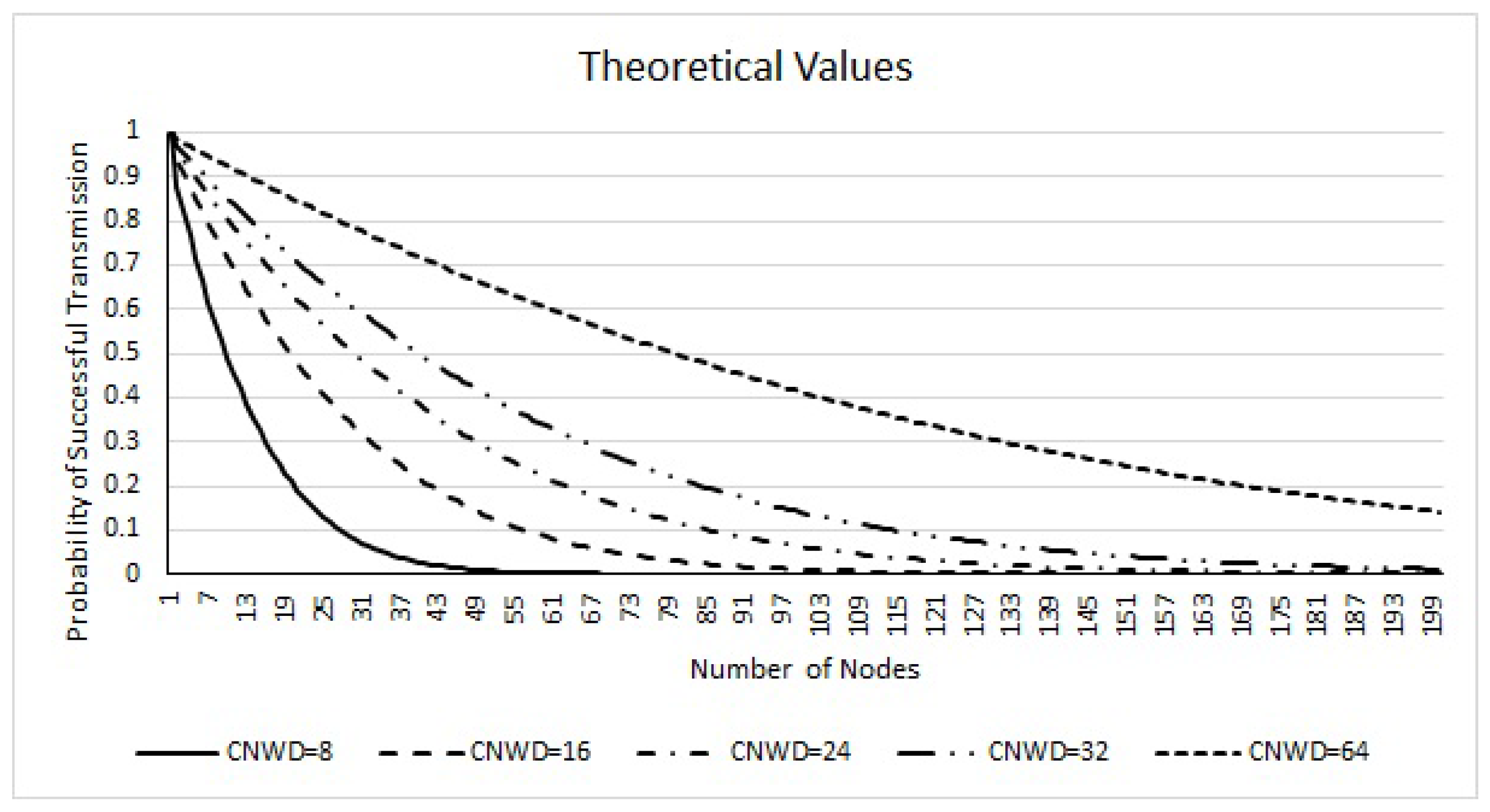
Based on Theorem 1, we compute the probability of collision-free transmission for n-$nodes$ contending for a channel with CNWD = 8, 16, 24, 32, 64 and n ranging from 1 to 200. The results are presented in Figure 1. To achieve a minimum PDR of 90%, we need to have the probability of successful transmission of 0.9 and above. This is obtained when $n<CNWD/4$.

5. Simulation and Comparison of Results

In this section, we present the probability of successful transmission based on the simulation we performed. The results are compared with the theoretical values obtained in Section 4. We have considered 200 vehicles in our simulation. The justification for considering 200 vehicles is as follows:

The reason for choosing 200 as the maximum number of contending vehicles for the channel is related to the maximum number of vehicles within one-hop transmission range of 300 m in a V2V communication. According to the statistics presented in [13], 300 m is the optimum one-hop transmission range for safety applications in V2V communication. In order to calculate the maximum number of vehicles within the transmission range, we consider the size of the vehicles, the spacing between vehicles on the road, the traffic flow theory for highways and urban areas, and the statistics presented in [14,15].

For highway environments, we consider an eight-lane road (four lanes in each direction) and for urban areas, we consider a four-lane street with two lanes in each direction. In highway environments, the maximum number of vehicles varies from 14 to 50 vehicles per lane per km depending on the speed of the vehicles [15]. Therefore, for an eight-lane highway, the maximum number of vehicles within a communication range of 300 m will vary from 34 to 120. Similarly, for an urban environment, we evaluate the maximum number of vehicles in a one-hop transmission range as 72. In order to be on the safer side, for our simulation, we have chosen 200 nodes as a realistic value for the maximum number of vehicles in a one-hop transmission range. However, the “X-axis” may be terminated at the suitable n-value, depending on an urban or a highway environment. We now place these 200 nodes on an eight-lane highway as per [15].

Out of these 200 nodes, n nodes ($1\le n\le 200$) are chosen at random. We then fix the CNWD size. In a single simulated run, these n nodes choose a random backoff timer value between 0 and CNWD-1. If there is exactly one node among the n nodes choose the least backoff value, we call the outcome of our experiment as “success”; otherwise, we termed it as a “failure”. We repeat the same experiment using a different set of n nodes.

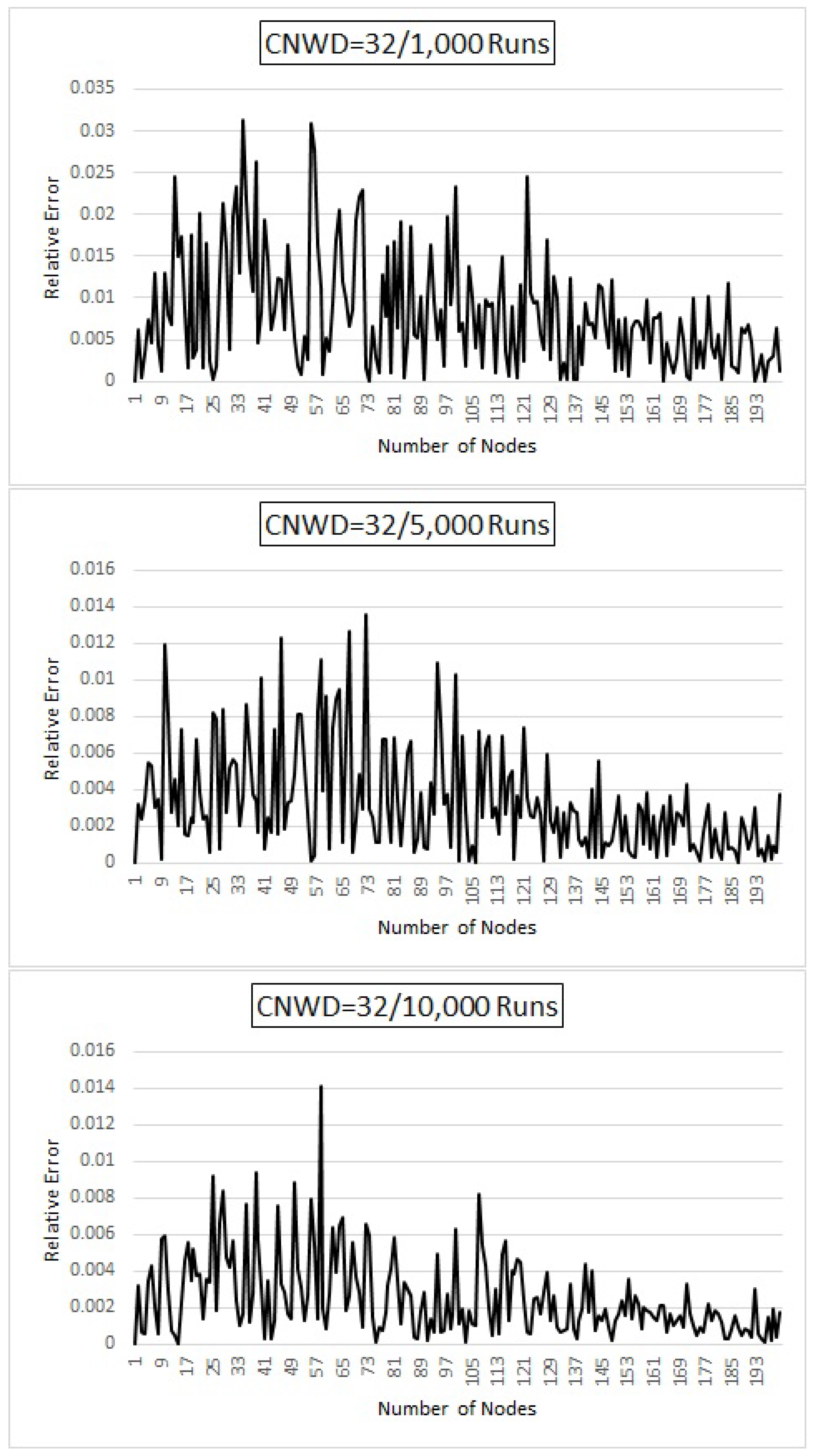
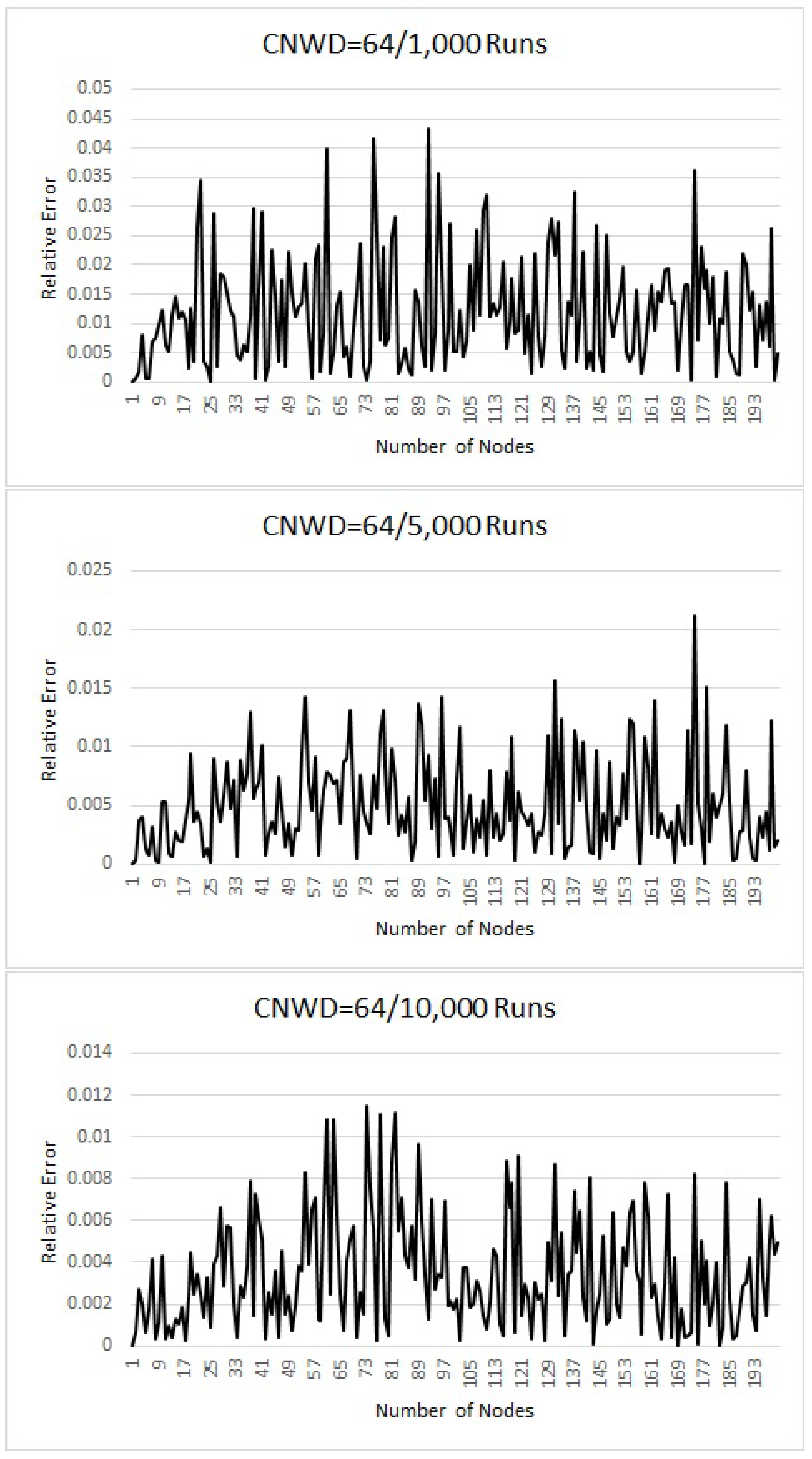
In Probability theory [16], “Stochastic convergence” formalizes the idea that a sequence of essentially random or unpredictable events can sometimes be expected to settle into a pattern. The pattern may for instance be “an increasing preference towards a certain outcome”. Since in our simulation, nodes and the CNWD are selected randomly, it introduces some bias due to random number generators. We then wish to perform the stochastic convergence to analyse our simulator’s asymptotic behaviour. Thus, we ran the experiment 10,000 times. After 1000, 5000 and 10,000 trials, we computed the probability of successful transmission based on the number of “success” obtained against the total number of experiments performed. We do so to analyse our experiment’s performance at intermediate stages towards the convergence. The results are then compared against the theoretical results obtained in Section 4. Since the values are too close, rather than plotting the comparison graphs, we plot the relative-error graph. We define the relative error to be the absolute difference between the theoretical and simulated values. We varied n from 1 to 200 and used different CNWD sizes as per the standard.

We now discuss the results obtained for $CNWD$ = 8, 16, 24, 32 and 64.

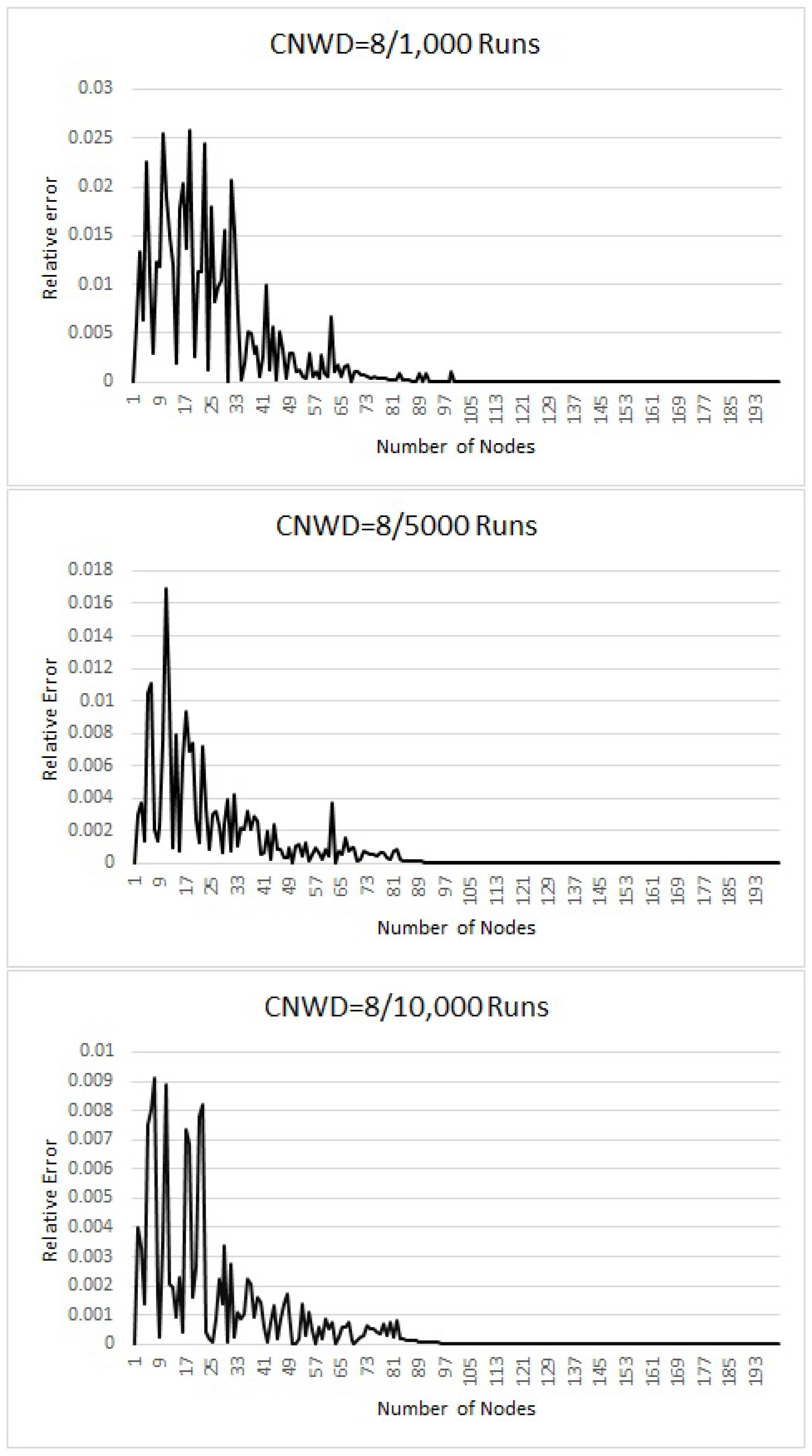
We first discuss the case when $CNWD$ = 8, presented in Figure 2. After 1000 runs, the relative error for n = 0 to 36, it is less than 2.4%. From n = 37 to 45, it is bounded by 0.5% and it then decrease to zero; after 5000 runs, the relative error is less than 1.0% for n = 0 to 15; it is less than 0.5% for n = 16 to 23. It then decreases to zero. After 10,000 runs, the error is less than 1% for n = 0 to 23; between 24 and 59, it is less than 0.3%; it then decreases to zero.

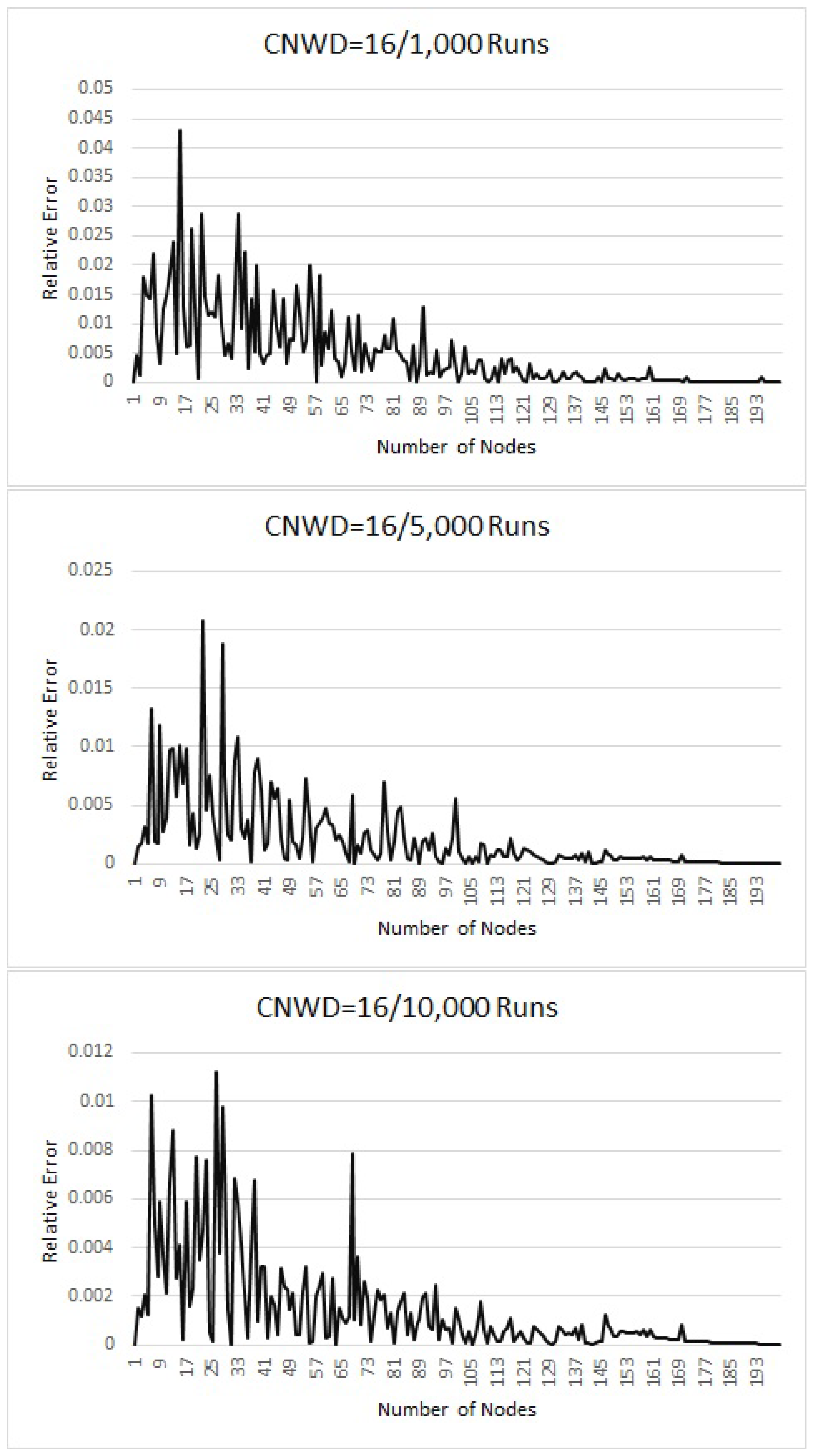
Let $CNWD$ = 16. After 1000 runs, the relative error for n = 0 to 31, it is bounded by 2.4%. From n = 32 to 47, it is bounded by 2.0% and it then decrease to zero; after 5000 runs, the relative error is less than 2.0% for n = 0 to 31; it is less than 1.0% for n = 32 to 47. It then decreases to zero. After 10,000 runs, the error is less than 1.2% for n = 0 to 23; for n between 24 and 59, it is less than 0.8%; it then decreases to zero (refer to Figure 3). This is giving 99.1% accuracy.

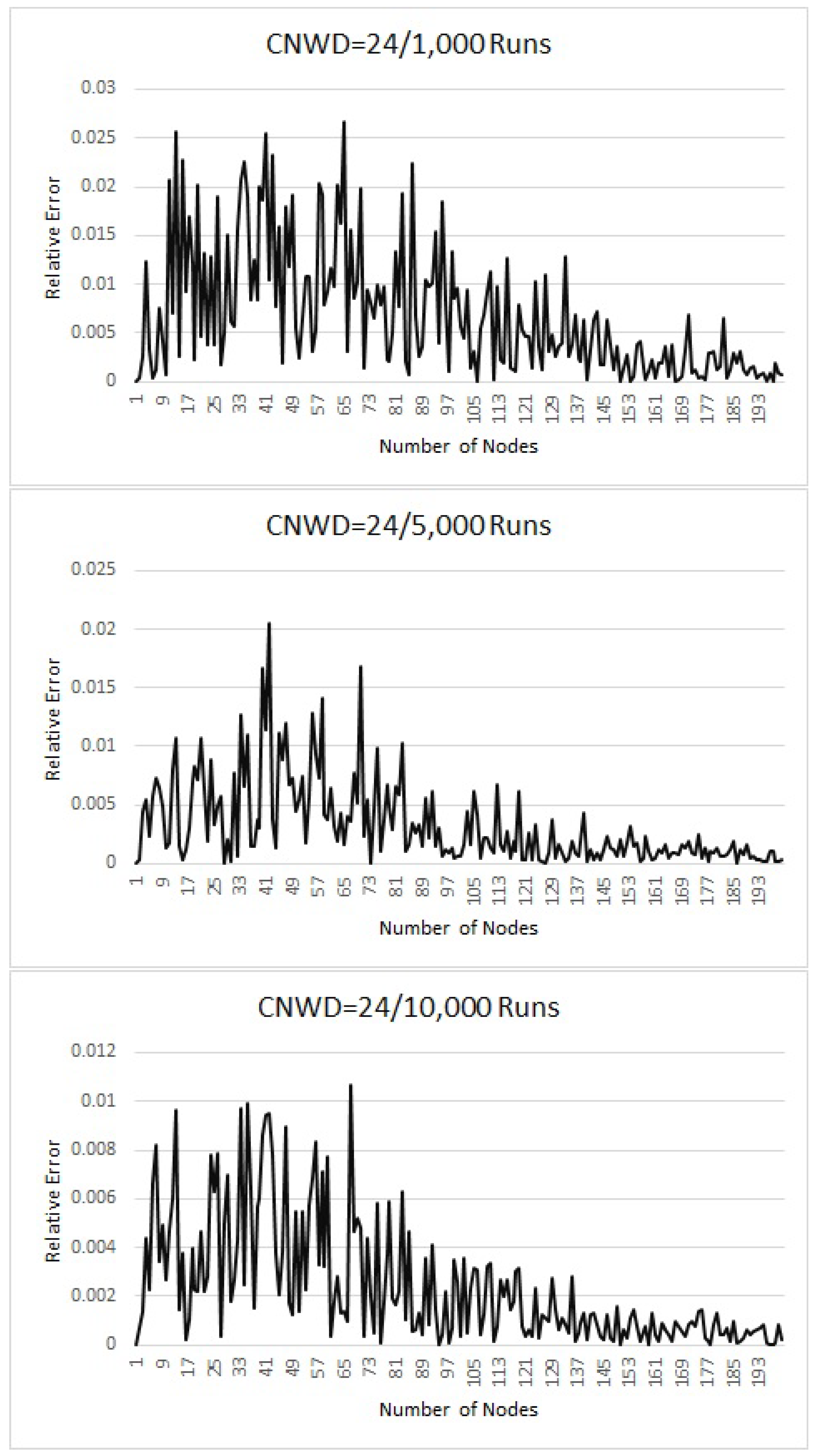
Graphs for $CNWD$ = 24, 32 and 64 (Figure 4, Figure 5 and Figure 6) can be interpreted similarly. As we note from the above results that even for a smaller value of n, and smaller sample size, our simulation results are closer to the theoretical values. It can also be noted from the graphs that for all the possible CNWD considered in this paper, we get an accuracy between 95–99% after 1000 runs.

As we notice from the comparison of our results, presented in Figure 2, Figure 3, Figure 4, Figure 5 and Figure 6 the simulation results are closer to the theoretical values even after 1000 runs. They became much closer after 5000 and 10,000 runs. This proves that our simulation values converge to the theoretical values. While we are performing the simulation, we noticed that the relative error is less than 5% even after 100 runs. Thus, a prediction can be made with 95% confidence even from smaller sample space [16] .

6. Comparison of Our Analytical Model with Biachi’s Model

As we mentioned in Section 3, the packet loss probability $P_L$ = 1 − ($1-P_e$)($1-P_C$). The probability of channel error depends on the environmental and operating conditions. Thus, it is unpredictable. The PDR is inversely proportional to $P_L$. There are numerous research articles available in the literature that reduces $P_L$ through various adaptive transmission strategies. Thus, they obtain their objective of increasing PDR. There only few research articles available in the literature that estimates the collision probability $P_C$. They are based on stochastic process and Markov modelling. Since we estimate $P_C$ through exact probability in this paper, we compare with respect to Markov models in this section.

In the past, numerous authors analysed the performance of 802.11 DCF based on simulation under various operating conditions. In [4], Bianchi initiated a systematic study on the performance of 802.11 DCF under ideal channel conditions (no hidden terminal, external noise and channel capture). His work deals with both RTS/CTS based unicast transmission with exponential backoff algorithm and the broadcast transmission with constant backoff window. His analytical technique uses a Markov chain model to compute the system performance. After this pioneering work, several authors (see for e.g., Ma and Chen [17] and Ziouva and Antonakopoulos [18]) made changes to his model to suit different conditions. However, still today, Bianchi’s work is regarded as a standard in this research field.

His analysis is divided into two distinct parts. First, he studied the behaviour of a single station with the Markov model to obtain the stationary probability $\tau$ that the station transmits a packet in a randomly chosen slot-time. Then, he expressed the throughput and probability of successful transmission based on the computed $\tau$. For a constant backoff window, it was computed that $\tau =\frac{2}{W+1}$, where W is the contention window size. The probability of a successful transmission is given by $P_s$ = $\frac{n\times \tau \times {(1-\tau )}^{(n-1)}}{1-{(1-\tau )}^n}$. Here $P_s$ is given by the probability that exactly one station transmits on the channel, conditioned on the fact that at least one station transmits during that slot.

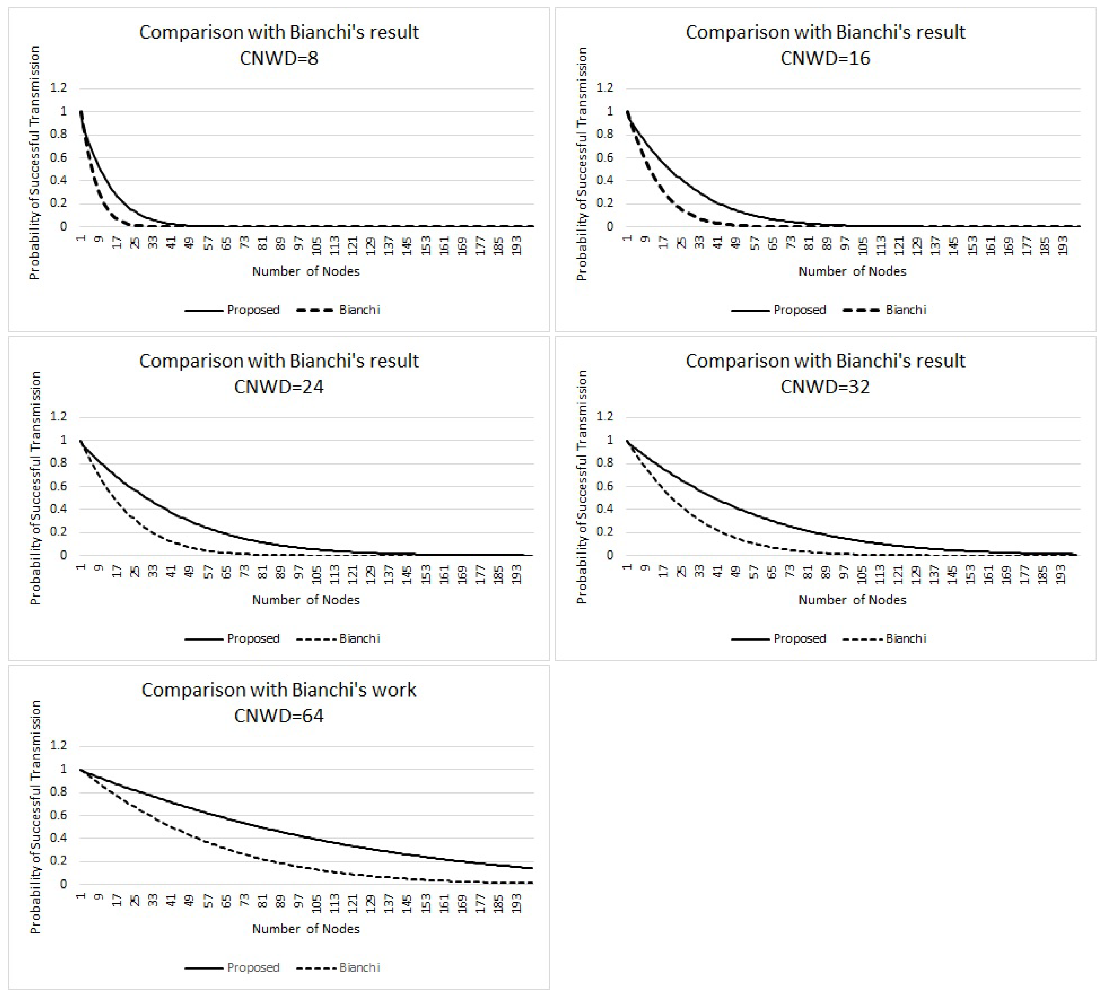
We compared our analytical results with results obtained through Markov model based on Bianchi’s work. Since Markov models obtain stability over time, there is a marginal error between Bianchi’s model and the exact probability. We made the following observation:

• Markov model results in probability of successful transmission (($1-P_C$)), that is less than the exact probability. It exhibits an error margin of up to 10%. For a smaller contention window size like 8, error margin is less and it increases gradually as the contention window size increases to 16, 24, 32 and 64.
• It can be observed from the graphs that if n is small (typically $<CNWD$), Markovian values are closer to the actual probability. It then increases gradually and peaks around $n=2\ast CNWD$ for CNWD 8 and 16 and $1.5\ast CNDW$ for CNWD 24, 32 and 64. It then equals to the exact probability around $n=4\ast CNWD$ for all values of CNWD we simulated.
• It can be seen from the graphs (Figure 7) that marginal error follows a normal distribution curve for the number of nodes between 1 and CNWD. Whenever n is less than $1,5\ast CNWD$, there is more probability that some slots may not be taken by any nodes. If the initial slots are empty, they are counted towards $1-P_s$. Thus, the system has more marginal error for $1\le n\le 1.5\ast CNWD$. Whenever $n>1.5\ast CNWD$, the probability of having an empty slot is close to zero. Thus the Markovian values are close to the exact probability.

In our case, we compute the exact probability of successful transmission based on enumeration. Thus our analytical model produces exact values.

Our comparison results are presented in Figure 7.

The following properties can be observed between the theoretical values and the Markov chain based simulation values obtained by Bianchi.

For $CNWD$ = 8, the difference between the theoretical and Markov chain based simulated values increases from 0 to 0.2 for n = 0 to 15; and then decreases to zero for n = 16 to 40; it is then identical. For $CNWD$ = 16, the difference between the theoretical and Markov chain based simulated values increases from 0 to 0.2 for n = 0 to 23; and then decreases to zero for n = 26 to 79; it is then identical.

In a similar fashion, other graphs can be interpreted.

7. Conclusions and Future Direction

In this paper, we established a relation between the probability of successful transmission (and $P_C$) in a wireless network and the Stirling number of the second kind. Our simulation results are identical to the theoretical values. If we assume that $P_e$ is stable, then based on our results, one can precisely estimate the PDR without any expensive hardware or field-trials. PDR is directly proportional to ($1-P_e$)($1-P_C$). Thus, PDR is affected by the channel noise due to the environment and operating conditions. During vehicular field trials, expensive radio hardware are used to record $P_e$ for a given Suburb or a City. Once $P_e$ and $P_C$ are known , PDR can be evaluated more precisely. Our algorithm can also be used by other existing adaptive algorithm to fine-tune their outcome based our calculated $P_C$. Our future work involves combining the radio model presented in [8] and the results presented in this paper to propose a solution that outputs $P_L$ without any underlying assumptions such as adaptive beaconing.